Infrared Imaging of Capella
with the IOTA Closure Phase Interferometer

Abstract

We present infrared aperture synthesis maps produced with the upgraded IOTA interferometer. Michelson interferograms on the close binary system Capella ($\alpha$ Aur) were obtained in the $H$-band between 2002 November 12 and 16 using the IONIC3 beam combiner. With baselines of $15$ m $\leq B\leq 38$ m, we were able to determine the relative position of the binary components with milliarcsecond (mas) precision and to track their movement along the $\approx 14\arcdeg$ arc covered by our observation run. We briefly describe the algorithms used for visibility and closure phase estimation. Three different Hybrid Mapping and Bispectrum Fitting techniques were implemented within one software framework and used to reconstruct the source brightness distribution. By dividing our data into subsets, the system could be mapped at three epochs, revealing the motion of the stars. The precise position of the binary components was also determined with model fits, which in addition revealed $I_{Aa}/I_{Ab}=1.49\pm 0.10$ and apparent stellar uniform-disk (UD) diameters of $\Theta_{Aa}=8.9\pm 0.6$ mas and $\Theta_{Ab}=5.8\pm 0.8$ mas.

To improve the $u,v$-plane coverage, we compensated this orbital motion by applying a rotation-compensating coordinate transformation. The resulting model-independent map with a beam size of $(5.4\times 2.6)$ mas allows the resolution of the stellar surfaces of the Capella giants themselves.

1 Introduction

Aperture synthesis images, obtained using an interferometer with multiple baselines and closure phases, provide a much more assumption-free way to interpret interferometric data astrophysically than the simple fitting of models to single-baseline fringe amplitudes does. Therefore, imaging capabilities will be of special importance for the upcoming generation of ground-based and space interferometers. In this paper, we present the results of an initial attempt to use the Infrared Optical Telescope Array (IOTA) for imaging in the near infrared. Since this was to be the first effort to construct an image at IOTA, we decided that it was important to observe an object with a well known brightness structure in order to demonstrate the instrument’s capabilities. Therefore, we chose to observe the strongly resolved spectroscopic binary Capella ($\alpha$ Aurigae) so that our maps could be compared to the results of earlier studies.

The first spectroscopic measurements by Campbell (1899) revealed the components Capella Aa and Ab (classified today as G8 III and G1 III (Johnson et al., 2002)). The system also became the first binary to be separated by an optical interferometer (Anderson, 1920). The orbit was determined with high precision in 1994 using the Mark III interferometer by Hummel et al. (1994). In 1996 Baldwin et al. presented the first optical ($\lambda=830$ nm) aperture synthesis map of Capella using the Cambridge Optical Aperture Synthesis Telescope (COAST) with a longest baseline of $B=6.1$m. Two years later Young used the same instrument to map Capella in the near infrared ($\lambda=1.3$ $\mu$m; Young, 1999).

We observed Capella on five nights in November 2002 in the $H$-band ($\lambda=1.65\mu$m; $\Delta\lambda=0.3\mu$m). In this paper, we review the data reduction procedure used to determine visibilities and closure phases from the raw interferometer data, and we present model fits and images derived from the visibility and closure phase data. By investigating the well-studied Capella system, we have been able to calibrate the closure phase sign and to determine the overall behaviour of this recently upgraded 3-telescope interferometer. One of the mapping procedures described within this paper has also been used to generate the maps presented in Monnier et al. (2004) depicting the binary $\lambda$ Virginis.

2 Observations

Table 1: Observation Log

Date [UT]	Start time [UT]	No. exposures	Calibrators
11/12/02	07:43	20	$\alpha$ Cas, $\beta$ Aur
	10:11	27	$\beta$ Aur
	12:00	16	$\beta$ Aur
11/13/02	07:19	26	$\delta$ Aur, $\beta$ Aur
	09:09	20	$\beta$ Aur, $\delta$ Aur
	10:45	24	$\delta$ Aur, $\beta$ Aur
11/14/02	05:51	25	$\kappa$ Per, $\beta$ Aur
	08:24	21	$\delta$ Aur, $\beta$ Aur
	10:25	39	$\delta$ Aur, $\beta$ Aur
	12:06	19	$\beta$ Aur, $\delta$ Aur
11/15/02	07:08	25	$\alpha$ Cas, $\delta$ Aur
	09:28	53	$\delta$ Aur
	11:34	18	$\delta$ Aur
	12:50	6	$\delta$ Aur
11/16/02	09:12	45	$\delta$ Aur, $\beta$ Aur
	12:22	17	$\delta$ Aur

Interferometer Configuration used:
2002 Nov 12-14: A35, B15, C0
2002 Nov 15-16: A15, B15, C0
where A, B, C denotes the individual telescopes and the number of their position
on the north-east (for A and C) or south-east baseline (for B) in meters.

The IOTA was constructed jointly by the Smithsonian Astrophysical Observatory (SAO), Harvard University, the University of Massachusetts (UMass), the University of Wyoming, and MIT/Lincoln Laboratory (Traub et al., 2003). This 3-telescope interferometer located at Fred Whipple Observatory atop Mount Hopkins, Arizona, demonstrated first closure phases on 2002 February 25. IOTA’s telescopes can be moved on an L-shaped track and are mounted on stations $\approx 5$ m and $\approx 7$ m apart. With track lengths of 15 m (south-east direction) and 35 m (north-east direction), baselines up to 38 m can be formed. The collecting optics consist of f/2.5 45 cm Cassegrain primary mirrors, which are fed by siderostats. The atmospherically induced motion of the image is compensated by tip-tilt servo systems mounted behind the telescopes. Passing various mirrors and path-compensating delay lines, the beams are deflected into the laboratory, where the infrared component of the beam is coupled onto the IONIC3 pair-wise beam combiner (Berger et al., 2003). This combines the beams symmetrically with a ratio of 50:50.

For each baseline the beam combination produces two complementary outputs which are simultaneously acquired by a PICNIC-camera (Pedretti et al., 2004). Using piezo scanners installed in two optical path delays, the optical path delay (OPD) can be modulated to scan temporally through the interference fringe pattern.

Each observation on the target object is completed by the acquisition of four calibration files. One of these files measures the camera background signal with the light from all telescopes shuttered out. For the other three files, the light of two telescopes is shuttered out alternately. This allows us to measure the instrument transmission by determining the coefficients of the transfer matrix ($\kappa$ matrix,  Coudé Du Foresto et al., 1997).

The observations presented in this paper were obtained at the IOTA between UT 2002 November 12 and 16. During this time we made observations in two three-telescope configurations in order to obtain a reasonable sampling of the $u,v$ plane for the Capella image. A log of the observations is presented in Table 1.

3 Data Reduction

(see Figure attached)

Figure 1: Representative corrected interferograms, all taken 2002Nov13 on the BC baseline. The selected scans represent typical conditions with low noise ($\alpha$ Cas), high noise ($\delta$ Aur), and interfering resonance ($\alpha$ Lyn). The wavelet spectral density power spectra shown in the lower panels are calculated from the corresponding raw interferograms. On the ordinate of the CWT plots, the scale quantity is given which is equivalent to the period and inversely proportional to the frequency of the corresponding rescaled wavelet. The contours demonstrate how our departitioning algorithm removes regions not connected to the area with the highest peak and separates the fringe peak from the piston and resonances for the visibility estimation.

IOTA produces raw fringes by scanning the optical path delay through the position of the white light fringe in the instrument. The fringes which are observed must then be converted into visibilities and closure phases for imaging and model fitting. We have reduced the raw fringe data in a sequence of steps.

An important first step is to locate the fringes within the raw data scans in order to determine the optical path delay in the IOTA system. If fringes are found, the next step is to calibrate photometric fluctuations due to atmospheric seeing. By using the transfer matrix, the coupling of the stars to the optical inputs of the beam combiner and the internal coupling of the beams within the combiner (Coudé Du Foresto et al., 1997) are taken into accont as well.

In order to form a photometrically calibrated scan, we make use of the fact that for the 3-beam pairwise combination scheme used the photometric information can be obtained for each measurement using linear combinations of the interferometric signals (similar to the procedure used by  Monnier, 2001). This requires a matrix inversion, which might be sensitive to numerical instabilities, especially in the case of low signal-to-noise ($S/N$). For this reason, we smooth the scan by convolving it with a Gaussian before solving for the photometry for each individual pixel. The photometric calibration is performed for the two complementary signals of each baseline separately. Remaining residuals are removed by subtracting the two complementary outputs for each baseline.

The upper panels of Figure 1 illustrate how the data might look for different conditions after these basic data reduction steps.

Each observation at IOTA consists of measurements of hundreds of fringes obtained over a time period of a few minutes. Typically, we have estimated visibilities and closure phases for each individual realization of a fringe and then averaged the results for many fringes to obtain the final result.

3.1 Visibility Estimation

The scans through the white light fringe follow a particular functional form. Assuming a bandwidth filter with idealized rectangular transmission, the instrumental response expected for a point source is given by the product of a sinc-envelope, with width inversely proportional to the bandwidth of the input signal, and a cosine function representing the interference fringes. The amplitude of the fringe envelope reflects the raw visibility. However, this measurement must be calibrated with observations of unresolved reference stars or stars of known diameter in order to remove instrumental and atmospheric effects. Typically, each observation of a target source is bracketed by observations of unresolved stars to provide a calibration of the instrument. In this work, all target observations are enclosed by at least one such calibration measurement on each side of the target observation. The results for the calibration stars are interpolated linearly to calibrate the raw visibilities for the interferometric efficiency of the system, yielding the calibrated target visibility.

During our observation run we noticed a minor technical problem which became a dominating issue for data reduction: the scanning piezo mirrors showed a mechanical resonance (see 3rd panel of Figure 1), resulting in multiple additional peaks within the power spectrum of the acquired scans. The data reduction procedure most commonly used by the interferometry community (e.g. Baldwin et al., 1996) estimates the visibility by integrating over the fringe peak within interferogram power spectra after averaging and background subtraction. To improve the visibility estimation for our resonance-influenced data, we implemented two alternative methods to estimate the visibility amplitude.

Since the interfering resonance only affects the internal structure of the fringes, we implemented a Fringe Envelope Fitting (FEF) algorithm which filters the peaks of the fringe packet. The position of these local minima and maxima is then fitted to the analytic sinc-envelope function with the envelope amplitude, the width, and the position as fitting parameters. For low $S/N$ this algorithm tends to overestimate the fringe amplitude. Analyzing the resulting bias by simulating fringes with additive Gaussian noise, we found a bias on the fitted fringe amplitude which depends exponentially on the noise. Based on these simulations we were able to correct the fitted visibilities down to $S/N\approx 1$.

Motivated by Ségransan et al. (2003), we also implemented a data reduction procedure based on the Continous Wavelet Transform (CWT). In multiscale analysis, the time signal is decomposed into the two-dimensional time-frequency space by measuring the response of a translated and scaled mother-wavelet function to the measured signal. Compared to the Fourier transform (FT), which is based on periodical sinusoidal waves, the use of a localized mother wavelet allows the precise localization of the power within the signal (Torrence and Compo, 1998). For the mother wavelet, we used the Morlet function, which is given by a sinusoidal multiplied with a Gaussian and therefore similar to the analytic fringe function as noted above. The absolute square of the complex wavelet function defines the wavelet spectral density spectrum.

From this density spectrum, we remove all features below a particular significance level (e.g. $35\%$ scaled to the peak). Resonance (see Fig. 1) or an uncompensated change in piston during the fringe scan might result in several non-connected areas. Therefore, we run a filling algorithm which removes all regions which are not connected to the area containing the main signal. The integral over the remaining region is used as an estimate of the fringe power.

The measured width of the remaining region in the OPD and scale domain is then compared to the expected width and used as a selection criteria to reject scans with a high piston. Even for good scans, the CWT is contaminated by additive noise. To determine the level of this noise, we integrate in the CWT along the OPD axis towards both directions, starting $5\mu$m from the border of the fringe region. The extend of this noise region along the scale axis is given by the extend of the fringe peak region. This averaged background noise level is subtracted from the fringe power. Noticing that the CWT is a non-linear transformation, we confirmed the proper behavior of our algorithm by performing extensive simulations.

The visibilities obtained with the FEF and CWT algorithm are in good agreement, even if the CWT algorithm seems to be superior for cases with low $S/N$. The accuracy of the measured visibilities is limited primarily by calibration. For error estimation we include, beside the statistical errors for each data set, a calibration error for each night which was estimated by the scattering of the calibrator visibilities during that particular night. For good seeing conditions this calibration error $\Delta V_{calib}^{2}$ is typically around $\pm 1\%$ (2002 Nov 12-15), while for worse conditions it may rise to $\pm 2\%$ (2002 Nov 16).

3.2 Closure Phase Estimation

Since we are observing on the three baselines $AB,BC,AC$ simultaneously, the fringe phases $\phi_{AB}$, $\phi_{BC}$, $\phi_{AC}$ can be measured. Simultaneous measurement of three phases in turn allows a new quantity, the closure phase $\Phi$ (CP, Jennison, 1958), to be estimated. The CP has enormous value since it is unaffected by atmospheric propagation effects, and through measurements of CP and visibility amplitudes, it is possible to create aperture synthesis images. In the following we briefly describe our methods for estimating this essential interferometric observable.

The estimation of CP begins with the location of the fringes for each baseline within the raw scans. The phase of each fringe must be determined within the same temporal window within the scan in order to assure that all phases are measured at the same time and within the coherence time of the atmosphere. Thus, we locate the median delay for the centers of the three fringe packets and determine the phase of each baseline within a short window of width $3\mu$m centered on that OPD. The FT of the windowed fringe results in a strong peak at the frequency of the fringe. In the IOTA three-baseline system, the frequencies of these peaks for the three fringes obey a “closure” relationship such that $\nu_{AB}+\nu_{BC}-\nu_{AC}=0$, and if this relationship is not obeyed by the data, then there is a good chance that one or more of the peaks is spurious. For these reasons, we reject scans which do not obey this frequency closure relation. For scans that do pass this test, we may then use the phases of the FT’s for the three fringes to compute the CP: $\Phi=\phi_{AB}+\phi_{BC}-\phi_{AC}$. Unresolved calibrators, for which the CP is known to be zero, are used to define the instrumental CP-offset.

Using the above algorithm, we have estimated closure phases for all of the observations obtained during our run. From the scattering of the calibrator CP over the individual nights we include calibration errors $\Delta\Phi_{calib}$ between $\approx 0.2\arcdeg$ and $1.1\arcdeg$. Under good seeing conditions, the IOTA/IONIC3 instrument is able to measure CP with high precision with systematic errors of the order of $1.0\arcdeg$ or less. As a conservative value we assume $\Delta\Phi_{sys}=2.0\arcdeg$.

3.3 Investigating the Effect of Bandwidth Smearing

After presenting the details of our procedures for visibility and CP estimation, we want to investigate a potential influence of the bandwidth smearing effect on our data.

For extended sources, this effect will reduce the complex degree of coherence at those points of the brightness distribution that are separated in delay from zero optical path delay $\tau$ by amounts comparable to the width of the fringe packet. As a consequence, the detailed instrumental response will be more complicated than the point-source response. Thus, estimation of visibilities and closure phases using the point source response as a template could lead to some systematic errors.

For a rectangular spectral bandpass profile, the complex degree of coherence $c$ is given by

$$c(\tau)=\frac{\sin\left(\pi\tau\Delta\lambda/\lambda^{2}\right)}{\pi\tau\Delta\lambda/\lambda^{2}}.$$ (1)

To estimate the loss of coherence for a particular projected baseline $B_{\bot}$, the coherent field of view $\Delta\alpha=\tau/B_{\bot}$ can be defined as the angular separation for which the fringe of an off-axis point source will be centered right on the first zero point of the fringe envelope of the on-axis point source. In this case, just half of the fringe power from both sources will overlap. Using Equation 1, we obtain $\Delta\alpha=\lambda^{2}/(B_{\bot}\Delta\lambda)\approx 49$ mas for our longest baseline used (AB on the nights of UT2002Nov12-14). The comparison with the separation of the Capella stars ($s\approx 46$ mas) shows that we just reach the limit where bandwidth smearing might play a role.

Since in the regime of marginal bandwidth smearing the contrast decreases with distance from zero OPD in a well-defined way, a correction can be applied. In the given case we correct the visibility $V_{UD}(\Theta)$ of a uniformly bright disk of diameter $\Theta$. Assuming totally coherent combination, $V_{UD}$ can be written as

$$V_{UD}(\Theta)=\frac{2J_{1}(k\Theta B_{\bot})}{k\Theta B_{\bot}},$$ (2)

where $J_{1}$ denotes the Bessel function of first kind and first order.

To determine the delay-affected visibility $V_{UD}^{BW}$, we define

$$V_{UD}^{BW}(\tau)=c(\tau)V_{UD}$$ (3)

In the case of a binary star with two UDs of diameter $\Theta_{Aa}$ and $\Theta_{Ab}$ the resulting interferogram is given by the composition of two fringes with different delays $\tau_{Aa}$ and $\tau_{Ab}$. Since the delay at which the combined fringe is evaluated depends on the brightness ratio of the individual fringes, it is appropriate to evaluate the two correction factors relative to an effective delay $\tau_{\textnormal{eff}}$, given by the center of intensity of the combined fringe packet:

$$\tau_{\textnormal{eff}} = \frac{I_{Aa}\tau_{Aa}+I_{Ab}\tau_{Ab}}{I_{Aa}+I_{Ab}}$$ (4)

$$V_{UD,Aa}^{BW} = c(\tau_{\textnormal{eff}}-\tau_{Aa})V_{UD}(\Theta_{Aa})$$ (5)

$$V_{UD,Ab}^{BW} = c(\tau_{\textnormal{eff}}-\tau_{Ab})V_{UD}(\Theta_{Ab}).$$ (6)

The fact, that our procedure for closure phase estimation does not measure the phases over the whole fringe packet could be of advantage in the regime of marginal bandwidth smearing. As described in chapter 3.2, we measure the phases within a narrow temporal window around the center of the composite fringe where the interferograms overlap properly.

4 Model Fitting

Making use of the expression for the visibility of a delay-affected UD, the complex visibility $\mathbf{V}$ of a close binary system with a position vector $\vec{x}$ can be written as

$$\mathbf{V}(\vec{x})=\frac{I_{Aa}V_{UD,Aa}^{BW}+I_{Ab}V_{UD,Ab}^{BW}e^{-ik\vec{B}\cdot\vec{x}}}{I_{Aa}+I_{Ab}},$$ (7)

with $\vec{B}=(u,v)$ for the baseline vector and the wave number $k=2\pi/\lambda$. In strictly formal notation, an additional overall phase factor appears on the right-hand side of Equation 7. Since this phase factor merely moves the fringe pattern underneath the envelope it neither effects the visibility nor the CP and can be neglected.

We performed least square model fits, equally weighting $N_{V}$ individual visibility and $N_{\Phi}$ CP measurements with

$$\chi^{2} = \chi_{V^{2}}^{2}+\chi_{\Phi}^{2}$$ (8)

$$\chi_{V^{2}}^{2} = \sum\limits_{i=1}^{N_{V}}\left(\frac{V_{i}^{2}-V_{model}^{2}}{\sigma_{V^{2}}}\right)^{2}$$ (9)

$$\chi_{\Phi}^{2} = \sum\limits_{i=1}^{N_{\Phi}}\left(\frac{\Phi_{i}-\Phi_{model}}{\sigma_{\Phi}}\right)^{2},$$ (10)

with the model visibilities $V_{model}$ and closure phases $\Phi_{model}$ calculated from the complex visibility:

$$V_{model}^{2}(u,v) = \left|\mathbf{V}(u,v)\right|^{2}$$ (11)

$$\Phi_{model}(u_{1},\ldots,v_{3}) = \sum_{i=1}^{3}\tan^{-1}\frac{\Im(\mathbf{V}(u_{i},v_{i}))}{\Re(\mathbf{V}(u_{i},v_{i}))}.$$ (12)

The errors for the individual measurements are $\sigma_{V^{2}}$ and $\sigma_{\Phi}$. The model for Capella included the relative positions of the stars, the stellar diameters, and the ratio of the total fluxes from the two stars.

Given our limited dataset, the Capella model contains parameters with significant correlations, which makes it difficult to extract all parameters simultaneously. Therefore, we proceeded to estimate the model parameters in an iterative manner, starting without delay-compensated visibilities (using $V_{UD}$ instead of $V_{UD}^{BW}$ in Equation 7). In the first step, the stars were assumed to be point sources and the fit solved for the relative positions and fluxes. The next step was to fit the residuals to this model fit and determine the stellar diameters. The process continued iteratively, using the derived diameters to find relative fluxes and positions followed by a new estimation of the diameters. This process converged typically within a few iterations. Finally, we applied the delay-compensation to obtain the fit results for each individual night as given in Table 2 and Fig.  2.

Table 2: Fitting Results

Data from Night [UT]		Data Points		$\chi^{2}$/DOF		Fitted	Fitted Diameter		Fitted Position		Ref. Pos.
Date	MJD=JD$-$2452500	$N_{V}$	$N_{\Phi}$	$\frac{\chi_{V}^{2}}{N_{V}}$	$\frac{\chi_{\Phi}^{2}}{N_{\Phi}}$	$\frac{I_{Aa}}{I_{Ab}}$	$\Theta_{Aa}$ [mas]	$\Theta_{Ab}$ [mas]	dRA [mas]	dDEC [mas]	dRA [mas]	dDEC [mas]
11/12/02	90.821 … 91.046	$165$	$54$	$0.76$	$1.15$	$1.24^{+0.36}_{-0.31}$	$8.6^{+1.0}_{-0.8}$	$5.9^{+1.3}_{-1.6}$	$-9.28\pm 1.94$	$44.79\pm 1.25$	$-8.93$	$44.70$
11/13/02	91.805 … 91.978	$173$	$59$	$1.11$	$2.49$	$1.51^{+0.29}_{-0.31}$	$9.6^{+1.4}_{-1.2}$	$5.2^{+3.4}_{-2.9}$	$-12.14\pm 1.68$	$43.33\pm 0.89$	$-11.67$	$43.25$
11/14/02	92.744 … 93.026	$315$	$104$	$1.05$	$3.75$	$1.42^{+0.25}_{-0.20}$	$8.7^{+1.1}_{-1.0}$	$6.0^{+2.0}_{-2.5}$	$-14.29\pm 1.24$	$41.32\pm 0.71$	$-14.47$	$41.60$
11/15/02	93.797 … 94.042	$363$	$105$	$0.29$	$0.75$	$1.50^{+0.20}_{-0.10}$	—	—	$-17.90\pm 3.90$	$39.27\pm 4.43$	$-17.33$	$39.72$
11/16/02	94.883 … 95.034	$183$	$58$	$0.56$	$0.24$	$1.68^{+0.29}_{-0.26}$	—	—	$-20.24\pm 1.40$	$37.68\pm 2.40$	$-20.13$	$37.68$

Figure 2: Best-fit models for Capella assuming uniform disks with parameters as listed in Table 2. For all plots, the error bars shown include statistical, calibration, and systematic errors as discussed in chapters 3.1 and 3.2 and the CP is given in radians. The abscissa depicts MJD=JD$-$2452500.

Figure 3: Best-fit models for Capella assuming uniform disks with parameters as listed in Table 2. For all plots, the error bars shown include statistical, calibration, and systematic errors as discussed in chapters 3.1 and 3.2 and the CP is given in radians. The abscissa depicts MJD=JD$-$2452500.

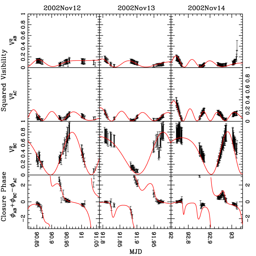
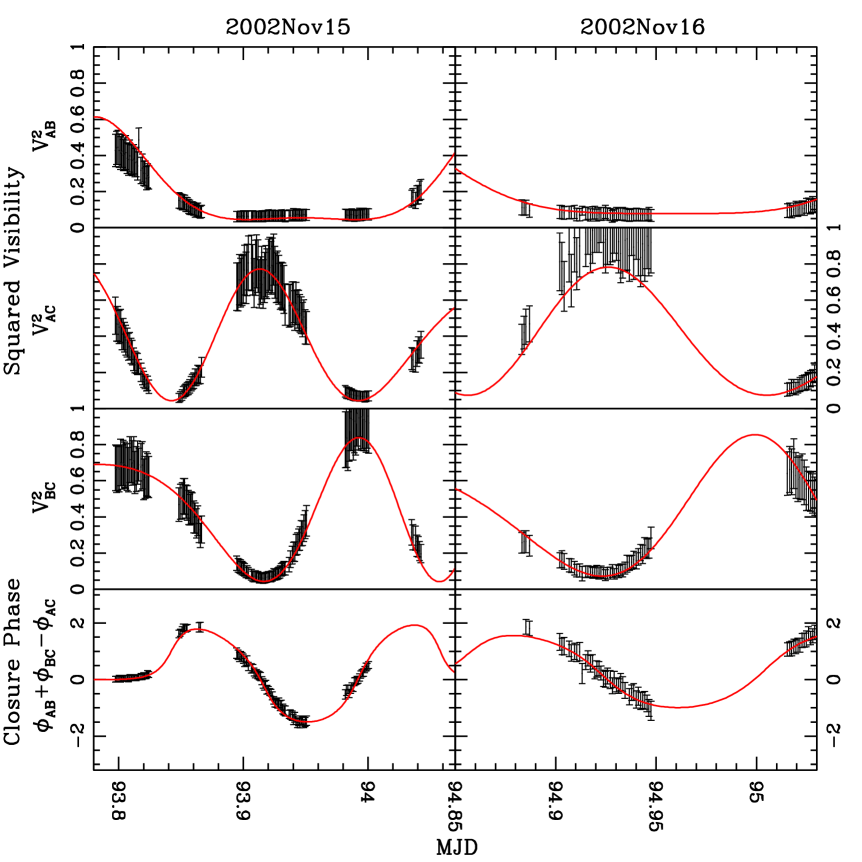
The fit results for each individual night are given in Table 2 and Figures 2 and 3. In some cases, the reduced $\chi^{2}$ values exceed unity, which might be a result of bad seeing, a potentially uncorrected bias due to the effect of bandwidth smearing, the piezo scanner resonances, or other undiscovered systematic errors. However, the measurements are clearly in good agreement with the high precision reference orbit by Hummel et al. (1994) obtained with two telescopes on the Mark III interferometer.

Weighted averaging give for the diameters of the Capella giants, $\Theta_{Aa}=8.9\pm 0.6$ mas and $\Theta_{Ab}=5.8\pm 0.8$ mas and the intensity ratio $I_{Aa}/I_{Ab}=1.49\pm 0.10$. Using the orbital parallax of $75.0\pm 0.57$ mas (Pourbaix, 2000) we calculate physical radii of $R_{Aa}=12.6\pm 0.9$ $R_{\sun}$ and $R_{Ab}=8.3\pm 1.1$ $R_{\sun}$.

Stellar radii measurements are of special importance as the most direct way to determine stellar effective temperatures. The stellar radii, derived from our $H$-band data, are in good agreement with the measurements at visible wavelengths by Hummel et al. (1994). As a result of our longer effective wavelength and the smaller amount of data, we cannot exceed the precision of their extensive study. Therefore, we skip re-calculating the effective temperatures with our values.

5 Imaging

Figure 4: Image reconstructions from subsets of our complete data set revealing the orbital motion of the stars between three epochs. To compensate the marginal motion within the subsets, the $u,v$-plane was rotated synchronously to the reference position of the components at the intermediary modified julian dates MJD=$91.437$, $93.907$ and $94.262$ (MJD=JD$-$2452500). The crosses within the maps indicate the “centers of light” of the stars within the other images. Whereas the positions fit the expectations accurately ($\leq 1$ mas), the intensity ratio between the two stars was not always obtained properly due to the poor sampling (the coverage is shown below each map). The contours show $10\%$ intervals scaled to the peak.

Figure 5: Aperture synthesis maps of Capella generated with data from 2002 Nov 12-16. Maps generated with the CHM (upper left), DFM (upper right), and BBM (lower left) algorithm are shown together with the $u,v$-plane coverage (lower right). Each map shows the surface brightness plotted with $5\%$ interval contours (scaled to the peak intensity). To compensate for the motion of the stars over the observed interval ($\approx 14\arcdeg$), the $u,v$-plane was moved synchronously to the orbital motion. The maps are oriented north up, east left. The restoring beam ($5.4\times 2.6$ mas) is shown in the upper-left corner of each map as inset.

5.1 Imaging Algorithms used

In the exploratory spirit of the present Capella imaging work, we have investigated three different imaging algorithms, as explained here.

The radio astronomy community has developed various algorithms to reconstruct phase information from CP, most notably conventional hybrid mapping (CHM, e.g. Cornwell and Wilkinson, 1981) and difference mapping (DFM) by Pearson et al. (1994). In both algorithms, the individual phases are recovered by self-calibration (Pearson and Readhead, 1984). The necessary deconvolutions can be performed with the classical CLEAN algorithm (e.g. Högbom, 1974).

We have also tested the “building-block mapping” (BBM) algorithm presented by Hofmann and Weigelt (1993), which was originally developed to reconstruct images from speckle-bispectrum data. Here, the image is build up by adding iteratively point-like components (building blocks) to an image in order to minimize the least square distance between the measured bispectrum and the bispectrum of the reconstructed image. Since the computation of this distance function for each potential position of the next building block (the whole image space) is computationally too expensive, a linear approximation of the least square distance is applied. The main assumption of this approximation is that the added component changes the bispectrum of the reconstructed image only insignificantly. For details of this method, see Hofmann and Weigelt (1993).

In order to allow a comparison of the results obtained with the various methods, we implemented all algorithms within one software framework. This allows us to start all image reconstruction methods with precisely the same initial conditions.

5.2 Mapping the orbital motion

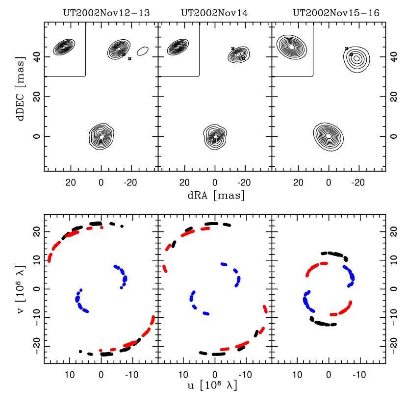
To demonstrate that the data and mapping techniques were sensitive to the movement of the stars during the observation period, we subdivided our data into three subsets (2002 Nov 12-13, 2002 Nov 14, 2002 Nov 15-16), each one still containing enough data for mapping. Since we observed during the first two epochs with the telescope configuration including the longest baseline (and hereby missing lower frequencies), the convergence of the BBM maps had to be supported by limiting the reconstruction area. Within the maps generated (Fig. 4) it is perceivable that the orbital motion can clearly be traced accurately. Also the intensity of the stars (from left to right: $I_{Aa}/I_{Ab}\approx$ 1.6, 1.7, 1.6) can be estimated reliably.

5.3 Compensating the orbital motion

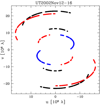
The key goal of our project was to produce aperture synthesis images of Capella in order to demonstrate the capabilities of IOTA/IONIC3. However, observations were obtained over five nights, during which time the relative positions of the binary pair changed by many milliarcseconds. In order to make a single map with data from all nights, and thereby improve the $u,v$ coverage available for the map, we applied a coodinate transformation to compensate for the orbital motion of the binary components over the observed time interval. Thus, the fringe spacing is rescaled to account for the changing separation of the stars, and the orientation of the fringes on the sky is reoriented to account for the changing position angle of the binary pair. Each $u,v$ point was transformed in this manner to a new coordinate system corresponding to the geometry of the stars at the time of the middle of our observation run. This way, all observations may be combined to produce a single map with improved $u,v$ coverage.

Of course, the above procedure is only strictly justified for special circumstances. In a binary system, the stars would have to rotate synchronously and any brightness structure on each star would have to be stationary during the time of observation. In the Capella system, we note that this procedure might be justified for the cooler Aa component, which has been found to rotate synchronously to the orbital motion (Strassmeier et al., 2001). The infrared-fainter Ab component rotates asynchronously, hence it would not be possible to map structure onto this more active star.

The resulting CHM, DFM and BBM maps are presented in Fig. 5. For the given, sufficient simple brightness source distribution, all algorithms converged without any concrete trial model assumptions or other specific pre-suppositions. As an initial phase estimate we set two of the three phases equal to zero, thus the third phase was given by the closure phase relation. The intensity ratios $I_{Aa}/I_{Ab}$ measured within the maps are 1.9 (CHM), 1.6 (DFM), and 1.8 (BBM).

A quantitative comparison between the BBM map in Fig. 5 and the maps constructed from the data subsets as described in chapter 5.2 reveals that the rotation compensating coordinate transformation clearly reduced the noise content within the maps and also improved the convergence behaviour.

Since the stellar surfaces within the maps are partially resolved, one can measure the stellar diameters. This provides values of $\Theta_{Aa}^{\textnormal{map}}=8.3\pm 1.6$ and $\Theta_{Ab}^{\textnormal{map}}=6.8\pm 1.2$ (measured within the unconvolved BBM map), which is in good agreement with our model fitting results.

6 Conclusions

By observing the well-studied Capella system we were able to demonstrate the overall performance and imaging capabilities of the IOTA/IONIC3 instrument. IOTA was able to successfully measure and calibrate visibility amplitudes and closure phases, even with a temporary but significant instrumental problem that affected the raw data adversely during this run. The visibility amplitudes and closure phases were then used with three algorithms to reconstruct reliable images of this well known binary system. Thus, the primary goal of this experiment has been achieved, and the IOTA facility has been shown to be a powerful tool for high-resolution infrared imaging.

Acknowledgement. S.K. was supported by NSF grant AST-0138303 and the International Max Planck Research School (IMPRS) for Radio and Infrared Astronomy at the University of Bonn.

References

- Anderson (1920) Anderson, J. A.: 1920, ApJ 51, 263
- Baldwin et al. (1996) Baldwin, J. E., Beckett, M. G., Boysen, R. C., Burns, D., Buscher, D. F., Cox, G. C., Haniff, C. A., Mackay, C. D., Nightingale, N. S., Rogers, J., Scheuer, P. A. G., Scott, T. R., Tuthill, P. G., Warner, P. J., Wilson, D. M. A., and Wilson, R. W.: 1996, A&A 306, L13+
- Berger et al. (2003) Berger, J., Haguenauer, P., Kern, P. Y., Rousselet-Perraut, K., Malbet, F., Gluck, S., Lagny, L., Schanen-Duport, I., Laurent, E., Delboulbe, A., Tatulli, E., Traub, W. A., Carleton, N., Millan-Gabet, R., Monnier, J. D., and Pedretti, E.: 2003, in Interferometry for Optical Astronomy II. Edited by Wesley A. Traub . Proceedings of the SPIE, Volume 4838, pp. 1099-1106 (2003)., pp 1099–1106
- Campbell (1899) Campbell, W. W.: 1899, ApJ 10, 177
- Cornwell and Wilkinson (1981) Cornwell, T. J. and Wilkinson, P. N.: 1981, MNRAS 196, 1067
- Coudé Du Foresto et al. (1997) Coudé Du Foresto, V., Ridgway, S., and Mariotti, J.-M.: 1997, A&AS 121, 379
- Högbom (1974) Högbom, J. A.: 1974, A&AS 15, 417
- Hofmann and Weigelt (1993) Hofmann, K.-H. and Weigelt, G.: 1993, A&A 278, 328
- Hummel et al. (1995) Hummel, C. A., Armstrong, J. T., Buscher, D. F., Mozurkewich, D., Quirrenbach, A., and Vivekanand, M.: 1995, AJ 110, 376
- Hummel et al. (1994) Hummel, C. A., Armstrong, J. T., Quirrenbach, A., Buscher, D. F., Mozurkewich, D., Elias, N. M., and Wilson, R. E.: 1994, AJ 107, 1859
- Jennison (1958) Jennison, R. C.: 1958, MNRAS 118, 276
- Johnson et al. (2002) Johnson, O., Drake, J. J., Kashyap, V., Brickhouse, N. S., Dupree, A. K., Freeman, P., Young, P. R., and Kriss, G. A.: 2002, ApJ 565, L97
- Monnier (2001) Monnier, J. D.: 2001, PASP 113, 639
- Monnier et al. (2004) Monnier, J. D., Traub, W. A., Schloerb, F. P., Millan-Gabet, R., Berger, J.-P., Pedretti, E., Carleton, N. P., Kraus, S., Lacasse, M. G., Brewer, M., Ragland, S., Ahearn, A., Coldwell, C., Haguenauer, P., Kern, P., Labeye, P., Lagny, L., Malbet, F., Malin, D., Maymounkov, P., Morel, S., Papaliolios, C., Perraut, K., Pearlman, M., Porro, I. L., Schanen, I., Souccar, K., Torres, G., and Wallace, G.: 2004, ApJ 602, L57
- Pearson and Readhead (1984) Pearson, T. J. and Readhead, A. C. S.: 1984, ARA&A 22, 97
- Pearson et al. (1994) Pearson, T. J., Shepherd, M. C., Taylor, G. B., and Myers, S. T.: 1994, Bulletin of the American Astronomical Society 26, 1318
- Pedretti et al. (2004) Pedretti, E., Millan-Gabet, R., Monnier, J. D., Traub, W. A., Carleton, N. P., Berger, J.-P., Lacasse, M. G., Schloerb, F. P., and Brewer, M. K.: 2004, PASP 116, 377
- Pourbaix (2000) Pourbaix, D.: 2000, A&AS 145, 215
- Richichi and Percheron (2002) Richichi, A. and Percheron, I.: 2002, A&A 386, 492
- Ségransan et al. (2003) Ségransan, D., Kervella, P., Forveille, T., and Queloz, D.: 2003, A&A 397, L5
- Strassmeier et al. (2001) Strassmeier, K. G., Reegen, P., and Granzer, T.: 2001, Astronomische Nachrichten 322, 115
- Torrence and Compo (1998) Torrence, C. and Compo, G. P.: 1998, Bulletin of the American Meteorological Society 79(1), 61
- Traub et al. (2003) Traub, W. A., Ahearn, A., Carleton, N. P., Berger, J., Brewer, M. K., Hofmann, K., Kern, P. Y., Lacasse, M. G., Malbet, F., Millan-Gabet, R., Monnier, J. D., Ohnaka, K., Pedretti, E., Ragland, S., Schloerb, F. P., Souccar, K., and Weigelt, G.: 2003, in Interferometry for Optical Astronomy II. Edited by Wesley A. Traub. Proceedings of the SPIE, Volume 4838, pp. 45-52 (2003)., pp 45–52
- Young (1999) Young, J. S.: 1999, Ph.D. thesis, St. John’s College, Cambridge and Cavendish Astrophysics