Solutions for 10,000 Eclipsing Binaries in the Bulge Fields of OGLE II Using DEBiL

Abstract

We have developed a fully-automated pipeline for systematically identifying and analyzing eclipsing binaries within large datasets of light curves. The pipeline is made up of multiple tiers which subject the light curves to increasing levels of scrutiny. After each tier, light curves that did not conform to a given criteria were filtered out of the pipeline, reducing the load on the following, more computationally intensive tiers. As a central component of the pipeline, we created the fully automated Detached Eclipsing Binary Light curve fitter (DEBiL), which rapidly fits large numbers of light curves to a simple model. Using the results of DEBiL, light curves of interest can be flagged for follow-up analysis. As a test case, we analyzed the 218699 light curves within the bulge fields of the OGLE II survey and produced 10862 model fits. We point out a small number of extreme examples as well as unexpected structure found in several of the population distributions. We expect this approach to become increasingly important as light curve datasets continue growing in both size and number.

1 Introduction

Light curves of eclipsing binary star systems provide the only known direct method for measuring the radii of stars without having to resolve their stellar disk. These measurements are needed for better constraining stellar models. This is especially important for such cases as low-mass dwarfs, giants, pre-main sequence stars and stars with non-solar compositions, for which we currently have a remarkably small number of well-studied examples. Other important benefits of locating binary systems include more accurate calibration of the local distance ladder (Paczynski, 1996; Kaluzny et al., 1998), constraining the low mass IMF, and discovering new extrasolar planets. In order to obtain measurements of the stars’ radii and masses, one needs to incorporate both the light curve (photometric observations) and radial velocities (spectroscopic observations) of the system. Since making large-scale spectroscopic surveys is significantly more difficult than making photometric surveys, it is far more efficient to begin with a photometric survey and later follow-up with spectroscopic observation only on systems of interest.

During the past decade, there have been numerous light curve surveys (e.g. OGLE: Udalski et al. (1994); EROS: Beaulieu et al. (1995); DUO: Alard & Guibert (1997); MACHO: Alcock et al. (1998)) that take advantage of advances in photometric analysis, such as difference image analysis (Crotts, 1992; Phillips & Davis, 1995; Alard & Lupton, 1998). The original goal of many of these surveys was not to search for eclipsing binaries, but rather to search for gravitational microlensing events (Paczynski, 1986). Fortunately, the data derived from these surveys are ideal for eclipsing binary searches as well. More recently, there have also been mounting efforts to create automated light curve surveys (e.g. ROTSE: Akerlof et al. (2000); HAT: Bakos et al. (2004) ; TrES: Alonso et al. (2004)) using small robotic telescopes for extrasolar planet searches. The upcoming large synoptic surveys (e.g. Pan-STARRS: Kaiser et al. (2002); LSST: Tyson (2002)), spurred by the decadal survey of the National Academy of Sciences, are expected to dwarf all the surveys that precede them. Put together, these surveys provide an exponentially growing quantity of photometric data (Szalay & Gray, 2001), with a growing fraction becoming publicly available.

2 Motivation

For over 30 years many codes have been developed with the aim of fitting increasingly complex models to eclipsing binary light curves (e.g. Wilson & Devinney (1971); Nelson & Davis (1972); Wilson (1979); Etzel (1981)). These codes have had great success at accurately modeling the observed data, but also require a substantial learning curve to fully master their operation. The result is that up till now there have been no comprehensive catalogue of reliable elements for eclipsing binaries (Cox, 2000).

In order to take full advantage of the large-scale survey datasets, one must change the traditional approach of manual light curve analysis. The traditional method of painstakingly fitting models one by one is inherently limited by the requirement of human guidance. Ideally, fitting programs should be both physically accurate and fully automated. Many have cautioned against full automation (Popper, 1981; Etzel, 1991; Wilson, 1994) since it is surprisingly difficult, without the aid of a human eye, to recognize when a fit is “good”. In addition, it is essentially impossible to resolve certain parameter degeneracies without a priori knowledge and extensive user experience. Despite these challenges, there have been a small number of pioneering attempts at such automated programs (Wyithe & Wilson, 2001, 2002). However, the large numerical requirements of these programs make it computationally expensive to perform full fits (i.e. without having some parameters set to a constant) of large-scale datasets. Moore’s law, which stated in effect that CPU speed doubles every 18 months, cannot in itself solve this problem, since the quantity of data to be analyzed is also growing at a similar exponential rate (Szalay & Gray, 2001). Instead, we advocate replacing the approach of using monolithic automated fitting programs with a multi-tiered pipeline (fig. 1). In such a pipeline, a given light curve is piped through a set of programs that analyze it with increasing scrutiny at each tier. Light curves that are poorly fit or don’t comply with set criteria are filtered out of the pipeline, thus passing a far smaller number of candidates on to the following, more computationally demanding tier. Such a pipeline, coupled with efficient analysis programs, can increase the effective speed of fitting models by a few orders of magnitude compared to monolithic fitting programs. This approach makes it practical to perform full fits of the largest light curve datasets, with only moderate computational resources. Using a single-CPU SUN UltraSPARC 5 workstation (333 MHz), the average processing time of our pipeline was $\sim$1 minute per light curve. Where each light curve typically contains a few hundred photometric observations. We must emphasize that even at these speeds, we still need a few CPU-months to fully process an OGLE-like survey containing $10^{5}$ light curves. In about a decade, the large synoptic surveys are slated to create datasets that are more than 4 orders of magnitude larger than that (Tyson, 2002).

The Detached Eclipsing Binary Light curve fitter (DEBiL) is a program we created to serve as an intermediate tier for such a multi-tiered pipeline. DEBiL is a fully automated program for fitting eclipsing binary light curves, designed to rapidly fit a large dataset of light curves in an effort to locate a small subset that match given criteria. The matched light curves can then be more carefully analyzed using traditional fitters. Conversely, one can use DEBiL to filter out the eclipsing binary systems, in order to study other periodic systems (e.g. spotted or pulsating stars). In order to achieve speed and reliable automation, DEBiL employs a simple model of a perfectly detached binary system: limb darkened spherical stars with no reflections or third light, in a classical 2-body orbit. Given the system’s period and quadratic limb darkening coefficients (the default is solar limb darkening), the DEBiL fitter will fit the following eight parameters:

• Radius of primary star

• Radius of secondary star

• Brightness of primary star

• Brightness of secondary star

• Orbital eccentricity

• Orbital inclination

• Epoch of periastron

• Argument of periastron

Since we don’t have an absolute length-scale, we measure both stars’ radii as a fraction of the sum of their orbital semimajor axes (a).

This simple model allows the use of a nimble convergence algorithm that is comprised of many thousands of small steps that scour a large portion of the problem’s phase space. Admittedly, this model can only give a crude approximation for semidetached and contact binaries, but it can easily identify such cases and can flag them for an external fitting procedure. In addition to pipeline filtration, DEBiL can also provide an initial starting guess for these external fitters, a task that usually has to be performed manually.

3 Method

This section describes our implementation of a multi-tiered light curve-fitting pipeline. We fine-tuned and tested our design using light curves from the bulge fields of the second phase Optical Gravitational Lensing Experiment (OGLE II) (Udalski et al., 1997; Wozniak et al., 2002). Our resulting pipeline consists of the following six steps:

First tier: Periodogram

1. Find the light curve period

2. Filter out non-periodic light curves

Second tier: DEBiL

1. Find an “initial guess” for the eclipsing binary model parameters

2. Filter out non-eclipsing systems (i.e. pulsating stars)

3. Numerically fit the parameters of a detached eclipsing binary model

4. Filter out unsuccessful fits

For OGLE II data, we found that about half of the total CPU-time was spent on step (1) and about half on step (5). The remaining steps required an insignificant amount of CPU-time. Note that step (5), which typically takes more than 10 times longer to run than step (1), was only run on less than $10\%$ of the light curves. By filtering out more than $90\%$ of the light curves at earlier steps, the pipeline was able to run $\sim$10 times faster than it would have been able to otherwise. Both steps (1) and (5) can themselves be speeded up, but at a price of lowering their reliability and accuracy. The third tier, in which the light curves of interest are fitted using physically accurate models, is dependent on the research question being pursued and won’t be further discussed here.

3.1 The First Tier – Finding the Period

Step (1) is performed using an “off-the-shelf” period search technique. All the periodogram algorithms that we have tested give comparable results, and we adopted an analysis of variance (Schwarzenberg-Czerny, 1989, 1996) as it appears to do a good job handling the aliasing in OGLE light curves. In our implementation, we scanned periods from 0.1 days up until the full duration of the light curve ($\sim$1000 days for OGLE II). We then selected the period that minimizes the variance around a second order polynomial fit within 8 phase bins. Aliases pose a serious problem for period searches since they can prevent the detection of weak periodicities, or periods that are close to an alias. The “raw” period distribution of the OGLE II light curves showed aliases with a typical widths ranging from 0.001 days for the shortest periods, up to 0.04 days for longest periods. We suppressed the 12 strongest aliases, over which the results were dominated by false positives, and had the period finder return the next best period. Fewer than $1\%$ of the true light curve periods are expected to have been affected by this alias suppression. Finally, once a period was located, rational multiples of it, with numerators and denominators of 1 through 19 were also tested to see if they provide better periods.

Step (2) filters out all the light curves that aren’t periodic. The analysis of variance from step (1) provides us with a measure of “scatter” in a light curve, after being folded into a given period. Ideally, when the period is correct, the folded data are neatly arranged, with minimal scatter due to noise. In contrast, when the light curve is folded into an incorrect period, the data are randomized and the scatter is increased. In order to quantify this, we measure the amount of scatter in each of the tested periods, and calculate the number of sigmas the minimum scatter is from the mean scatter. We call this quantity, the periodic strength score. In an attempt to minimize the number of non-eclipsing binaries that continue to the next step, while maximizing the number of eclipsing binaries that pass through, we chose a minimum periodic strength score cutoff of 6.5. In addition to this, we set a requirement that the variables’ period be no longer than 200 days, which guarantees at least four foldings. These two criteria filtered out approximately $90\%$ of all the light curves in OGLE II dataset.

In order to test the effectiveness of these filtration criteria, we measured the filtration rates for field 33, a typical OGLE II bulge field (fig. 2). We then repeated this measurement for a range of periodicity strength cutoffs (the 200-day criterion remained unchanged). For periodicity strength cutoffs up to 4, there is a sharp reduction in the number of systems, as non-variable light curves are filtered out. Users should be aware that constant light curves can be well-fit by degenerate DEBiL models. By filtering out systems with such low periodicity strength we correctly remove these systems, and in so doing noticeably lower the total number of well-fitted systems. Raising the filtration cutoff, up until about 6.5, will continue reducing the filter-through rate, but with only a small impact on the number of well-fit systems. Further raising the cutoff will begin again reduce number of fitted systems, this time removing good systems. We may conclude from this test that the optimal periodicity strength cutoff is between 4 and 6.5, so that non-variable systems are mostly filtered out while eclipsing binaries are mostly filtered through. Since the filter-through rate monotonically decreases as the cutoff is raised, the pipeline becomes significantly more computationally efficient at the high end of this range, thus bringing us to our cutoff choice of 6.5. Users with more computing power at their disposal may consider lowering the cutoff to the lower end of this range. In so doing they slightly reduce the risk of filtering out eclipsing binaries, at the price of significantly lowering the pipeline computational efficiency.

3.2 The Second Tier – DEBiL Fitter

Steps (3) through (5) are performed within the DEBiL program. Step (3) provides an “initial guess” for the model parameters. It identifies and measures the phase, depth and width of the two flux dips which occur in each orbit. Using a set of equations that are based on simplified analytic solutions for detached binary systems (Danby, 1964; Mallén-Ornelas et al., 2003; Seager & Mallén-Ornelas, 2003), DEBiL produces a starting point for the fitting optimization procedure. Step (4) filters out light curves with out-of-bound parameters, so to protect the following step. In practice this step is remarkably lax. It typically filters out only a small fraction of the light curves that pass through it, but those that are filtered out are almost certain not to be eclipsing binaries. Step (5) fits each light curve to the 8-parameter DEBiL model (see §2), fine-tunes it, and estimates its parameter uncertainties. This step starts with the light curve that would have been seen with the “initial guess” parameters. It then systematically varies the parameters according to an optimization algorithm, so as to minimize the square of the residuals in an attempt to converge to the best fit. The optimization algorithm chosen for the DEBiL fitter is the downhill simplex method combined with simulated annealing (Nelder, 1965; Kirkpatrick et al., 1983; Vanderbilt & Louie, 1983; Otten & van Ginneken, 1989; Press et al., 1992). This algorithm was selected for its simplicity, speed and its relatively long history at reliably solving similar problems, which involve locating a global minimum in a high-dimensional parameter-space. Other methods that were considered are gradient-based (Press et al., 1992) and genetic algorithms (Holland, 1992; Charbonneau, 1995). Gradient-based (steepest descent) algorithms can converge very quickly to a local minimum, but are not designed for finding the global minimum. In addition, the difficulty in calculating the gradient of non-analytic function slows these algorithms considerably and causes them to be less robust. Genetic algorithms provide a promising new approach for locating global minima, with the unique advantage of being parallelizable. Unfortunately, their implementations are more complicated, while not having a significant advantage in speed or reliability over the downhill simplex method.

Determining a convergence threshold at which to stop optimization algorithms is known to be a hard problem (Charbonneau, 1995). This is because the convergence process of these algorithms will go through fits and stops. The length of the “stops”, whereby the convergence does not significantly improve, becomes longer with time, ultimately approaching infinity. Since there is no known way to generally predict these fits and stops, we chose simply to have the algorithm always run for 10,000 iterations (can be adjusted at the command line). This number was found to be adequate for OGLE light curves (see §4), with larger numbers not showing a significant improvement in the convergence. Using a constant number of iterations has the significant benefit of enabling the user to make accurate predictions of the total computing time that will be required. At the end of the 10,000 iterations, the best solution encountered so far is further fine-tuned, so to guarantee that it is very close to the bottom of the current minimum. In our implementation we make sure every parameter is within $0.1\%$ of the minimum ($p_{min}$).

Finally, DEBiL attempts to estimate the uncertainties of the fitted parameters. This is done by perturbing each parameter by a small amount ($\Delta p$) and measuring how sensitive the model’s reduced chi square ($\chi_{\nu}^{2}$) is to that parameter. In our implementation we set the perturbation to be $0.5\%$ of $p_{min}$. At each parameter perturbation measurement, the remaining parameters are re-fine-tuned, so to take into account the parameters’ covariances. We then use a second order Taylor expansion to derive the second derivative of $\chi_{\nu}^{2}$ at the minimum, which is used to extrapolate the local shape of the $\chi_{\nu}^{2}$-surface:

$$\chi_{\nu}^{2}\left(p_{min}+\Delta p\right)\simeq\chi_{\nu}^{2}\left(p_{min}\right)+\frac{1}{2}\cdot\frac{\partial^{2}\chi_{\nu}^{2}}{\partial p_{min}^{2}}\cdot\left({\Delta p}\right)^{2}$$ (1)

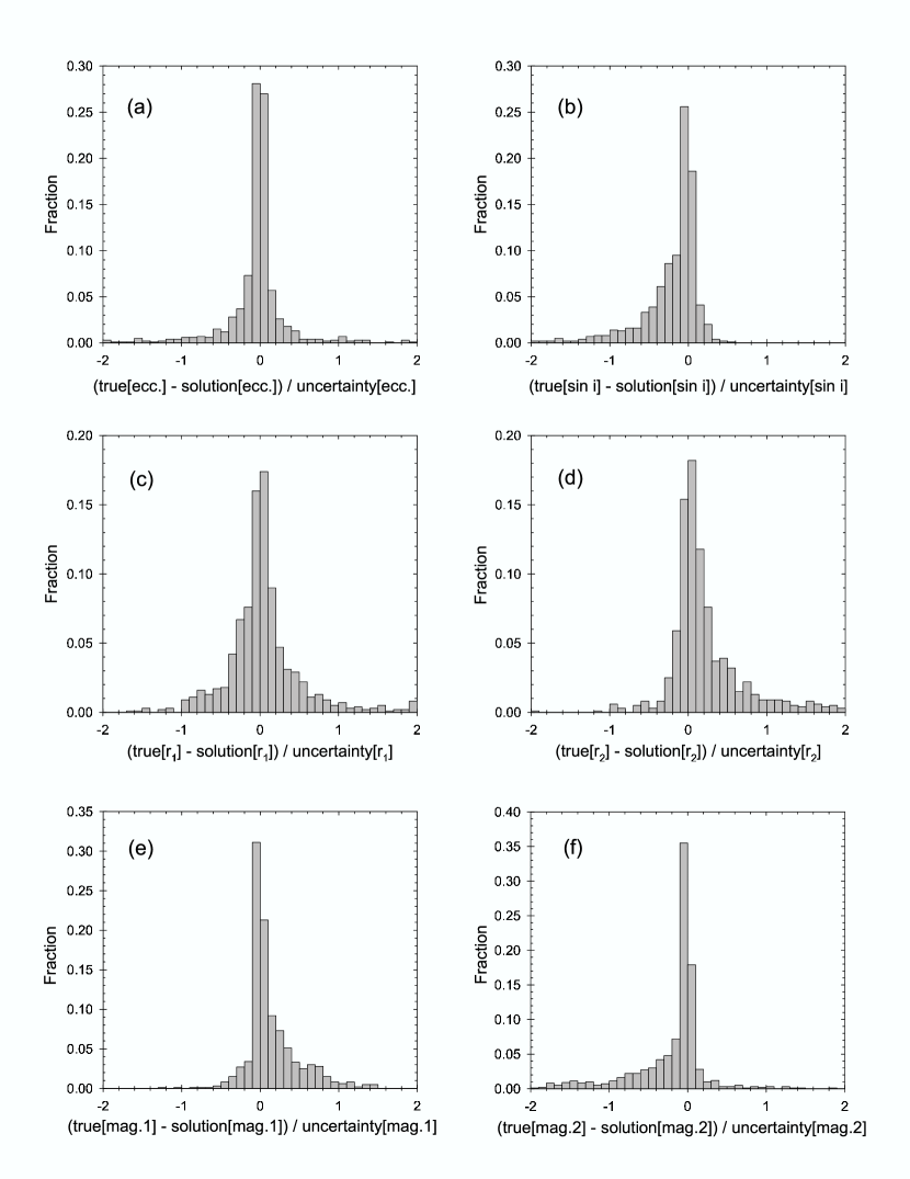
Figure 3: Histograms of the error distribution in DEBiL fitted parameters. This plot was created by fitting 1000 simulated eclipsing light curves with 5% Gaussian photometric noise. The fitting error of each parameter was normalized by its estimated uncertainty (as defined in §3.2). The distributions seen here are not Gaussian, but rather have a slender peak, and long tails (i.e. large kurtosis). The distributions also have varying degrees of skewness, which is discussed in §3.3.

We chose to employ a non-standard definition for the DEBiL parameter uncertainties, which seems to describe the errors of all the fitted parameters (fig. 3) far better than the standard definition (Press et al., 1992). In the standard definition, the uncertainty of a parameter is equal the size of the perturbation from the parameter’s best-fit value, which will raise $\chi_{\nu}^{2}$ by $1/\nu$, while fitting the remaining parameters. The reasoning behind this definition implicitly assumes that $\chi_{\nu}^{2}$ is a smooth function. But in fact the $\chi_{\nu}^{2}$-surface of this problem is jagged with numerous local minima. These minima will fool the best attempts at converging to the global minimum and cause the parameter errors to be far larger than the standard uncertainty estimate would have us believe. For this reason we adopted a non-standard empirical definition for the parameter uncertainties ($\varepsilon_{p}$). In our variant, the uncertainty of a parameter is equal the size of the perturbation from the parameter’s best-fit value, which will double $\chi_{\nu}^{2}$, while fitting the remaining parameters:

$$\chi_{\nu}^{2}\left(p_{min}+\varepsilon_{p}\right)=2\chi_{\nu}^{2}\left(p_{min}\right)$$ (2)

This definition assigns larger uncertainties to more poorly-fit models. In addition, it is insensitive to systematic over- or under-estimated photometric uncertainties, which are all too common in many light curve surveys. Using the previous two equations, we can estimate $\varepsilon_{p}$ as:

$$\varepsilon_{p}\simeq{\Delta p\cdot\sqrt{\frac{\chi_{\nu}^{2}\left(p_{min}\right)}{\chi_{\nu}^{2}\left({p_{min}+\Delta p}\right)-\chi_{\nu}^{2}\left(p_{min}\right)}}}$$ (3)

Note that the standard uncertainty is approximately: $\varepsilon_{p}/\sqrt{\chi^{2}}$ , so users can easily convert to it, if so desired.

Step (6) is the final gatekeeper of our pipeline. It evaluates the model solutions and filters out all but the “good” models according to some predefined criteria. DEBiL users are expected to configure this step so to fit the particular needs of their research. To this end, DEBiL provides a number of auxiliary tests designed to quantify how well the model fits the data. Reduced chi-square and fitness score values measure the overall quality of the fit, while scatter score and waviness values measure local systematic departures of the model from the data (see appendix A).

Additional filtering criteria are usually needed in order to remove non-eclipsing-binary light curves that have either (a) overestimated uncertainties that produce low reduced chi-square results, or (b) look deceptively similar to eclipsing binary light curves. Filtration criteria should be placed with great care in order to minimize filtering out “good” light curves. In order to handle overestimated uncertainties (a), one can filter out models with low fitness score. Handling non-eclipsing-binary light curves that look like binary light curves (b) is considerably more difficult. Many of these problematic light curves are created by pulsating stars (e.g. RR-Lyrae type C), which have sinusoidal light curves that resemble those of contact binaries. To this end, DEBiL also provides the reduced chi-square of a best-fit sinusoidal function of each light curve. If this value is similar or lower than the model’s reduced chi-square, then is it likely that the light curve indeed belongs to a pulsating star.

3.3 Limitations

In the previous subsection we discussed the considerable difficulties in finding the global minimum in the jagged structure of the $\chi_{\nu}^{2}$-surface. At this point we must further add, that since the data is noisy and the model is imperfect, the true solution might not be at the global minimum. For the lack of better information, we can only use the global minimum as the point in parameter-space that is the most likely to be the true solution.

Another source of errors are systematic fitting biases, which must especially be taken into account when making detailed population studies. Two main sources of these biases are imperfect models and asymmetric $\chi_{\nu}^{2}$-minima. Almost all models are imperfect, but when effects not included in the model become significant, the optimization algorithm will often try to compensate for this by erroneously skewing some of the parameters within the model. An example of this is seen in semidetached binaries. The tidal distortions of these stars are not modeled by DEBiL, so as a result DEBiL will compensate for this by overestimating their radii. Most model imperfections are flagged by a large reduced chi-square. Surprisingly, for tidal distortions, the reduced chi-square is not significantly increased. For this reason we provide a “detached system” criterion that will be described in §5. The effects of asymmetric $\chi_{\nu}^{2}$-minima are more subtle. In such cases a perturbation to one side of a $\chi_{\nu}^{2}$-minimum raises $\chi_{\nu}^{2}$ less than a perturbation to the other side. Thus random noise in the data will cause the parameters to be systematically shifted more often in the former direction than in the latter. We believe that these biases, which are universal to all fitting programs, can be corrected after the fact. We chose not to do this in order to avoid having to insert any fudge factors into DEBiL. But we acknowledge that this may be necessary in order to extend the regimes in which DEBiL is reliable without significantly reducing its speed.

Possibly the most problematic fitting errors are those that are caused by mistaken light curve periods. For eclipsing binaries with strong periodicity scores, the main cause of this is the confusion between two types of light curves: (a) light curves with very similar and equally-spaced eclipses, and (b) light curves with an undetected eclipse. Both these types of light curves will appear to have a single eclipse in their phased light curve. Light curves with similar eclipses (a) will cause the period finder to return a period that is half the correct value, folding the primary and secondary eclipse over one another. In contrast to this, light curves with an undetected eclipse (b), either because it’s hidden within the noise or because it’s in a phase coverage gap, will have the correct period. Because the undetected eclipse is necessary for determining a number of the fitting parameter, we are not able to model this type of light curve. Fortunately, light curves with similar eclipses (a) can be easily modeled by simply doubling their period. Since we can’t generally distinguish between these two types of light curves, the DEBiL fitter treats all the single-eclipse light curves as type (a), doubling their period and fitting them as best it can. Whenever such a period-doubling occurs, DEBiL inserts a warning message into the log file. These light curves should be used with increased scrutiny. This problem is further compounded in surveys, such as the OGLE II bulge fields, which consist of many non-eclipsing-binary variables. As mentioned in §3.2, some of these systems look deceptively similar to eclipsing binaries. Since their brightness oscillation typically consists of a single minima, they too will have their period doubled. In conclusion, unless the systems with doubled periods are filtered out, there will be an erroneous excess of light curves with similar primary and secondary eclipses. In turn, this will manifests itself in an excess of model solutions with stars of approximately equal surface brightness.

Even though our discussions of possible causes and remedies for limitations stemmed from our experience with our particular pipeline, many of these points are also likely to apply to other similar pipelines and fitting procedures.

4 Tests

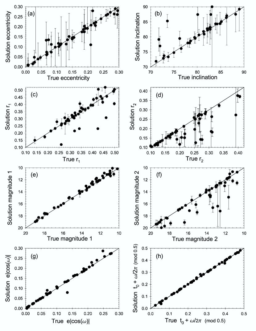
Figure 4: The fitted solutions versus the true solution in 50 simulated eclipsing binary light curves with Gaussian photometric noise of 1%. We simulated a uniform distribution of parameters, with the only requirement being that both eclipse dips were detectable through the noise. Panels (a) through (f) show the fits of DEBiL model parameters with their uncertainties, as defined in §3.2. Panels (g) and (h) combine parameters so that they describe prominent features of the light curve (respectively, the separation and offset of the eclipse centers). In these combination, the parameter errors largely cancel out, so that the formal uncertainties should not be used.

In order to test the DEBiL fitter, we ran it both on simulated light curves and published, fully analyzed, observed light curves (Lacy et al., 2000, 2002, 2003). Figure 3 shows the results of fitting 1000 simulated light curve, with $5\%$ Gaussian photometric noise. Figure 4 provides a more detailed look at the fits to 50 simulated light curves, with $1\%$ Gaussian photometric noise, giving results comparable to those of Wyithe & Wilson (2001). Not surprisingly, when less noise was inserted into the light curve, the fitter estimated considerably smaller uncertainties.

While the simulated light curves are easy to produce and have known parameter values, observed light curves are the only ones that can provide a true reality check. To this end, we also reanalyze three published light curves (fig. 5):

• Table 1: FS Monocerotis (Lacy et al., 2000)

• Table 2: WW Camelopardalis (Lacy et al., 2002)

• Table 3: BP Vulpeculae (Lacy et al., 2003)

We present here a comparison between the aforementioned published photometric fits, using the Nelson-Davis-Etzel model implemented by EBOP (Etzel, 1981; Popper & Etzel, 1981) and the DEBiL fits. For all three cases, we used the V-band observational data and set DEBiL’s limb darkening quadratic coefficients to the solar V-band values (Claret, 2003). We found that when applying the physically correct limb darkening coefficients, the improvements in the best-fit model were negligible compared to the uncertainties. For this reason, we chose to use solar limb darkening coefficients throughout this project.

5 Results

We used the aforementioned pipeline to identify and analyze the eclipsing binary systems within the bulge fields of OGLE II (Udalski et al., 1997; Wozniak et al., 2002). The final result of our pipeline contained only about 5% of the total number of light curves we started with. The filtration process progressed as follows:

• Total number of OGLE II (bulge fields) variables: 218699

• After step (2), with strong periodicity and periods of 0.1-200 days: 19264

• After step (4), the output of the DEBiL program: 17767

• After step (6), with acceptable fits to binary models ($\chi_{\nu}^{2}<4$): 10862

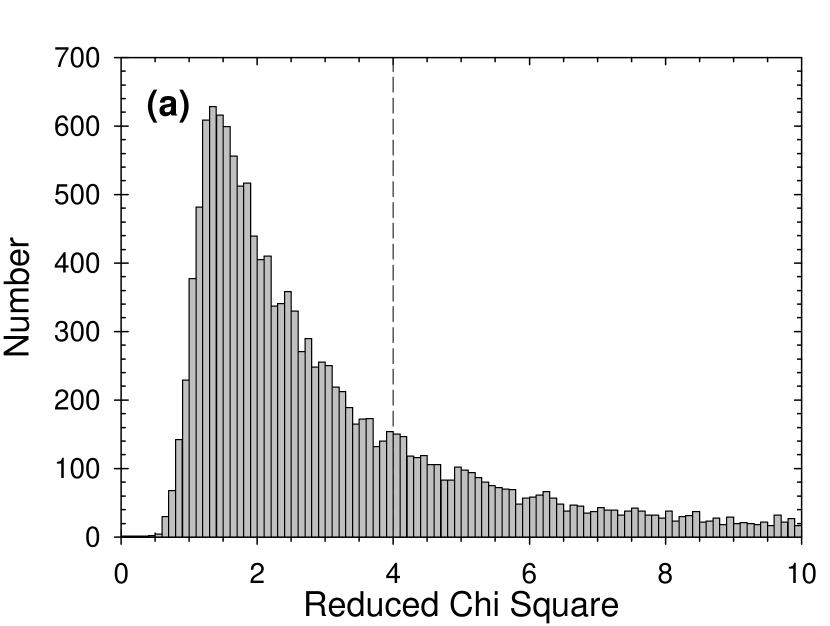
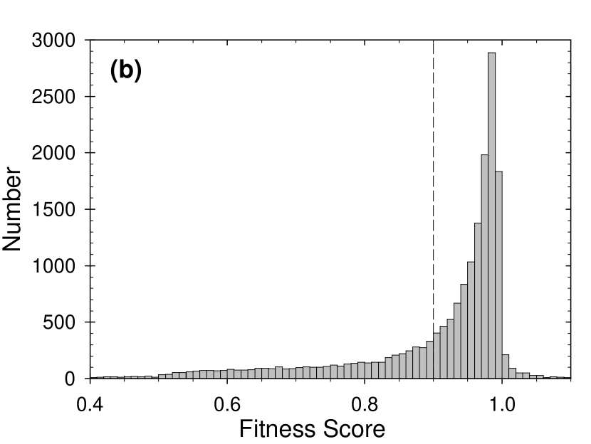
Figure 6: The distribution of: (a) reduced chi-square ($\chi_{\nu}^{2}$), and (b) fitness score results of the DEBiL model fits for OGLE II bulge (see appendix A). The vertical dashed lines mark the filtration thresholds used in our pipeline ($<4$ and $>0.9$ respectively). Both tests show a definite peak near 1, indicating that it is more likely that DEBiL will produce a “good” fit than a “bad” fit.

Most of the fits that reach step (6) can be considered successful (fig. 6). It is then up to the user to choose criteria for light curves that are of interest, and to define a threshold for the quality of the fits. In our pipeline we chose a very liberal quality threshold ($\chi_{\nu}^{2}<4$), so to allow through light curves with photometric uncertainties that are too small (a common occurrence), and to leave users with a large amount of flexibility in their further filtrations. We list the first 15 DEBiL fits that passed though step (6) in table 4. Figure 7 shows another sampling of models, with their corresponding phased light curves. The complete dataset of OGLE II bulge models, both plotted and in machine readable form, is available online.

Since the filter at step (6) may not be stringent enough for many application, we also provide our results after each of two further levels of filtration:

• Non-pulsating (fitness score $>0.9$; non-sinusoidal light curves): 8471

• Detached systems (both stars are within their Roche limit): 3170

For non-sinusoidal light curves, we require that the DEBiL fit have a smaller reduced chi square than the best-fit sinusoidal model. For the Roche limit calculation, we assumed an early main sequence mass-radius power law relation: $R\propto M^{0.652}\;$ (Gorda & Svechnikov, 1998) and set it in a third order approximation of the Roche radius (de Loore & Doom, 1992). The resulting approximations are:

$$R_{Roche,1}/a \simeq 0.37771+0.31054x+0.04324x^{2}+0.08208x^{3}$$ (4)

$$R_{Roche,2}/a \simeq \cases{0.37710-0.32684x-0.01882x^{2}-0.023812x^{3},&if x $\geq 0.65$\cr 0.37771-0.31054x+0.04324x^{2}-0.08208x^{3},&otherwise\cr}$$ (5)

Where: $x\equiv\log\left({R_{1}/R_{2}}\right)\;$, assuming: $R_{1}\geq R_{2}$.

In order to better interpret the data derived by the DEBiL pipeline, we combined it with color (V-I) and magnitude information (Udalski et al., 2002), as well as an extinction map of the galactic bulge (Sumi, 2004). Thus for each eclipsing system, we also have its extinction corrected combined I-band magnitude and V-I color. Since many of the stars in the bulge fields are not in the galactic bulge but rather in the foreground, it is likely they will be overcorrected, making them too blue and too bright. These stars can be seen in both the color-magnitude diagram (fig. 8) and in the color-density diagram (fig. 9). With this qualification in mind, the color-density diagram provides a distance independent tool for identifying star types. Because the measured values result from a combination of the two stars in the binary, the values aren’t expected to precisely match either one of the stars in a binary. Remarkably, using the max density measure instead of the mean density (appendix B) this problem seems to be considerably lessened.

5.1 Population Distributions

Due to the limitations of the OGLE observations, analysis and subsequent filtrations, there are a myriad of complex selection effects that need to be accounted for. For this reason, we hesitate to make any definite population statements in this paper, although there are a number of suggestive clusterings and trends that merit further scrutiny.

When considering the distribution of $r_{1,2}\equiv R_{1,2}/a$ for eclipsing binary systems, one would expect a comparably smooth distribution as determined by the binary star IMF, binary orbit dynamics and observational/detection selection effects. This distribution can be best seen in a radius-radius plot (fig. 10). This plot has a few features which merit discussion. One feature is that the number of systems rapidly dwindles as their radii become smaller. This should not be surprising as selection effects dominate the expected number of observed systems, for small radii (this point will be elaborated at the end of this subsection). A second, far more surprising feature, is the appearance of three clusterings: along the contact limit, around $\left(r_{1}=0.33,r_{2}=0.23\right)$ and around $\left(r_{1}=0.15,r_{2}=0.09\right)$. These three clusterings are most likely artificial, caused by two technical limitations which are discussed in §3.3. The first two clusterings were likely formed when many of the semidetached systems that populated the region between the clusterings, were swept into the contact limit, because their radii were overestimated. The third clustering, though less pronounced, seems to echo the structure of the second clustering, only with about half its radii. This hints at the possibility that the periods of some of these systems were doubled when they shouldn’t have been, probably because of an undetected eclipse. It is worth mentioning that both the second and third clusterings are centered at a significant distance from $r_{1}=r_{2}$, which is where the clusters would have been located, if $r_{1}$ and $r_{2}$ had been independent variables.

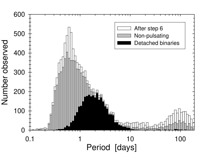
Figure 11: The period distribution of OGLE II bulge eclipsing binaries, following various stages of filtration.

Perhaps even more surprising is the period distribution (fig. 11). Using only the default filters of our pipeline, this distribution is bimodal, peaking at approximately 1 and 100 days, and with a desert around a 20-day period. To understand this phenomenon one should look at the scatter plots of figure 12. In this figure we can see that long period binaries (period $>20$ days) are significantly redder than average and have low eccentricities. This is possibly due to red giants, which cannot be in short period systems. This possibility is problematic since it contradicts the unimodal results of previous period distribution studies (Farinella et al., 1979; Antonello et al., 1980; Duquennoy & Mayor, 1991). In addition, figure 11 shows that with additional filtrations, the grouping of systems around the 100-day period is greatly reduced. All this leads us to conclude that the $\sim$100 day period peak is probably erroneous, created by a population contamination of pulsating stars, probably mostly semi-regulars, which can easily be confused with contact binaries. A similar phenomenon is seen in the spike in the number of system around a period of 0.6 days. This increase is probably also due to pulsating stars, only this time they are likely RR-Lyrae. They too were largely filtered out using the techniques described in the previous section.

Finally, we unraveled the geometric selection effects by weighting each eclipsing light curve by the inverse of the probability of observing it as eclipsing. For example, if with a random orientation there is a $1\%$ chance of a given binary systems being seen as eclipsing, we will give it a weight of 100. In this way we tabulated each observed occurrence as representing 100 such binary systems, the remaining of which exist but aren’t seen eclipsing and so are not included in our sample of variable stars. A binary system with a circular orbit (e = 0) will eclipse when its inclination angle (i) obeys: $\cos(i)<(R_{1}+R_{2})/a$. If the orbital orientations are randomly distributed, then the inclination angles are distributed as: $p(i)\propto\left|\sin(i)\right|$. Therefore, the probability that such a binary system will eclipse becomes:

$$p_{eclipse}(R_{1,2}/a,e=0)=\frac{R_{1}+R_{2}}{a}$$ (6)

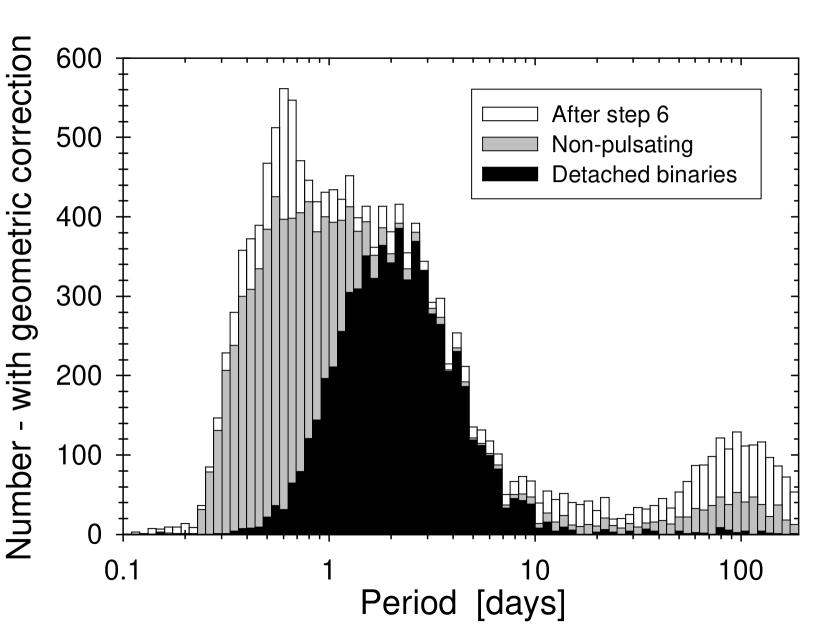
Figure 13: The period distribution of OGLE II bulge eclipsing binaries, following various stages of filtration, after correcting for their geometric selection effect.

The probability of eccentric systems (e $>0$) eclipsing is more difficult to calculate. We used a Monte-Carlo approach to calculate a 1000$\times$1000 $[(R_{1}+R_{2})/a,e]$ probability table, which was then used to interpolated the probability of each fitted light curve. When applying this correction for the geometric selection effect (fig. 13) we see that, as expected, it primarily effects the detached binaries. The period (P) distribution of detached systems, both before ($p_{eclipse}$) and after ($p_{all}$) the geometric correction are remarkably similar, and can both be well fit to a log-normal distribution:

$$p_{eclipse,all}(P)=\frac{1}{\sqrt{2\pi}\sigma P}\exp\left({-\frac{\ln^{2}(P/P_{0})}{2\sigma^{2}}}\right)$$ (7)

Before the geometric correction ($p_{eclipse}$) we get a fit of $P_{0}=1.83\pm 0.01$ days and $\sigma=0.593\pm 0.005$ ($r^{2}\simeq 0.9926$). After the correction ($p_{all}$) we get a fit of $P_{0}=2.06\pm 0.01$ days and $\sigma=0.621\pm 0.005$ ($r^{2}\simeq 0.9928$). Such log-normal distributions are generally indicative of many independent multiplicative processes taking place. Possibly, both in the formation of binary systems as well as in their observational/detection selection effects.

One should be very careful when using this method to calculate the total number of binaries. Simply comparing the number of binaries before and after the geometric correction will result in the conclusion that we are observing as eclipsing binaries about half of the total number of binaries. This fraction is biased high due to the fact that the OGLE II survey cannot detect long period eclipsing binaries.

5.2 Extreme Systems

In the previous subsection we considered the way large sets of eclipsing systems are distributed, now we will consider individual systems. As examples we chose to locate extreme binary systems, systems with a parameter well outside the normal range. For this to be done properly, we need to take great care in avoiding the pitfalls that arise from parameter estimation errors, both systematic and non-systematic. One pitfall is that some of the extreme systems may have large systematic errors since they will contain additional phenomena which the fitted model neglects. Another, perhaps more problematic pitfall, is that we will retrieve non-extreme systems with large errors that happen to shift the parameter in question beyond our filtering criterion threshold. Some examples of possible sources of large errors are inaccuracies in the correction for dust reddening (see the beginning of this section) and difficulties in the estimation of the argument of periastron, which directly affects the determination of binary’s orbital eccentricity (Etzel, 1991). Because of these pitfalls, we expect that the human eye will be required as the final decision maker for this task in the foreseeable future.

We present candidates of the most extreme eclipsing systems within the OGLE II bulge field dataset in five categories (table 5). We chose examples for which we were comparably confident, though we would need to follow them up with spectroscopic measurements to be certain of their designations.

In the case of the high density, low density and blue systems the measured value of the characteristic is a weighted mean of the two stars in the binary system. The weighting of the high and low density systems is described in appendix B. The weighting of the blue systems is determined, approximately, by the bolometric luminosity of each of the stars in the binary system.

6 Conclusions

We present a new multi-tiered method for systematically analyzing eclipsing binary systems within large-scale light curve surveys. In order to implement this method, we have developed the DEBiL fitter, a program designed to rapidly fit large number of light curves to a simplified detached eclipsing binary model. Using the results of DEBiL one can select small subsets of light curves for further follow-up. Applying this approach, we have analyzed 218699 light curves from the bulge fields of OGLE II, resulting in 10862 model fits. From these fits we identified unexpected patterns in their parameter distribution. These patterns are likely caused by selection effects and/or biases in the fitting program. The DEBiL model was designed to fit only fully detached systems, so users should use fits of semidetached and contact binary systems with caution. One can probably find a corrections for the parameters of these systems, though it is best to refit them using more complex models, which also take into account mutual reflection and tidal effects. Even so, the DEBiL fitted parameters will likely prove useful for quickly previewing large datasets, classification, fitting detached systems and providing an initial guess for more complex model fitters.

Appendix A Statistical Tests

A.1 Fitness Score

One of the problems with using the reduced chi-square test is that the light curve uncertainties may be systematically overestimated (underestimated), causing the reduced chi-square to be too small (large). An easy way to get around this problem is by comparing the reduced chi-square of the DEBiL model being considered, with the reduced chi-square of an alternative model. We used two simple alternative models:

- A constant, set to the average amplitude of the data.

- A smoothed spline, derived from a second order polynomial fit within a sliding kernel over the phased light curve.

The constant model should have a larger reduced chi-square than the best-fit model, while the spline model should usually have a smaller reduced chi-square. In a way similar to an F-test, we define the fitness score as:

$$\mbox{Fitness\ Score}\equiv\frac{\chi_{\nu}^{2}(\mbox{const})-\chi_{\nu}^{2}(\mbox{DEBiL})}{\chi_{\nu}^{2}(\mbox{const})-\chi_{\nu}^{2}(\mbox{spline})}$$ (A1)

This definition is useful since gross over- or underestimates of the uncertainties will largely cancel out. Light curves that reach step 6, will mostly have fitness scores between 0 and 1. If the reduced chi-square of the DEBiL model equals the constant model’s reduced chi-square, the fitness score will be 0, and if it equals the spline model’s reduced chi-square, the fitness score will be 1. The fact that most of the DEBiL models have fitness scores close to 1, and sometimes even surpassing it (fig. 6), provides a validation for the fitting algorithm used.

A.2 Scatter Score

This test quantifies the systematic scatter of data above or below the model, using the correlation between neighboring residuals. The purpose of this test is to quantify the quality of the model fit independently of the reduced chi-square test. While the reduced chi-square test considers the amplitude of the residuals, the scatter score considers their distribution. The scatter score is defined after folding the n data points into a phase curve:

$$\mbox{Scatter\ Score}\equiv\frac{\Delta X_{n}\cdot\Delta X_{1}+\sum\limits_{i=2}^{n}{\Delta X_{i-1}\cdot\Delta X_{i}}}{\sum\limits_{i=1}^{n}{\Delta X_{i}^{2}}}=\frac{\left\langle{\Delta X_{i-1}\cdot\Delta X_{i}}\right\rangle}{\left\langle{\Delta X_{i}^{2}}\right\rangle}$$ (A2)

Where: $\Delta X_{i}\equiv X_{i}(\mbox{data})-X_{i}(\mbox{model})$

The scatter score will always be between 1 and -1. A scores close to 1 occurs when all $\Delta X_{i}$ are approximately equal. In practice, this represent a severe systematic error, where the model is entirely above or entirely below the data. When there is no systematic error, the data are distributed randomly around the model, generating a scatter score approaching 0. Scores close to -1, although theoretically possible when $\Delta X_{i}\simeq-\Delta X_{i-1}$, can be considered unphysical in that they are unlikely to occur through systematic or non-systematic errors.

A.3 Waviness

This is a special case of the scatter score (see previous subsection). Here, we consider only data points in the light curve’s plateau (i.e. the region in the phased curve between the eclipsing dips, where both stars are fully exposed). The Waviness score is the scatter score of these data points around their median. The purpose of this test is to get a model-independent measure of irregularities in the binary brightness, out of eclipse. A large value may indicate such effects as stellar elongation, spots, or flares.

Appendix B Density Estimation

One of the most important criteria for selecting binaries for follow-up is its stellar density. Unfortunately, the parameters that can be extracted from the light curve fitting do not provide us with enough information for deducing the density of any one of the stars in the binary, but only a combined value. We define the mean density as the sum of the stars’ masses divided by the sum of their volumes:

$$\bar{\rho}\equiv\frac{M_{1}+M_{2}}{\left({4\pi/3}\right)\left({R_{1}^{3}+R_{2}^{3}}\right)}=\frac{3\pi}{GP^{2}\left({r_{1}^{3}+r_{2}^{3}}\right)}\simeq\frac{0.01893\,g\,{cm}^{-3}}{P_{day}^{2}\left({r_{1}^{3}+r_{2}^{3}}\right)}\simeq\frac{0.01344\,\rho_{\sun}}{P_{day}^{2}\left({r_{1}^{3}+r_{2}^{3}}\right)}$$ (B1)

Where: $r_{1,2}\equiv R_{1,2}/a$  and from Kepler’s law: $a^{3}=G\left({M_{1}+M_{2}}\right)\left(P/{2\pi}\right)^{2}$

It should be noted here that if the stars’ have very different sizes, their mean density will be dominated by the larger one, according to the weighted average:

$$\bar{\rho}=\frac{\left({r_{1}/r_{2}}\right)^{3}\rho_{1}+\rho_{2}}{\left({r_{1}/r_{2}}\right)^{3}+1}$$ (B2)

Similarly, assuming: $R_{1}\geq R_{2}$, the maximum possible density is:

$$\rho_{\max}\equiv\frac{M_{1}+M_{2}}{\left({4\pi/3}\right)R_{2}^{3}}=\bar{\rho}\left({1+\left({r_{1}/r_{2}}\right)^{3}}\right)\simeq\frac{0.01893\,g\,{cm}^{-3}}{P_{day}^{2}r_{2}^{3}}\simeq\frac{0.01344\,\rho_{\sun}}{P_{day}^{2}r_{2}^{3}}$$ (B3)

Adding the assumption that the more dense star of the binary is the less massive component, we can reduce the upper limit of its density to $\rho_{\max}/2$.

Table 1: FS Monocerotis (N = 249)

Parameters	Symbol	(Lacy et al., 2000)	DEBiL best fit	Relative error
Radius of primary (larger) star	$R_{1}/a$	0.2188 $\pm$ 0.0005	0.222 $\pm$ 0.003	1.3 %
Radius of secondary (smaller) star	$R_{2}/a$	0.173 $\pm$ 0.003	0.179 $\pm$ 0.006	3.5 %
Surface brightness ratio	$J_{s}$	0.903 $\pm$0.003	0.916 $\pm$ 0.05	1.5 %
Orbital inclination	i	87.48 $\pm$ 0.08	87.86 $\pm$ 0.015	0.4 %
Eccentricity	e	0.0 (fixed)	0.001 $\pm$ 0.01

Table 2: WW Camelopardalis (N = 5759)

Parameters	Symbol	(Lacy et al., 2002)	DEBiL best fit	Relative error
Radius of primary (larger) star	$R_{1}/a$	0.168 $\pm$ 0.0013	0.169 $\pm$ 0.018	0.5 %
Radius of secondary (smaller) star	$R_{2}/a$	0.159 $\pm$ 0.016	0.165 $\pm$ 0.014	3.4 %
Surface brightness ratio	$J_{s}$	0.950 $\pm$ 0.003	0.949 $\pm$ 0.08	0.1 %
Orbital inclination	i	88.29 $\pm$ 0.06	88.35 $\pm$ 0.03	0.1 %
Eccentricity	e	0.0099 $\pm$ 0.0007	0.01 $\pm$ 0.05

Table 3: BP Vulpeculae (N = 5236)

Parameters	Symbol	(Lacy et al., 2003)	DEBiL best fit	Relative error
Radius of primary (larger) star	$R_{1}/a$	0.1899 $\pm$ 0.0008	0.190 $\pm$ 0.006	0.1 %
Radius of secondary (smaller) star	$R_{2}/a$	0.161 $\pm$ 0.009	0.166 $\pm$ 0.009	3.1 %
Surface brightness ratio	$J_{s}$	0.624 $\pm$ 0.0013	0.614 $\pm$ 0.08	1.5 %
Orbital inclination	i	86.71 $\pm$ 0.09	86.50 $\pm$ 0.012	0.2 %
Eccentricity	e	0.0355 $\pm$ 0.0005	0.04 $\pm$ 0.03

Table 4: Selected parameters from the DEBiL dataset of eclipsing binary systems in the galactic bulge.

Field	Object	Period	e	$R_{1}/a$	$R_{2}/a$	$I_{1}$ [mag.]	$I_{2}$ [mag.]	$\sin(i)$	$t_{0}$	$\omega$ [deg.]	$\chi_{\nu}^{2}$	Corrected I [mag.]	Corrected V-I [mag.]
1	39	129.656	0.074	0.773	0.118	13.56	17.21	0.9208	0.665	256.0	1.13	12.81	1.93
1	45	0.55677	0.025	0.589	0.386	17.36	18.20	0.9979	0.724	271.4	1.06	16.21	-1000
1	53	2.52158	0.099	0.412	0.103	12.20	16.15	1.0000	0.418	91.4	3.07	11.38	0.18
1	108	1.53232	0.005	0.516	0.301	16.80	19.12	0.9143	0.497	254.1	0.93	15.84	0.48
1	112	0.35658	0.000	0.514	0.486	17.90	17.87	0.9763	0.429	40.6	1.56	16.36	0.65
1	155	0.96092	0.014	0.683	0.303	16.15	17.84	0.9203	0.199	294.5	1.12	15.10	0.45
1	183	0.57793	0.009	0.555	0.338	17.99	20.03	0.9828	0.055	56.4	1.29	17.14	0.41
1	201	0.67241	0.101	0.509	0.246	17.26	20.08	0.9971	0.473	264.3	0.87	16.44	0.32
1	202	4.51345	0.174	0.309	0.206	17.58	17.08	0.9968	0.035	270.9	2.68	15.82	0.64
1	215	0.48925	0.000	0.770	0.230	15.93	18.62	0.9212	0.870	150.5	1.54	15.06	0.20
1	221	0.45013	0.004	0.558	0.434	18.23	18.87	0.9332	0.107	100.7	0.92	16.92	0.58
1	227	122.879	0.007	0.700	0.294	16.69	18.39	1.0000	0.384	224.3	3.78	15.77	1.03
1	242	0.28142	0.003	0.521	0.476	18.56	18.67	1.0000	0.274	159.1	1.38	17.08	0.77
1	246	105.55	0.011	0.465	0.071	14.38	18.25	1.0000	0.280	192.1	3.68	13.57	1.19
1	257	2.37881	0.049	0.244	0.129	17.25	18.98	0.9855	0.510	87.5	0.88	16.33	0.66

Note. — This table is published in its entirety in the electronic edition of the Astrophysical Journal. A portion is shown here for guidance regarding its form and content.

Table 5: Extreme eclipsing binary system candidates

Category	Field	Object	Period	e	$R_{1}/a$	$R_{2}/a$	$I_{1}$ [mag.]	$I_{2}$ [mag.]	$\chi_{\nu}^{2}$	$\bar{\rho}$	$\rho_{\max}$	Corrected I [mag.]	Corrected V-I [mag.]
High density	21	5952	1.468	0.001	0.137	0.039	15.21	17.78	1.30	3.372	153.6	14.26	0.48
High density	23	1774	0.505	0.018	0.245	0.162	16.91	17.41	3.17	3.925	17.45	14.87	-1000
Low density	3	8264	151.026	0.023	0.487	0.228	17.39	18.95	2.53	0.000007	0.00007	15.46	1.33
Low density	21	2568	186.496	0.265	0.472	0.127	15.28	18.18	1.82	0.000005	0.00026	14.47	1.04
High eccentricity	2	547	2.419	0.231	0.211	0.077	12.12	14.66	1.89	0.330	7.049	11.47	-0.37
High eccentricity	38	4059	2.449	0.454	0.288	0.179	17.81	20.65	1.61	0.107	0.553	16.94	0.68
Blue	21	3797	2.653	0.003	0.193	0.104	12.33	14.35	3.03	0.322	2.373	11.48	-0.37
Blue	30	1778	6.442	0.084	0.089	0.028	12.81	15.53	2.39	0.627	21.37	11.81	-0.52
Short period	18	3424	0.179	0.119	0.670	0.211	16.73	19.28	2.10	1.895	62.905	15.53	0.13
Short period	46	797	0.198	0.072	0.444	0.426	16.67	16.60	2.80	2.913	6.208	14.87	1.36
Short period	49	538	0.228	0.008	0.728	0.264	16.09	18.35	1.07	0.904	19.929	15.03	0.31
Short period	42	2087	0.233	0.021	0.568	0.336	17.94	19.40	1.27	1.580	9.242	16.68	0.85

Figure 1: Diagram of a multi-tiered model-fitting pipeline.

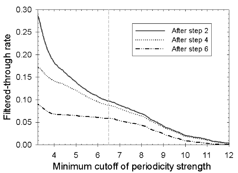
Figure 2: The pipeline filtration factions of the variables within bulge field 33 of OGLE II (N=4526), with varying periodicity strength cutoffs. The vertical dashed line indicates the chosen cutoff for our pipeline ($>6.5$).
[See http://cfa-www.harvard.edu/$\sim$jdevor/DEBiL.html for a high-resolution version of this figure]

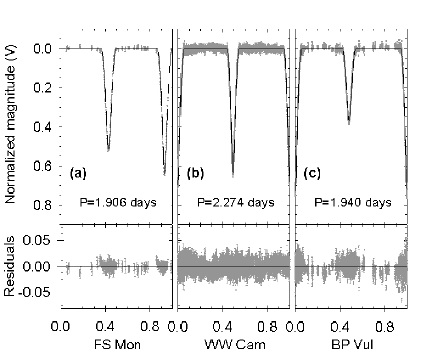
Figure 5: The phased light curves with the DEBiL model best fit (solid line) and its residuals, for the eclipsing binary systems: (a) FS Monocerotis; (b) WW Camelopardalis; (c) BP Vulpeculae.
[See http://cfa-www.harvard.edu/$\sim$jdevor/DEBiL.html for a high-resolution version of this figure]

Figure 7: Selected examples of OGLE II bulge field light curves, with their DEBiL fits.

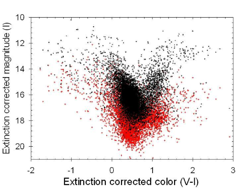
Figure 8: The color-magnitude diagram of both the primary (circles) and secondary (crosses) stars of the DEBiL models. The color of each star is the combined color of the binary, from (Udalski et al., 2002).
[See http://cfa-www.harvard.edu/$\sim$jdevor/DEBiL.html for a high-resolution version of this figure]

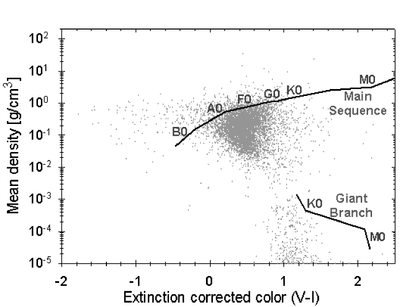
Figure 9: Color-density diagram of DEBiL models. The solid lines trace the main sequence stars and giants (Cox, 2000). Notice the strong observational selection bias for main sequence F-type and G-type stars in the OGLE II bulge fields.
[See http://cfa-www.harvard.edu/$\sim$jdevor/DEBiL.html for a high-resolution version of this figure]

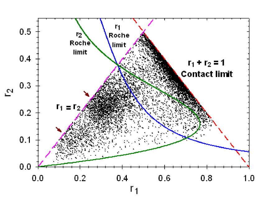
Figure 10: Radius-radius plot. The dashed lines mark the outer limit of the data. The left side is bounded by the fact that by definition: $r_{1}\geq r_{2}$ , while the right side is bounded by the physical contact limit of the stars. The two arrows mark anomalous clusterings. The two solid curves approximate the location where the primary and secondary stars reach their respective Roche limit (eq. 4 & 5). Systems between the two solid curves are semidetached, systems to their left are detached, and systems to their right are contact or overcontact systems.
[See http://cfa-www.harvard.edu/$\sim$jdevor/DEBiL.html for a high-resolution version of this figure]

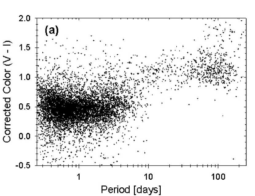
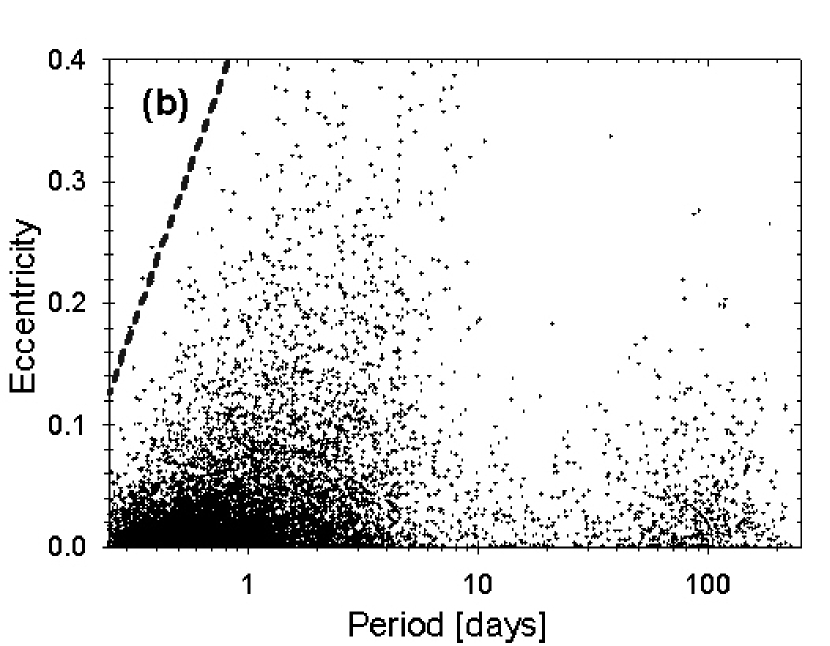
Figure 12: (a) Color-period plot and (b) eccentricity-period plot. The upper limit on the eccentricities of short period binaries (dashed line) is probably due to tidal circularization.
[See http://cfa-www.harvard.edu/$\sim$jdevor/DEBiL.html for a high-resolution version of these figures]

References

- Akerlof et al. (2000) Akerlof, C., et al. 2000, AJ, 119, 1901
- Alard & Guibert (1997) Alard, C. & Guibert, J. 1997, A&A, 326, 1
- Alard & Lupton (1998) Alard, C. & Lupton, R. H. 1998, ApJ, 503, 325
- Alcock et al. (1998) Alcock, C., et al. 1998, ApJ, 492, 190
- Alonso et al. (2004) Alonso, R., et al. 2004, ApJ, 613, L153
- Antonello et al. (1980) Antonello, E., Farinella, P., Guerrero, G., Mantegazza, L., & Paolicchi, P. 1980, Ap&SS, 72, 359
- Bakos et al. (2004) Bakos, G., Noyes, R. W., Kovács, G., Stanek, K. Z., Sasselov, D. D., & Domsa, I. 2004, PASP, 116, 266
- Beaulieu et al. (1995) Beaulieu, J. P., et al. 1995, A&A, 299, 168
- Charbonneau (1995) Charbonneau, P. 1995, ApJS, 101, 309
- Claret (2003) Claret, A. 2003, A&A, 401, 657
- Cox (2000) Cox, A. N. 2000, Allen’s astrophysical quantities, (4th ed.; New York: AIP Press; Springer)
- Crotts (1992) Crotts, A. P. S. 1992, ApJ, 399, L43
- Danby (1964) Danby, J. M. A. 1964, Fundamentals of Celestial Mechanics (New York: Macmillan)
- de Loore & Doom (1992) de Loore, C. & Doom, C. 1992, Structure and Evolution of Single and Binary Stars, Astrophysics and Space Science Library, Vol. 179 (Dordrecht: Kluwer)
- Duquennoy & Mayor (1991) Duquennoy, A. & Mayor, M. 1991, A&A, 248, 485
- Etzel (1981) Etzel, P. B. 1981, in Photometric and Spectroscopic Binary Systems (Dordrecht: Reidel)
- Etzel (1991) Etzel, P. B. 1991, International Amateur-Professional Photoelectric Photometry Communications, 45, 25
- Farinella et al. (1979) Farinella, P., Luzny, F., Mantegazza, L., & Paolicchi, P. 1979, ApJ, 234, 973
- Gorda & Svechnikov (1998) Gorda, S. Y. & Svechnikov, M. A. 1998, Astronomy Reports, 42, 793
- Holland (1992) Holland, J. H. 1992, Adaptation in Natural and Artificial Systems (2nd ed.; Cambridge: MIT Press)
- Kaiser et al. (2002) Kaiser, N., et al. 2002, Proc. SPIE, 4836, 154
- Kaluzny et al. (1998) Kaluzny, J., Stanek, K. Z., Krockenberger, M., Sasselov, D. D., Tonry, J. L., & Mateo, M. 1998, AJ, 115, 1016
- Kirkpatrick et al. (1983) Kirkpatrick, S., Gelatt, C. D., & Vecchi, M. P. 1983, Science, 220, 671
- Lacy et al. (2000) Lacy, C. H. S., Torres, G., Claret, A., Stefanik, R. P., Latham, D. W., & Sabby, J. A. 2000, AJ, 119, 1389
- Lacy et al. (2002) Lacy, C. H. S., Torres, G., Claret, A., & Sabby, J. A. 2002, AJ, 123, 1013
- Lacy et al. (2003) Lacy, C. H. S., Torres, G., Claret, A., & Sabby, J. A. 2003, AJ, 126, 1905
- Maceroni & Rucinski (1997) Maceroni, C., & Rucinski, S. M. 1997, PASP, 109, 782
- Maceroni & Montalbán (2004) Maceroni, C., & Montalbán, J. 2004, A&A, 426, 577
- Mallén-Ornelas et al. (2003) Mallén-Ornelas, G., Seager, S., Yee, H. K. C., Minniti, D., Gladders, M. D., Mallén-Fullerton, G. M., & Brown, T. M. 2003, ApJ, 582, 1123
- Nelder (1965) Nelder, J. A., & Mead 1965, R., Computer Journal, 7, 308
- Nelson & Davis (1972) Nelson, B. & Davis, W. D. 1972, ApJ, 174, 617
- Otten & van Ginneken (1989) Otten, R. H. J. M., & van Ginneken, L.P.P.P. 1989, The Annealing Algorithm (Dordrecht: Kluwer)
- Paczynski (1986) Paczynski, B. 1986, ApJ, 304, 1
- Paczynski (1996) Paczynski, B. 1996, in The Extragalactic Distance Scale, ed. M. Livio, M. Donahue, & N. Panagia (Cambridge: Cambridge Univ. Press), 273
- Phillips & Davis (1995) Phillips, A. C., & Davis, L. E. 1995, ASP Conf. Ser. 77, Astronomical Data Analysis and Software System IV, ed. R. A. Shaw et al. (San Francisco: ASP), 297
- Popper (1981) Popper, D. M. 1981, Revista Mexicana de Astronomia y Astrofisica, 6, 99
- Popper & Etzel (1981) Popper, D. M. & Etzel, P. B. 1981, AJ, 86, 102
- Press et al. (1992) Press, W. H., Teukolsky, S. A., Vetterling, W. T., & Flannery, B. P. 1992, (2nd ed.; Cambridge: University Press)
- Schwarzenberg-Czerny (1989) Schwarzenberg-Czerny, A. 1989, MNRAS, 241, 153
- Schwarzenberg-Czerny (1996) Schwarzenberg-Czerny, A. 1996, ApJ, 460, L107
- Seager & Mallén-Ornelas (2003) Seager, S. & Mallén-Ornelas, G. 2003, ApJ, 585, 1038
- Sumi (2004) Sumi, T. 2004, MNRAS, 349, 193
- Szalay & Gray (2001) Szalay, A. & Gray, J. 2001, Science, 293, 2037
- Tyson (2002) Tyson, J. A. 2002, Proc. SPIE, 4836, 10
- Udalski et al. (1994) Udalski, A., et al. 1994, Acta Astronomica, 44, 165
- Udalski et al. (1997) Udalski, A., Kubiak, M., & Szymanski, M. 1997, Acta Astronomica, 47, 319
- Udalski et al. (2002) Udalski, A., et al. 2002, Acta Astronomica, 52, 217
- Vanderbilt & Louie (1983) Vanderbilt, D., & Louie, S. G. 1983, Journal of Comp. Phys., 56, 259
- Wilson & Devinney (1971) Wilson, R. E. & Devinney, E. J. 1971, ApJ, 166, 605
- Wilson (1979) Wilson, R. E. 1979, ApJ, 234, 1054
- Wilson (1994) Wilson, R. E. 1994, PASP, 106, 921
- Wozniak et al. (2002) Wozniak, P. R., Udalski, A., Szymanski, M., Kubiak, M., Pietrzynski, G., Soszynski, I., & Zebrun, K. 2002, Acta Astronomica, 52, 129
- Wyithe & Wilson (2001) Wyithe, J. S. B. & Wilson, R. E. 2001, ApJ, 559, 260
- Wyithe & Wilson (2002) Wyithe, J. S. B. & Wilson, R. E. 2002, ApJ, 571, 293