Breaking scale invariance
from a singular inflaton potential

Abstract

In this paper we break the scale invariance of the primordial power spectrum of curvature perturbations of inflation. Introducing a singular behaviour due to spontaneous symmetry breaking in the inflaton potential, we obtain fully analytic expressions of scale dependent oscillation and a modulation in power on small scale in the primordial spectrum. And we give the associated cosmic microwave background and matter power spectra which we can observe now and discuss the signature of the scale dependence. We also address the possibility of whether some inflationary model with featured potential might mimic the predictions of the scale invariant power spectrum. We present some examples which illustrate such degeneracies.

KAIST-TH/2005-06

1 Introduction

Inflation [1], an epoch of accelerated expansion in the earliest history of the universe, is believed to be able to solve many problems of standard big bang cosmology, such as homogeneity, isotropy and flatness of the universe we observe now. Among them, one of the most important for current and future observations is the generation of density perturbations from quantum fluctuations in the inflaton field [2, 3]. Once those perturbations develop, they become the seeds of the fluctuations in the otherwise homogeneous and isotropic cosmic microwave background (CMB) and matter distribution in the subsequent evolution of the universe.

For inflationary models driven by a scalar field slowly rolling down the potential, the density perturbations produced during inflation are generally expected to be nearly scale invariant; that is, the power spectrum of those primordial perturbations are predicted to be $\mathcal{P}(k)\propto k^{n-1}$ with $n\sim 1$, where the deviation from $n=1$ depends on the detailed dynamics of the inflaton. In this ‘slow-roll’ approximation we have the spectral index $n$ as a function of the potential and its derivatives, or slow-roll parameters, which distinguish different inflationary models. They are required to be small in common to maintain the scale invariance, which is as stated above, the consequence of the inflaton field slowly rolling down the smooth potential. Certainly, recent observations put strong bound on $n$; it must be close to 1 [4].

However, the scale invariance of $\mathcal{P}(k)$ is not directly constrained by experiments but assumed. The spectra we can observe are the CMB and matter power spectra, which are believed to have been generated from the common $\mathcal{P}(k)$, multiplied by some transfer functions describing the complicated physics of the evolution. We believe the scale invariance since the observations on large scales, where the linearity preserves the basic properties of primordial fluctuations, fit fairly with $\mathcal{P}(k)$ with $n\sim 1$, not since we actually observe the very scale invariant $\mathcal{P}(k)$ directly, nor since it is the only theoretical possibility. As mentioned above, when the inflaton rolls down the smooth potential slowly, the power spectrum becomes very close to the flat one, with $n\sim 1$. But the slow-roll approximation does not encompass all the possibilities of inflation. For example, even the potential exhibits singular behaviours and the inflaton field does not slowly roll down the potential so that the standard slow-roll scheme is not applicable [5, 6], still it is possible to keep inflation going on. In this case, generally we obtain a scale dependent primordial power spectrum $\mathcal{P}(k)$ [7, 8, 9, 10, 11, 12], possibly leading to a detectable discrepancy between the standard cosmological model and observations such as the dearth of halo substructure [9] and the suppression of the low multipoles in the CMB anisotropy [13].

As the origin of such singular behaviour, we can think of the general situation that inflaton field $\phi$ is coupled to other scalar fields. During inflation, those scalar fields may undergo spontaneous symmetry breaking, so that they acquire some nonzero vacuum expectation values. Provided that the symmetry breaking is rapid, the coupled scalar fields would result in a non-smooth behaviour in the inflaton potential [12, 14]. For example, consider a simple toy model where the effective potential contains quadratic terms of scalar fields $\phi$ and $\varphi$ as

$$V(\phi,\varphi)=V_{0}-\mu^{3}\phi-m_{\varphi\phi}^{2}\varphi\phi\,.$$ (1)

When $\varphi$ acquires vacuum expectation value $v$, we can see that around the moment of symmetry breaking the ‘slope’ of the potential $V(\phi)$ changes. For a more realistic example, we move to another simple model where the effective potential of two scalar fields $\phi$ and $\varphi$ is given as [7]

$$V(\phi,\varphi)=V_{0}-\frac{1}{2}m_{\phi}^{2}\phi^{2}-\frac{1}{2}g^{2}\phi^{2}\varphi^{2}\,.$$ (2)

Now assume that by spontaneous symmetry breaking the field $\varphi$ acquires a nonzero vacuum expectation value $\langle\varphi\rangle=v$ when $\phi$ becomes greater than some critical value $\phi_{c}$; then the mass of $\phi$ is modified. Then the corresponding potential is

$$V(\phi)=V_{0}-\frac{1}{2}\left(m_{\phi}^{2}+g^{2}v^{2}\right)\phi^{2}\,.$$ (3)

Clearly we see that there is a downward behaviour at the moment of symmetry breaking.

Thus, it is meaningful and interesting to open the possibility of non-smooth, featured potential and to investigate the resulting power spectrum on both theoretical and observational grounds. Here we consider some inflaton potentials with singular, non-smooth behaviours and calculate the fully analytic results for the primordial power spectrum $\mathcal{P}(k)$ of the curvature perturbations. Using those $\mathcal{P}(k)$, we present the subsequent CMB and matter power spectra relevant for observations, and discuss the viability of such featured potentials. The possibility of broken scale invariance has been studied several times numerically [7, 9, 10, 11], but here we obtain fully analytic results for $\mathcal{P}(k)$ as far as we can.

This paper is organised as follows. First, in Section 2 we review the generalised slow-roll formalism, which we will use in the following Section 3 to derive the primordial power spectrum of curvature perturbations for potentials with feature such as slope change and step. In Section 4 we describe the CMB and matter power spectra associated with $\mathcal{P}(k)$ of the previous section, and discuss the possibility of degeneracy surviving the current observational constraints. In Section 5 we summarise the results and conclude. Throughout the paper we set $c=\hbar=8\pi G=1$.

2 General Slow-Roll Formalism

When we deal with some inflaton potential which is not smooth, it is not guaranteed that the slow-roll parameters,

$$\epsilon\equiv-\frac{\dot{H}}{H^{2}}=-\frac{d\ln H}{d\ln a}\hskip 28.45274pt\mbox{and}\hskip 28.45274pt\delta_{1}\equiv\frac{\ddot{\phi}}{H\dot{\phi}}=\frac{d\ln\dot{\phi}}{d\ln a}\,,$$ (4)

are approximately constants. Therefore, naively applying the standard slow-roll approximation, where it is additionally assumed that $\epsilon$ and $\delta_{1}$ are both slowly varying, does not work. Instead we must use some other scheme which encompasses the cases where the standard slow-roll picture is not applicable to solve the situation analytically; we adopt the general slow-roll picture. In this section, we briefly review the Green’s function method [16] and the general slow-roll approximation discussed in [5, 6]. Then we write the power spectrum of the density perturbations which we will use in the next section.

The scalar perturbation to the homogeneous, isotropic background metric is generally given by [3]

$$ds^{2}=a^{2}(\eta)\left\{(1+2A)d\eta^{2}-2\partial_{i}Bdx^{i}d\eta-[(1-2\psi)\delta_{ij}+2\partial_{i}\partial_{j}E]dx^{i}dx^{j}\right\}\,,$$ (5)

and we define

$$\varphi=a\left(\delta\phi+\frac{\dot{\phi}}{H}\psi\right)\hskip 28.45274pt\mbox{and}\hskip 28.45274ptz=\frac{a\dot{\phi}}{H}\,,$$ (6)

then the intrinsic curvature perturbation of the comoving hypersurfaces is given by

$$\mathcal{R}_{\mathrm{c}}=\frac{\varphi}{z}\,,$$ (7)

and the equation of motion for the Fourier component of $\varphi$ is given by

$$\frac{d^{2}\varphi_{k}}{d\eta^{2}}+\left(k^{2}-\frac{1}{z}\frac{d^{2}z}{d\eta^{2}}\right)\varphi_{k}=0\,,$$ (8)

where $\varphi_{k}$ satisfies the boundary conditions

$$\varphi_{k}\longrightarrow\left\{\begin{array}[]{ccc}\frac{1}{\sqrt{2k}\,}e^{-ik\eta}&\mbox{as}&-k\eta\rightarrow\infty\\ A_{k}z&\mbox{as}&-k\eta\rightarrow 0\,.\end{array}\right.$$ (9)

Now, writing $y\equiv\sqrt{2k}\,\varphi_{k}$, $x\equiv-k\eta$ and

$$f(\ln x)\equiv\frac{2\pi xz}{k}=\frac{2\pi}{H}\frac{ax\dot{\phi}}{k}\,,$$ (10)

Eq. (8) becomes

$$\frac{d^{2}y}{dx^{2}}+\left(1-\frac{2}{x^{2}}\right)y=\frac{g(x)}{x^{2}}y\,,$$ (11)

where $g\equiv(f^{\prime\prime}-3f^{\prime})/f$ and $f^{\prime}\equiv df/d\ln x$. Using Green’s function method, we can present the solution of Eq. (11) as an integral equation

$$y(x) = y_{0}(x)+\frac{i}{2}\int_{x}^{\infty}\frac{du}{u^{2}}\,g(u)\left[y_{0}^{*}(u)\,y_{0}(x)-y_{0}^{*}(x)\,y_{0}(u)\right]y(u)$$ (12)

$$\equiv y_{0}(x)+L(x,u)\,y(u)\,,$$

where

$$y_{0}(x)=\left(1+\frac{i}{x}\right)e^{ix}$$ (13)

is the homogeneous solution with desired asymptotic behaviour.

The power spectrum for the curvature perturbation $\mathcal{P}(k)$ is defined by

$$\frac{2\pi^{2}}{k^{3}}\,\mathcal{P}(k)\,\delta^{(3)}(\mathbf{k-l})=\langle\mathcal{R}_{\mathrm{c}}(\mathbf{k})\,{\mathcal{R}_{\mathrm{c}}}^{\dagger}(\mathbf{l})\rangle\,,$$ (14)

which, using the above results, we can write conveniently as

$$\mathcal{P}(k)=\lim_{x\rightarrow 0}\left|\frac{xy}{f}\right|^{2}\,.$$ (15)

Here, we only assume that $y(x)$ is given approximately by the scale invariant $y_{0}(x)$, or equivalently that $g$ is small. It is very important to note that this is the only assumption we make as required by observations. Then, since we are interested in the second order corrections, we iterate Eq. (12) twice, i.e.,

$$y(x)\simeq y_{0}(x)+L(x,u)\,y_{0}(u)+L(x,u)\,L(u,v)\,y_{0}(v)\,.$$ (16)

Substituting into Eq. (15), and skipping over calculations, we can rewrite the power spectrum as [6]

$$\ln\mathcal{P}(k) = \ln\left(\frac{1}{f_{\star}^{2}}\right)+\frac{2}{3}\frac{f^{\prime}_{\star}}{f_{\star}}+\frac{1}{9}\left(\frac{f^{\prime}_{\star}}{f_{\star}}\right)^{2}+\frac{2}{3}\int_{0}^{\infty}\frac{du}{u}\,W_{\theta}(x_{\star},u)\,g(u)+\frac{2}{9}\left[\int_{0}^{\infty}\frac{du}{u}\,X(u)\,g(u)\right]^{2}$$ (18)

$$\mbox{}-\frac{2}{3}\int_{0}^{\infty}\frac{du}{u}\,X(u)\,g(u)\int_{u}^{\infty}\frac{dv}{v^{2}}\,g(v)-\frac{2}{3}\int_{0}^{\infty}\frac{du}{u}\,X_{\theta}(x_{\star},u)\,g(u)\int_{u}^{\infty}\frac{dv}{v^{4}}\,g(v)$$

$$= \ln\left(\frac{1}{f_{\star}^{2}}\right)-2\int_{0}^{\infty}\frac{du}{u}\,w_{\theta}(x_{\star},u)\,\frac{f^{\prime}}{f}+2\left[\int_{0}^{\infty}\frac{du}{u}\,\chi(u)\,\frac{f^{\prime}}{f}\right]^{2}$$

$$\mbox{}-4\int_{0}^{\infty}\frac{du}{u}\,\chi(u)\,\frac{f^{\prime}}{f}\int_{u}^{\infty}\frac{dv}{v^{2}}\,\frac{f^{\prime}}{f}$$

where the window functions are given as

$$W(x) = \frac{3\sin(2x)}{2x^{3}}-\frac{3\cos(2x)}{x^{2}}-\frac{3\sin(2x)}{2x}\,,$$

$$X(x) = -\frac{3\cos(2x)}{2x^{3}}-\frac{3\sin(2x)}{x^{2}}+\frac{3\cos(2x)}{2x}+\frac{3(1+x^{2})}{2x^{3}}\,,$$

$$W_{\theta}(x_{\star},x) = W(x)-\theta(x_{\star}-x)\,,$$

$$X_{\theta}(x_{\star},x) = X(x)-\frac{x^{3}}{3}\,\theta(x_{\star}-x)\,,$$

$$w(x) = W(x)+\frac{x}{3}W^{\prime}(x)\,,$$

$$\chi(x) = X(x)+\frac{x}{3}X^{\prime}(x)\,,$$

$$w_{\theta}(x_{\star},x) = w(x)-\theta(x_{\star}-x)\,,$$ (19)

and the subscript $\star$ means some convenient point of evaluation around horizon crossing.

3 $\mathcal{P}(k)$ from non-smooth inflaton potential

Now, using Eqs. (18) and (18) for the power spectrum derived in the previous section, we consider some curvature power spectra $\mathcal{P}(k)$ for the models of inflation arising from the potentials with some singular behaviours.

Before we start this section, let us remind that we would like to consider the cases where we cannot apply the slow-roll conditions usually assumed; $\dot{\phi}$ or $\ddot{\phi}$ is changing drastically, and the features should be extremely singular, or very sharp. Then, the somewhat ad hoc features we are going to discuss here are good enough approximations, and they are our starting point. Also note that since mild enough features are highly dependent on the detail of specific models under consideration, it is not easy to extract other than qualitative behaviour. But sharp cases are universal; as we will see, we need only a single or a couple of parameters to characterise the feature, and we acquire complete control of that singularity.

3.1 Linear potential with a slope change

This kind of model has been investigated several times [6, 8], so we skip straightforward calculations and just present the situation and the result. We consider an inflaton $\phi$ rolling down a linear potential with slope changing from $-A$ to $-A-\Delta A$ at $\phi=\phi_{0}$. We can write the potential as

$$V(\phi)=V_{0}\left\{1-\left[A+\theta(\phi-\phi_{0})\,\Delta A\right]\left(\phi-\phi_{0}\right)\right\}\,.$$ (20)

Assuming $|A|\ll 1$ so that $3H^{2}=V_{0}$ and $x=k/(aH)$, and solving the equation of motion for $\phi$, we obtain

$$\frac{d\phi}{dN}=A+\theta(N-N_{0})\,\Delta A\left[1-e^{-3(N-N_{0})}\right]\,,$$ (21)

where $N=\int H\,dt$ and $\phi(N_{0})=\phi_{0}$. Then if $|\Delta A/A|\ll 1$ so that the approximate scale invariance of the spectrum is maintained, we have

$$\frac{V^{\prime\prime}}{V}=-\frac{1}{3}g=-\Delta A\,\delta(\phi-\phi_{0})=-\frac{\Delta A}{A}\,\delta(N-N_{0})\,,$$ (22)

where $x_{0}=k/(aH)_{0}=k/k_{0}$. Substituting into Eq. (18) and performing the integration, we find the power spectrum as [6]

$$\ln\mathcal{P} = \ln\left(\frac{V_{0}}{12\pi^{2}A^{2}}\right)+2\left(\frac{\Delta A}{A}\right)\left[W(x_{0})-1\right]$$ (23)

$$+2\left(\frac{\Delta A}{A}\right)^{2}\left\{X(x_{0})\left[X(x_{0})-\frac{3(1+x_{0}^{2})}{2x_{0}^{3}}\right]+\frac{1}{2}\right\}\,.$$

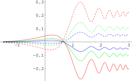
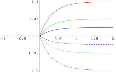
The spectrum $\ln\mathcal{P}$ is plotted in the left panel of Figure 1. In addition to the constant leading term $\ln\left[V_{0}/(12\pi^{2}A^{2})\right]$, the most important change from the scale invariant $\mathcal{P}(k)$ is that there is a modulation in power, a suppression (an enhancement), after the slope change when the change is positive (negative). Also we obtain an diminishing oscillation after the slope change. Another noteworthy point is the behaviour of $d\phi/dN$ shown in the right panel of Figure 1. When $\Delta A<0$, i.e., the slope becomes flatter, $d\phi/dN$ gets smaller than its value at horizon crossing. Then, the perturbations on the scales smaller than the very scale of slope change experience enhancement after they go outside the horizon; as shown in the left panel of Figure 1, $\mathcal{P}(k)$ is rising across $\ln x_{0}=0$. This agrees precisely with Ref. [10].

Figure 1: (Left) plot of $\ln\mathcal{P}$ versus $\ln x_{0}$, Eq. (23), and (right) $d\phi/dN$ versus $N$, Eq. (21), where $A$ is normalised to 1. Solid lines correspond to $\Delta A/A>0$ and dashed lines to $\Delta A/A<0$. $\left|\Delta A/A\right|$ are set to 0.025, 0.05 and 0.1 from the innermost line. As expected, the modulation in power becomes stronger as the slope change is steeper.

3.2 Linear potential with a sharp downward step

Now, we consider the situation where the potential is linear with slope $-A$, and there is a sharp downward step of size $aV_{0}$ at $\phi_{s}$. The potential can be written as

$$V(\phi)=V_{0}\left[1-A(\phi-\phi_{s})-a\theta(\phi-\phi_{s})\right]\,,$$ (24)

where we assume that $A\ll 1$, $a\ll 1$ and $a\ll A^{2}$ so that inflation is not suspended in spite of the existence of the step and $3H^{2}=V_{0}$.

In this case, we are unable to proceed as before because of the singularity in the slope, i.e., we have a delta function for $V^{\prime}(\phi)$. Rather, we use the relation $f^{\prime}/f=-\phi^{\prime\prime}/\phi^{\prime}$, where $\phi^{\prime}=d\phi/dN$, and Eq. (18). The equation of motion for $\phi$ is

$$\phi^{\prime\prime}+3\phi^{\prime}-3A=3a\delta(\phi-\phi_{s})\,,$$ (25)

where $\phi_{s}=\phi(N_{s})$, so we have two solutions

$$\phi(N)=\left\{\begin{array}[]{lll}A(N-N_{s})&\equiv\phi_{1}(N),&\mbox{before the step}\\ A\left[N-e^{-3(N-N_{s})}N_{s}\right]&\equiv\phi_{2}(N),&\mbox{after the step}\end{array}\right.$$ (26)

where we set $\phi_{s}=0$. Then, we can write the general solution of $\phi(N)$ as

$$\phi(N)=\phi_{1}(N)-\frac{B}{3N_{s}}\left[\phi_{1}(N)-\phi_{2}(N)\right]\theta(N-N_{s})$$ (27)

where we introduced a new parameter $B\equiv aV_{0}/A^{2}\ll 1$, which corresponds to the magnitude of the step. Then, we can write

$$\frac{f^{\prime}}{f} = -\frac{\phi^{\prime\prime}}{\phi^{\prime}}$$

$$= -B\left[\delta(x-x_{s})-3\theta(x_{s}-x)\right]\left(\frac{x}{x_{s}}\right)^{3}+B^{2}\left[\theta(x_{s}-x)\delta(x-x_{s})-3\theta(x_{s}-x)\right]\left(\frac{x}{x_{s}}\right)^{6}\,,$$

so from Eq. (18) we obtain the power spectrum as

$$\ln\mathcal{P} = \ln\left(\frac{V_{0}}{12\pi^{2}A^{2}}\right)+B\left[-\frac{3\sin(2x_{s})}{x_{s}^{3}}+\frac{6\cos(2x_{s})}{x_{s}^{2}}+\frac{5\sin(2x_{s})}{x_{s}}-2\cos(2x_{s})\right]$$ (29)

$$+B^{2}\left[1+\frac{9}{4x_{s}^{6}}+\frac{3}{2x_{s}^{4}}+\frac{1}{4x_{s}^{2}}-\frac{9\cos(2x_{s})}{2x_{s}^{6}}-\frac{9\sin(2x_{s})}{x_{s}^{5}}+\frac{6\cos(2x_{s})}{x_{s}^{4}}+\frac{5\cos(2x_{s})}{2x_{s}^{2}}\right.$$

$$\hskip 42.67912pt+\cos(2x_{s})+\frac{9\cos(4x_{s})}{4x_{s}^{6}}+\frac{9\sin(4x_{s})}{x_{s}^{5}}-\frac{33\cos(4x_{s})}{2x_{s}^{4}}-\frac{18\sin(4x_{s})}{x_{s}^{3}}$$

$$\hskip 42.67912pt\left.+\frac{49\cos(4x_{s})}{4x_{s}^{2}}+\frac{5\sin(4x_{s})}{x_{s}}-\cos(4x_{s})\right]\,.$$

Interestingly, now we have a scale dependent oscillatory behaviour in the spectrum. The spectra, Eq. (29), with a few different values of $B$ are shown in Figure 2. Across the step, $\ln(k/k_{s})=0$, there is an oscillation the amplitude of which depends on $B$. There are two important differences from the case of a slope change. One thing is that there is no power modulation in the small scale on average; the power spectrum oscillates around the value without the step. The other important point is that the oscillation does not diminish, and survives down to the small scales. These two points become distinct compared with the case of slope change in the CMB and matter power spectra which shall be discussed in the following section.

Figure 2: (Dashed) plot of $\ln\mathcal{P}$ versus $\ln x_{s}$ for a sharp step, Eq. (29), and (solid) an arctangent step, Eq. (44). The parameters for the arctangent step are set to $a=0.001$, $b=0.02\times(0.8)^{n}$ $A=(0.8)^{3n+1}$ where $n=2,3$ and 7/2 from the innermost line. These numbers are chosen to roughly match the first few peaks of the sharp step cases with $B=0.1,0.5$ and 1.0.

3.3 Linear potential with 2 successive slope changes

Here, we consider a linear potential with two successive slope changes, from $-A$ to $-A-\Delta A$ at $\phi_{1}=\phi(N_{1})$, and then back to $-A$ at $\phi_{2}=\phi(N_{2})$. Then, we can write the potential as

$$V(\phi)=V_{0}\left\{1-A(\phi-\phi_{1})-\Delta A\left[\theta(\phi-\phi_{1})(\phi-\phi_{1})-\theta(\phi-\phi_{2})(\phi-\phi_{2})\right]\right\}\,.$$ (30)

As before, assuming $|A|\ll 1$, we have

$$\frac{V^{\prime\prime}}{V}=-\frac{\Delta A}{\phi^{\prime}(N)}\left[\delta(N-N_{1})\theta(N_{2}-N)-\theta(N-N_{1})\delta(N_{2}-N)\right]\,,$$ (31)

and

$$\phi^{\prime}(N)=A+\theta(N-N_{1})\left[1-e^{-3(N-N_{1})}\right]\Delta A-\theta(N-N_{2})\left[1-e^{-3(N-N_{2})}\right]\Delta A\,.$$ (32)

Now, remembering that $x=k/(aH)$, we write the difference of the position of two slope changes as

$$N_{2}-N_{1}=-\ln x_{2}+\ln x_{1}=\ln(1+\alpha)$$ (33)

with $x_{2}=x_{1}/(1+\alpha)$. Then, first expand only in terms of $\Delta A/A$, we obtain the power spectrum as

$$\ln\mathcal{P} = \ln\left(\frac{V_{0}}{12\pi^{2}A^{2}}\right)+\frac{\Delta A}{A}\left\{\frac{3\sin(2x_{1})}{x_{1}^{3}}-\frac{3(1+\alpha)^{3}\sin\left[2x_{1}/(1+\alpha)\right]}{x_{1}^{3}}\right.$$

$$\hskip 113.81102pt-\frac{6\cos(2x_{1})}{x_{1}^{2}}+\frac{6(1+\alpha)^{2}\cos\left[2x_{1}/(1+\alpha)\right]}{x_{1}^{2}}$$

$$\left.\hskip 113.81102pt-\frac{3\sin(2x_{1})}{x_{1}}+\frac{3(1+\alpha)^{3}\sin\left[2x_{1}/(1+\alpha)\right]}{x_{1}}\right\}+\mathcal{O}\left[\left(\frac{\Delta A}{A}\right)^{2}\right]\,,$$

where the term $\mathcal{O}\left[\left(\Delta A/A\right)^{2}\right]$ is very long and much more complex so we do not present it. In Figure 3, we plot Eq. (3.3). The crucial difference from the single slope change case is that now there is no change in power, but diminishing oscillation back to the value without slope changes. But as shown in Figure 3, when $\alpha$ becomes small, i.e., the slope changes occur very close to each other, the oscillatory behaviour hardly dies. This becomes very clear if we take the limit that $\alpha\rightarrow 0$ but the product $\alpha(\Delta A/A)$ remains finite, so that any excessive power in $\alpha$ alone in the perturbative expansion is negligible. Note that this is equivalent to the sharp step which corresponds to the limit $\alpha\rightarrow 0$. Then, introducing a new parameter $B\equiv 3\alpha(\Delta A/A)$, which should correspond to the height of the step, we obtain precisely the same power spectrum as the sharp step case, Eq. (29). One thing to note is that when the separation is not negligible, the situation is similar to the smoothed step case. As will be discussed in detail later, when the step is not infinitely sharp but mild, we do observe the oscillation diminish (See Figure 2).

Figure 3: Plot of $\ln\mathcal{P}$ versus $\ln x_{1}$ for 2 slope changes, Eq. (3.3). Here $\Delta A/A=0.1$, and $\alpha=0.01,0.1$ and 1.0 from the innermost line.

3.4 Inverted square potential with a sharp downward step

Next we consider a little more complicated model where inflation occurs while the field rolls down an inverted square potential with a sharp downward step at $\phi_{s}$ of size $aV_{0}$. Then, the potential is given as

$$V(\phi)=V_{0}\left[1-\frac{1}{2}\mu^{2}\phi^{2}-a\theta(\phi-\phi_{s})\right]\,,$$ (35)

and as before, we assume that $\mu^{2}\ll 1$, $a\ll 1$ and $a\ll\mu^{4}$. Then, we can solve the equation of motion for $\phi(N)$ as

$$\phi(N)=\left\{\begin{array}[]{lll}e^{r(N-N_{s})}&\equiv\phi_{+}(N),&\mbox{growing mode}\\ e^{-(3+r)(N-N_{s})}&\equiv\phi_{-}(N),&\mbox{decaying mode}\end{array}\right.$$ (36)

where

$$r=\frac{3}{2}\left(\sqrt{1+\frac{4}{3}\mu^{2}}-1\right)\,.$$ (37)

Therefore the general solution can be written as

$$\phi(N)=\phi_{+}(N)+\frac{\mu^{2}B}{3+2r}\left[\phi_{+}(N)-\phi_{-}(N)\right]\theta(N-N_{s})\,,$$ (38)

where we assume that before the step $\phi(N)$ is completely dominated by the growing solution only. We also introduced a small parameter $B\equiv aV_{0}/\mu^{4}\ll 1$. Then, we obtain

$$\frac{f^{\prime}}{f} = -\mu^{2}+\frac{1}{3}\mu^{4}-B\left[\delta(x-x_{s})-3\theta(x_{s}-x)\right]\left(\frac{x}{x_{s}}\right)^{3}$$ (39)

$$-\mu^{2}B\left[\frac{1}{3}\delta(x-x_{s})+2\left(\frac{x}{x_{s}}\right)^{3}\ln\left(\frac{x}{x_{s}}\right)\delta(x-x_{s})\right.$$

$$\left.\hskip 42.67912pt-2\left(\frac{x}{x_{s}}\right)^{3}\theta(x_{s}-x)-6\left(\frac{x}{x_{s}}\right)^{3}\ln\left(\frac{x}{x_{s}}\right)\theta(x_{s}-x)\right]$$

$$-B^{2}\left[-\delta(x-x_{s})\theta(x_{s}-x)+3\theta(x_{s}-x)\right]\left(\frac{x}{x_{s}}\right)^{6}\,,$$

so that skipping over tedious calculations we finally have the spectrum as

$$\ln\mathcal{P} = \ln\left[\left(\frac{H}{2\pi}\right)^{2}\left(\frac{H}{\dot{\phi}_{\star}}\right)^{2}\right]+2\alpha_{\star}\mu^{2}+\left(-\frac{2}{3}\alpha_{\star}-4+\frac{\pi^{2}}{2}\right)\mu^{4}$$ (40)

$$+B\left[-\frac{3\sin(2x_{s})}{x_{s}^{3}}+\frac{6\cos(2x_{s})}{x_{s}^{2}}+\frac{5\sin(2x_{s})}{x_{s}}-2\cos(2x_{s})\right]$$

$$+\mu^{2}B\left[-\frac{2}{3}-\frac{3\pi}{x_{s}^{3}}-\frac{\pi}{x_{s}}+\frac{3\pi\cos(2x_{s})}{x_{s}^{3}}-\frac{14\sin(2x_{s})}{x_{s}^{3}}+\frac{16\cos(2x_{s})}{x_{s}^{2}}+\frac{6\pi\sin(2x_{s})}{x_{s}^{2}}\right.$$

$$\hskip 42.67912pt\left.-\frac{5\pi\cos(2x_{s})}{x_{s}}+\frac{20\sin(2x_{s})}{3x_{s}}-\frac{2}{3}\cos(2x_{s})-2\pi\sin(2x_{s})+\frac{2Si(2x_{s})}{x_{s}}\left(1+\frac{3}{x_{s}^{2}}\right)\right]$$

$$+B^{2}\left[1+\frac{9}{4x_{s}^{6}}+\frac{3}{2x_{s}^{4}}+\frac{1}{4x_{s}^{2}}-\frac{9\cos(2x_{s})}{2x_{s}^{6}}-\frac{9\sin(2x_{s})}{x_{s}^{5}}+\frac{6\cos(2x_{s})}{x_{s}^{4}}+\frac{5\cos(2x_{s})}{2x_{s}^{2}}\right.$$

$$\hskip 42.67912pt+\cos(2x_{s})+\frac{9\cos(4x_{s})}{4x_{s}^{6}}+\frac{9\sin(4x_{s})}{x_{s}^{5}}-\frac{33\cos(4x_{s})}{2x_{s}^{4}}-\frac{18\sin(4x_{s})}{x_{s}^{3}}$$

$$\hskip 42.67912pt\left.+\frac{49\cos(4x_{s})}{4x_{s}^{2}}+\frac{5\sin(4x_{s})}{x_{s}}-\cos(4x_{s})\right]\,.$$

The first 3 terms are exactly the power spectrum of inverse square potential without the step. Again, the $B$ and $B^{2}$ terms are the same as the previous results. This is clear from paying our attention to the meaning of $B$; they are purely due to the existence of the step, so those terms should be the same. Note that there exists another small parameter, $\mu^{2}$, which also controls the shape of $\mathcal{P}(k)$, so we have the combined effect of $\mu^{2}$ and $B$, the $\mu^{2}B$ term.

3.5 Linear potential with a smoothed downward step

Finally, we present the case of a smoothed step. It is rather formidable to fully proceed analytically, so here we are satisfied with the integral equation. For calculational simplicity, we consider a linear potential with a smoothed step. The step may be described in many different ways, for example, using an arctangent step:

$$V(\phi)=V_{0}\left[1-A\phi-a\tan^{-1}\left(\frac{\phi-\phi_{s}}{b}\right)\right]\,,$$ (41)

or a hyperbolic tangent step [11]:

$$V(\phi)=V_{0}\left[1-A\phi-a\tanh\left(\frac{\phi-\phi_{s}}{b}\right)\right]\,,$$ (42)

where $a$ and $b$ determine the height and the steepness of the step, respectively. For example, for the arctangent step, Eq. (41), assuming that $A$, $a$ and $b$ are all small, it is not difficult to proceed the numerical calculation to obtain the power spectrum. We write $V^{\prime\prime}/V$ as

$$\frac{V^{\prime\prime}}{V}=\frac{2aA}{b^{3}}\frac{\ln x_{s}-\ln x}{\left[1+(A/b)^{2}(\ln x_{s}-\ln x)^{2}\right]^{2}}\,,$$ (43)

substitute this into Eq. (18) and then integrate. Interestingly, by extracting out all the $x_{\star}$ dependence we obtain the constant leading term, $\ln\left[V_{0}/(12\pi^{2}A^{2})\right]$, and the result is independent of $x_{\star}$. Writing Eq. (18) using $V^{\prime\prime}/V$, we have

$$\ln\mathcal{P} = \ln\left(\frac{V_{\star}^{3}}{12\pi^{2}{V^{\prime}_{\star}}^{2}}\right)-2\int_{0}^{\infty}\frac{du}{u}\,W_{\theta}(x_{\star},u)\frac{V^{\prime\prime}}{V}+\cdots$$ (44)

$$= \ln\left(\frac{V_{0}}{12\pi^{2}A^{2}}\right)-\frac{4aA}{b^{3}}\int_{0}^{\infty}\frac{du}{u}W(u)\frac{\ln x_{s}-\ln u}{\left[1+(A/b)^{2}(\ln x_{s}-\ln u)^{2}\right]^{2}}+\cdots\,,$$

where only first two terms are written for simplicity. In Figure 2, we plot the power spectra of arctangent step, Eq. (44), enclosed in the sharp step cases. As opposed to the case of sharp step, the oscillatory behaviour diminishes after the step, finally returning to the original spectrum. Note that, as discussed before, this behaviour is reminiscent of the case of two slope changes. We can obtain similar oscillatory, decreasing graph by solving Eq. (42).

3.6 Summary

Before closing this section, let us summarise what we have obtained in this section. When the inflaton potential $V(\phi)$ is not smooth and exhibits some singular behaviour as another scalar field coupled to $\phi$ acquires nonzero vacuum expectation value, it should be either the potential suddenly becomes flatter or steeper at some point, or it quickly drops by some amount small enough not to bother inflation. Then the standard slow-roll approximation, which is an useful and convenient scheme provided that $V(\phi)$ is both flat and smooth enough, is not applicable. In this section we simplified these situations and calculated the corresponding power spectrum $\mathcal{P}(k)$ of curvature perturbations using the generalised slow-roll picture. The results are Eqs. (23), (29), (3.3), (40) and (44).

The crucial difference of these results from the scale invariant $\mathcal{P}(k)$ is that now it is no more flat and featureless, but generally shows a scale dependent oscillation. If $V(\phi)$ becomes flatter or steeper, there is a corresponding modulation in power. But this overall power change does not exist if the value of $V(\phi)$ quickly drops so that it looks like a sharp step, and the oscillation hardly diminishes. If the decrease is smoothed out and not infinitely sharp, the oscillation does die away in contrast.

The two parameters which determine the departure from scale invariance are the magnitude (e.g., $\Delta A/A,B$) and the position (e.g., $x_{0},x_{s}$) of the feature. The consequence of varying these two parameters on the corresponding CMB and matter power spectra we can observe now will be discussed in the following section.

4 Observational constraints

4.1 The CMB and matter power spectra

In this section, we discuss how the CMB and matter power spectra associated with those $\mathcal{P}(k)$ would appear when we have the primordial power spectra $\mathcal{P}(k)$ of the previous section. We use CMBFAST code [18] to calculate the CMB anisotropy power spectrum and the matter transfer function. As our background, we adopt $\Lambda$CDM consistent with recent observations; we set $\Omega_{\mathrm{B}}=0.046,\Omega_{\mathrm{DM}}=0.224,\Omega_{\Lambda}=0.730$ and $h=0.72$.

Figure 4: (Left column) plots of the CMB and (right column) matter power spectra associated with a slope change at $k_{0}$ in $V(\phi)$, Eq. (23) with (upper row) $\Delta A/A>0$ and (lower row) $\Delta A/A<0$. The data and error bars for the CMB power spectrum are taken from WMAP (squares), CBI [20] (circles) and ACBAR [21] (triangles), and those for the matter one from SDSS [22] respectively. $k_{0}$ is fixed to be $0.05\mathrm{Mpc}^{-1}$.

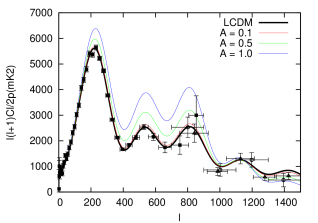
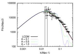
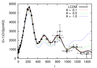
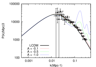
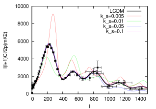
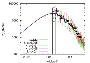
First let us consider the case of the slope change. It is rather straightforward to predict the CMB and matter power spectra. As shown in the left panel of Figure 1, there is a power modulation on the small scale for $\mathcal{P}(k)$, depending on the sign of the slope change. Consequently, we expect that the CMB and matter power spectra would show the corresponding change in power. In the upper panel of Figure 4, we set the position of the slope change to be $0.05\mathrm{Mpc}^{-1}$ and give a few positive changes. On the left panel where the CMB spectrum is shown, we can see clearly that there is an enhancement up to $l\sim 800$ when the slope changes positively. The corresponding matter power spectrum is on the right side. Compared with the large scale, the power on small $k$ is decreased drastically as the slope change becomes bigger. In opposite, there is an enhancement on small scales if the change is negative, as shown in the lower row of Figure 4. Taking matter power spectra into account, such an enhancement is more prominent. For both cases, the diminishing oscillatory behaviour is not noticeable in the CMB spectra, since the background CMB spectrum is also oscillating. Rather, it is clearly shown in the matter power spectra in the small $k$ region.

Figure 5: (Left column) plots of the CMB and (right column) matter power spectra with (upper row) positive and (lower row) negative slope change, depending on the position of the slope change $k_{0}$. The size of the slope change is set to $|\Delta A/A|=0.5$.

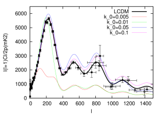
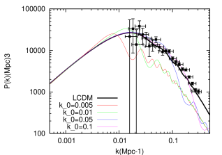
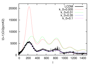
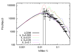
We can also ask the dependence on the position of the slope change. If the slope changes early enough, it would affect most of the observationally relevant scales, and the CMB and matter power spectra should be very different from those we actually observed. The effects of various positions of the slope change are given in Figure 5. As anticipated, when the slope change happens before the largest observable scale, power spectra are largely enhanced or suppressed on most of the scale.

Figure 6: (Left column) plots of the CMB and (right column) matter power spectra corresponding to the sharp downward step in $V(\phi)$. In the upper row $k_{s}$ is fixed at $0.05\mathrm{Mpc}^{-1}$, and in the lower row the magnitude of the step is fixed to be $B=0.5$ but the position $k_{s}$ is varying.

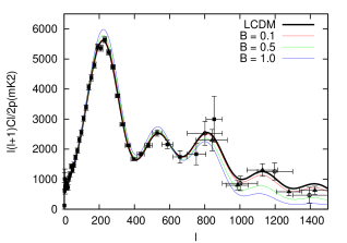
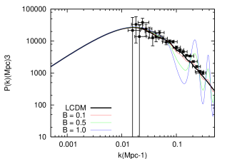
Now we transfer our attention to the case of the step. Before we present the results, let us pause for a moment and anticipate the associated spectra by considering the form of $\mathcal{P}(k)$ in Figure 2. It is clear that around the scale $k_{s}$, which corresponds to the position of the step, first we see that after a slight enhancement, there is a large suppression in the power, and then oscillation. So, the CMB and matter power spectra should first experience a suppression, and then oscillate. One thing here we should bear in mind is the value of $k_{s}$. If $k_{s}$ is large, that is, if the step appears quite lately, many of the relevant scales would have already crossed the horizon and there would be no prominent difference. Conversely, when $k_{s}$ is small, i.e., most of the observationally important scales have gone through the step, the oscillatory behaviour of $\mathcal{P}(k)$ would have been obviously imprinted on the spectra we see today when the step is sharp enough. In the upper row of Figure 6 $k_{s}$ is fixed to be $0.05\mathrm{Mpc}^{-1}$ and the size of the step varies. In the CMB spectrum on the left side it is shown that on small $l$ the power is slightly greater, but on large $l$ it becomes smaller. The oscillatory feature is manifest in the matter power spectrum in the right panel of Figure 6. The dependence of the CMB and matter power spectra on $k_{s}$ is depicted in the lower row of Figure 6. As expected, when $k_{s}$ is large, it is almost the same with the background $\Lambda$CDM cosmology. But if $k_{s}$ is small enough to affect the whole observable scales, the departure from the usual $\Lambda$CDM is very large. Note that for the case of smoothed step, only the first few oscillations in the matter power spectrum survive and the rest quickly diminish, as shown in Figure 2.

4.2 Degeneracy

As we have seen in the previous section, the distortions of the observable CMB and matter power spectra are dependant on both the magnitude and the position of the feature. Of these, the magnitude of the feature is tightly constrained to be very small by cosmological observations on the CMB and galaxy distribution. If the size were to be large enough to have been imprinted on the observable spectra, we would already have noticed a large departure from scale invariance on various scales. For example, the fractional change in the inflaton potential amplitude of about $0.1\%$ for the smoothed hyperbolic tangent step, i.e., $a\sim 0.001$, is known to cause sufficient sharp features in the CMB spectrum [11, 23]. Yet, it seems more difficult to put strong constraints on the position of the feature.

Figure 7: The differences in the CMB power spectra between the models with a step and the background $\Lambda$CDM, $C_{l}(\mbox{step models in the lower row of Figure~{}\ref{step}})-C_{l}(\Lambda\mathrm{CDM})$.

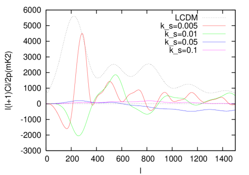
In the light of this, it seems not impossible to mimic some cosmological model by introducing a feature to another one with different parameters. That is, provided that the size is small enough, we may have strong degeneracies between cosmological models depending on appropriate position of the feature. In particular, by the CMB spectrum alone, we are possibly led to determine the cosmological parameters incorrectly, since the oscillatory period in the CMB spectrum might overlap with that of the feature. In Figure 7, we show the difference between the CMB spectrum of the background $\Lambda$CDM and those of the models with steps at various positions. We see that a step at some position slightly smaller than $k_{s}\sim 0.01\mathrm{Mpc}^{-1}$ gives a similar oscillatory cycle. Also, $k_{s}\lesssim 0.05\mathrm{Mpc}^{-1}$ seems to enhance the first peak slightly, but lower the subsequent ones.

For example, in Figure 8, we show the CMB and matter power spectra of two different models. One model, with a scale invariant primordial spectrum, is provided by the background $\Lambda$CDM, while the other has a sharp downward step at $k_{s}=0.01\mathrm{Mpc}^{-1}$ with $B=0.1$, where the cosmological parameters are set to $\Omega_{\mathrm{B}}=0.040,\Omega_{\mathrm{DM}}=0.200$ and $\Omega_{\Lambda}=0.760$. In this case, the position and the height of the first peak are very similar for the two CMB spectra, making them not easily distinguishable. However, in the matter power spectra we can note an oscillation in the power in the small $k$ region, leaving some scope for discrimination.

Figure 8: Power spectra of the background $\Lambda$CDM and a step model where $\Omega_{\mathrm{B}}=0.040,\Omega_{\mathrm{DM}}=0.200$ and $\Omega_{\Lambda}=0.760$. The first peaks of the two CMB spectra are nearly the same.

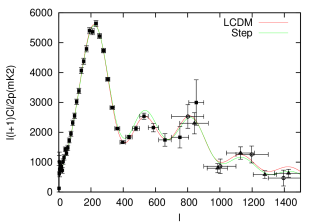
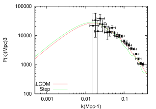
Another example is given in Figure 9, where again the background $\Lambda$CDM is shown for comparison. Here we take $B=0.1$ and $k_{s}=0.04\mathrm{Mpc}^{-1}$, and the parameters $\Omega_{\mathrm{B}}=0.060,\Omega_{\mathrm{DM}}=0.390,\Omega_{\Lambda}=0.550$ and $h=0.62$. While the cosmological parameters are quite different, the CMB peaks and troughs roughly overlap in this example. It seems that even if we could measure the CMB spectrum with very high accuracy by some experiments, e.g., using the planned Planck surveyor, we should be very cautious to abandon any featured primordial spectrum and choose the precisely flat, scale invariant one confidently.

Figure 9: Power spectra of the background $\Lambda$CDM and a step model where $\Omega_{\mathrm{B}}=0.060,\Omega_{\mathrm{DM}}=0.390,\Omega_{\Lambda}=0.550$ and $h=0.62$. Both the two CMB power spectra seem well within the error bars in the CMB spectrum observation. Can we distinguish these two models with the CMB observation alone?

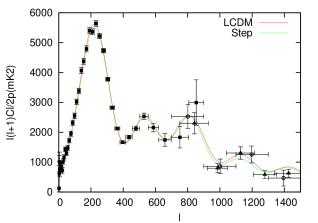
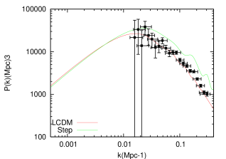
Therefore it is very likely that with the CMB observation alone, where the usually assumed scale invariant $\mathcal{P}(k)$ of the standard $\Lambda$CDM and the scale dependent $\mathcal{P}(k)$ from the inflaton potential with a step generate very similar CMB power spectra despite the different cosmological parameters, we are led to confusion for the parameter estimation. Such degeneracies would only be broken by combining some other observations, e.g., a matter power spectrum, as shown in Figure 9. But when the step is not infinitely sharp but mild, which is supposed to be a more realistic case, the oscillation quickly dies away, except a first couple of peaks, back to the background value. This should make discrimination difficult in the matter power spectrum observations as well.

5 Conclusions

In many extensions of the standard model of particle physics, e.g., supersymmetry and string theory, the existence of many scalar fields is predicted. During inflation which such theories would have described correctly, more than one scalar field may have been relevant. In this regards, it is meaningful to investigate the effect of inflaton potential with some feature which is produced generically by spontaneous symmetry breaking of another scalar field coupled to inflaton. The corresponding power spectrum of curvature perturbations $\mathcal{P}(k)$ generally deviates from the usually adopted flat, scale invariant one.

In this paper, we have considered the primordial power spectrum of curvature perturbations which arises from some potential with a feature due to spontaneous symmetry breaking of another scalar field coupled to inflaton field. On the basis of the general slow-roll approximation, we can proceed in a systematic and organised manner with the calculation of the curvature power spectrum $\mathcal{P}(k)$, and indeed in Section 3 we have obtained fully analytic results of $\mathcal{P}(k)$ in various situations. Generally, such a feature leads to the breaking of scale invariance of $\mathcal{P}(k)$, which is given as an oscillatory behaviour in $\mathcal{P}(k)$ on scales smaller than those associated with the position of the feature, accompanied with an overall modulation of the power when $V(\phi)$ becomes flatter or steeper. Given such a power spectrum, we also have obtained the associated CMB and matter power spectra which we can actually observe. When the magnitude of the feature is large and its position corresponds to large scale, both the oscillation and power modulation imprinted in $\mathcal{P}(k)$ are noticeable in the CMB and matter power spectra.

One expectation we could draw from the above results is that it might be possible to mimic some cosmological model with a scale invariant primordial power spectrum $\mathcal{P}(k)$ with a scale dependent $\mathcal{P}(k)$ resulting from some featured inflaton potential in spite of different cosmological parameters such as $\Omega_{\mathrm{B}},\Omega_{\mathrm{DM}},\Omega_{\Lambda}$ and $h$. Such a degeneracy is especially strong for the CMB power spectrum, since the oscillatory period of $\mathcal{P}(k)$ may overlap with that of the CMB peaks, depending on the magnitude and the position of the feature in $V(\phi)$. In this regard, we believe that close investigations of independent observations, e.g., the matter power spectrum or supernovae, would remove our potential confusion as regards the cosmological parameter estimates. It might also provide interesting theoretical possibilities for the particle physics responsible for the generation of the feature in $V(\phi)$. Tight observational bounds on the magnitude and the position of the feature would constrain the particle physics model behind the inflaton potential as well, shedding some light on our understanding of the universe.

Acknowledgements

I thank Kiwoon Choi, Jai-chan Hwang, Donghui Jeong, Kang Young Lee, Carlos Muñoz, Subir Sarkar, Misao Sasaki and Ewan Stewart for many helpful discussions and important suggestions. Especially I am indebted to Richard Easther for invaluable comments on the CMB spectrum. This work was supported in part by ARCSEC funded by the KOSEF and the Korean Ministry of Science and the KRF grant PBRG 2002-070-C00022.

References

- [1] A. A. Starobinsky, Phys. Lett. B 91, 99 (1980) ; A. H. Guth, Phys. Rev. D 23, 347 (1981) ; A. D. Linde, Phys. Lett. B 108, 389 (1982) ; A. Albrecht and P. J. Steinhardt, Phys. Rev. Lett. 48, 1220 (1982)
- [2] V. F. Mukhanov and G. V. Chibisov, JETP Lett. 33, 532 (1981) ; S. W. Hawking, Phys. Lett. B 115, 295(1982) ; A. H. Guth and S.-Y. Pi, Phys. Rev. Lett. 49, 1110 (1982) ; A. A. Starobinsky, Phys. Lett. B 117, 175 (1982) ; J. M. Bardeen, P. J. Steinhardt and M. S. Turner Phys. Rev. D 28, 679 (1983)
- [3] V. F. Mukhanov, H. A. Feldman and R. H. Brandenberger, Phys. Rept. 215, 203 (1992)
- [4] D. N. Spergel et al., Astrophys. J. Suppl. 148, 175 (2003) astro-ph/0302209
- [5] S. Dodelson and E. Stewart, Phys. Rev. D 65, 101301 (2002) astro-ph/0109354 ; E. D. Stewart, Phys. Rev. D 65, 103508 (2002) astro-ph/0110322 ; J.-O. Gong, Class. Quant. Grav. 21, 5555 (2004) gr-qc/0408039
- [6] J. Choe, J.-O. Gong and E. D. Stewart, JCAP 07, 012 (2004) hep-ph/0405155
- [7] D. S. Salopek, J. R. Bond and J. M. Bardeen, Phys. Rev. D 40, 1753 (1989)
- [8] A. A. Starobinsky, JETP Lett. 55, 489 (1992)
- [9] M. Kamionkowski and A. R. Liddle, Phys. Rev. Lett. 84, 4525 (2000) astro-ph/9911103
- [10] S. M. Leach and A. R. Liddle, Phys. Rev. D 63, 043508 (2001) astro-ph/0010082 ; S. M. Leach, M. Sasaki, D. Wands and A. R. Liddle, Phys. Rev. D 64, 023512 (2001) astro-ph/0101406
- [11] J. A. Adams, B. Cresswell and R. Easther, Phys. Rev. D 64, 123514 (2001) astro-ph/0102236
- [12] P. Hunt and S. Sarkar, Phys. Rev. D 70, 103518 (2004) astro-ph/0408138
- [13] C. R. Contaldi, M. Peloso, L. Kofman and A. Linde, JCAP 07, 002 (2003) astro-ph/0303636
- [14] J. A. Adams, G. G. Ross and S. Sarkar, Nucl. Phys. B 503, 405 (1997) hep-ph/9704286
- [15] A. D. Linde, Phys. Rev. D 49, 748 (1994) astro-ph/9307002
- [16] E. D. Stewart and J.-O. Gong, Phys. Lett. B 510, 1 (2001) astro-ph/0101225 ; J.-O. Gong and E. D. Stewart, Phys. Lett. B 538, 213 (2002) astro-ph/0202098
- [17] M. Joy, E. D. Stewart, J.-O. Gong and H.-C. Lee, JCAP 04, 012 (2005) astro-ph/0501659
- [18] U. Seljak and M. Zaldarriaga, Astrophys. J. 469, 437 (1996) astro-ph/9603033
- [19] J. Lesgourgues, D. Polarski and A. A. Starobinsky, Mon. Not. Roy. Astron. Soc. 297, 769 (1998) astro-ph/9711139
- [20] T. J. Pearson et al., Astrophys. J. 591, 556 (2003) astro-ph/0205388
- [21] C.-L. Kuo et al., Astrophys. J. 600, 32 (2004) astro-ph/0212289
- [22] M. Tegmark et al., Astrophys. J. 606, 702 (2004) astro-ph/0310725
- [23] H. V. Peiris et al., Astrophys. J. Suppl. 148, 213 (2003) astro-ph/0302225
- [24] A. Blanchard, M. Douspis, M. Rowan-Robinson and S. Sarkar, Astron. Astrophys. 412, 35 (2003) astro-ph/0304237