A Simple and Accurate Model for Intra-Cluster Gas

Abstract

Starting with the well-known NFW dark matter halo distribution, we construct a simple polytropic model for the intracluster medium which is in good agreement with high resolution numerical hydrodynamical simulations, apply this model to a very large scale concordance dark matter simulation, and compare the resulting global properties with recent observations of X-ray clusters, including the mass-temperature and luminosity-temperature relations. We make allowances for a non-negligible surface pressure, removal of low entropy (short cooling time) gas, energy injection due to feedback, and for a relativistic (non-thermal) pressure component. A polytropic index $n=5$ ($\Gamma=1.2$) provides a good approximation to the internal gas structure of massive clusters (except in the very central regions where cooling becomes important), and allows one to recover the observed $M_{500}-T$, $L_{x}-T$ and $T/n_{e}^{2/3}\propto T^{0.65}$ relations. Using these concepts and generalizing this method so that it can be applied to fully three-dimensional N-body simulations, one can predict the global X-ray and SZE trends for any specified cosmological model. We find a good fit to observations when assuming that twelve percent of the initial baryonic mass condenses into stars, the fraction of rest mass of this condensed component transferred back to the remaining gas (feedback) is $3.9\times 10^{-5}$, and the fraction of total pressure from a nonthermal component is near ten percent.

1 Introduction

Gas in clusters of galaxies can be observed to large cosmological distances by a variety of techniques, from X-rays (Bremsstrahlung) to radio (S-Z effect). But to utilize these observations it is necessary to have a model for the state of the gas in clusters that is (a) motivated by sound physical reasons, (b) able to fit the observational data and (c) is simple enough (i.e., not a numerical simulation!) to be applied broadly. In this paper we attempt to present such a model for the gaseous component in clusters of galaxies in order to provide predictions for global properties such as temperature and X-ray luminosity.

For the dark matter (DM), the widely utilized Navarro, Frenk & White (1997), or NFW, model satisfies all of the above criteria. Although we now know that it is not universal in two senses— large variance in the central concentrations (Avila-Reese et al., 1999; Jing, 2000; Bullock et al., 2001; Klypin et al., 2001; Fukushige, Kawai & Makino, 2004; Tasitsiomi, et al., 2004) and trends in properties with time and halo mass (Wechsler et al., 2002; Ricotti, 2003; Zhao et al., 2003; Weller, Ostriker & Bode, 2005; Salvador-Sole, Manrique & Solanes, 2005)— it remains an extremely useful first basis for analyzing and summarizing the properties of dark matter distributions. We know, however that the gas in clusters does not follow the dark matter profile. The well established central density profiles for dark matter halos are roughly power laws: density $\rho$ depends on radius $r$ as $\rho\propto r^{-\alpha}$, with $\alpha$ typically 1.0 (the NFW value) but ranging from 0.5 to 1.5, depending on circumstances. But the gas profiles show a definite core ($\alpha\rightarrow 0$; for a recent review see Voit, 2004) and, as we shall see, one would overestimate the X-ray luminosity by a large factor if one were to use the NFW or a steeper profile.

The construction of a satisfactory model will be guided by a few observed properties. First, the gas is essentially a trace component (approximately 1/7 of total mass) and resides, in close to hydrostatic equilibrium, in a potential which is well represented by NFW (or its variants– cf. Zhao, 1996). Furthermore, we know that there are efficient means of redistributing energy/entropy within the cluster gas via, for example, turbulence (Kim & Narayan, 2003b) induced by merger shocks (Bryan & Norman, 1998) and galaxy wakes (Stevens, Acreman & Ponman, 1999; Sakelliou, 2000). Additionally, other processes such as conduction (Kim & Narayan, 2003a; Dolag et al., 2004), cosmic ray transport, and magneto-sonic wave transport (Cen, 2005) may also be operating. Also, appropriate boundary conditions are required, since in both simple analytic models (eg. Bertschinger, 1985) and detailed numerical simulations (eg. Bryan & Norman, 1998; Frenk et al., 1999) the hydrostatic portion of the cluster gas is terminated at an outer shock where the pressure is balanced by the momentum flux of the infalling gas.

A number of steps have already been made toward constructing such a model. Makino, Sasaki & Suto (1998) derived an analytic expression for a gas distribution in hydrostatic equilibrium with an NFW potential, assuming isothermality. A more general expression for a polytropic equation of state was derived by Suto et al. (1998); a similar functional form has been compared in detail with hydrodynamic simulations by Ascasibar et al. (2003).

In the simplest of such models the source of the gas heating is gravitational, i.e. the gas energy comes from the same collapse and virialization processes which determine the dark matter profile; thus the energy per unit mass in the gas should be approximately the same as in the dark matter. This leads to an expected self-similar scalings of mass $M$ and luminosity $L$ with temperature $T$ of $M\propto T^{3/2}$ and $L\propto T^{2}$ (Kaiser, 1986). However, this expectation is in contradiction with the observed relation, which is steeper (Edge & Stewart, 1991; Markevitch, 1998). Kaiser (1991) proposed that non-gravitational energy injection could lead to the observed relations. This possibility has been explored in the type of analytic model described here using an NFW profile for the dark matter (Suto et al., 1998; Wu, Fabian & Nulsen, 2000; Shimizu et al., 2004; Lapi, Cavaliere & Menci, 2005; Afshordi, Lin & Sanderson, 2005; Solanes et al., 2005), and with other profiles (Balogh, Babul & Patton, 1999; Babul et al., 2002). The breaking of self-similarity can also be cast as the modification of the initial gas entropy by thermal and nonthermal processes, as explored in NFW-like potentials by Tozzi & Norman (2001), Komatsu & Seljak (2001), Voit et al. (2002), and Dos Santos & Doré (2002); on the other hand Roychowdhury & Nath (2003) argue that the entropy imparted to the gas from gravitational processes alone is larger than previously thought. Another impact on the gas energy comes from the fact that approximately one tenth of the baryons in a typical cluster are now in stellar form. So one must allow for both removal of the mass of this gas and of the associated energy (or entropy) of this gas (Voit & Bryan, 2001; Tozzi & Norman, 2001; Voit et al., 2002; Scannapieco & Oh, 2004; Bryan & Voit, 2005). Since the removed gas had short cooling times, low entropy, and low total energy, the mean energy per unit mass of the remaining gas is higher than before star and galaxy formation.

An issue not dealt with in these studies is non-thermal sources of pressure. Turbulence may provide in excess of 10% of the total pressure in Coma (Schuecker et al., 2004); similar amounts of turbulent support have been seen in simulations (Norman & Bryan, 1999; Faltenbacher et al., 2004). Clusters should also contain a population of relativistic particles arising from shocks, as recently reviewed by Miniati (2004), Sarazin (2004), and Bykov (2005). Magnetic fields may also be dynamically important (Carilli & Taylor, 2002; Ensslin, Vogt & Pfrommer, 2005; Bykov, 2005).

The basic goal of this paper is to start with a population of dark matter halos from an N-body simulation, for which the DM density profiles can easily be measured, and deduce the global properties of the hot baryonic component in a physically well-motivated manner. The ideal method should be as simple as possible while including all the relevant components: hydrostatic equilibrium inside a dark matter halo potential; gas energy per unit mass similar to that of the dark matter, but modified by removal of low entropy gas and by feedback; appropriate outer boundary conditions; and pressure support from a non-thermal component. Some other processes necessary for detailed models will not be included because they are not in general required for obtaining global properties; though the results obtained here may need to be modified for those clusters having distinctly cooler cores (Allen & Fabian, 1998). Finally, we will drop the limitation of a spherical NFW model and generalize to any case for which the dark matter potential is known. While several of the papers quoted above have allowed for some of these effects, none has included all in a fashion that can be adapted to an arbitrary gravitational potential.

The next section reviews properties of the NFW model; §3 derives the properties of an initially parallel gaseous component and §4 derives these properties after the gas rearranges itself; §5 presents the resulting profiles and compares global properties with observed clusters. All of these sections assume spherical symmetry. In §6 we generalize the polytropic model in order to remove geometrical constraints, concluding our discussion in §7.

2 The NFW Profile

Navarro, Frenk & White (1997) have proposed a universal profile for dark matter halos, which we will first review here to establish nomenclature. Formally, the NFW profile extends to infinity and has logarithmically diverging mass; we will instead truncate the profile at the virial radius. In this section we first establish the properties of a distribution of matter with a truncated NFW profile. Assume that the density $\rho$ depends on radius $r$ as

$$\rho(r)=\left\{\begin{array}[]{ll}\frac{\rho_{1}r_{1}^{3}}{r(r+r_{1})^{2}}&r\leq r_{v}\hskip 28.45274pt,\\ 0&r>r_{v}\hskip 28.45274pt.\end{array}\right.$$ (1)

The virial radius $r_{v}$ is the radius within which the mean density is 200 times the critical density $\rho_{c}$. The parameters $C\equiv r_{v}/r_{1}$ and $\rho_{1}$ define the model. It follows that the mass $M$ is distributed inside $r_{v}$ as:

$$M(r) = 4\pi\ \rho_{1}r_{1}^{3}\ g(x)\hskip 28.45274pt,$$ (2a)

$$g(x) \equiv \ln(1+x)-\frac{x}{(1+x)}\hskip 28.45274pt,$$ (2b)

where $x\equiv r/r_{1}$. Thus $M_{tot}\equiv M(r_{v})=4\pi\ \rho_{1}r_{1}^{3}\ g(C)$ is the total mass. The rotation curve, $V_{c}^{2}(r)=GM(r)/r=4\pi G\rho_{1}r_{1}^{2}g(x)/x$ provides a useful label for the mass distribution; it has a maximum at $x_{c,max}\approx 2.163$, so the maximum circular velocity is

$$V_{c,max}^{2} = 4\pi G\rho_{1}r_{1}^{2}G_{max}\hskip 28.45274pt,$$ (3a)

$$G_{max} \equiv g(x_{c,max})/x_{c,max}\approx 0.2162\hskip 28.45274pt.$$ (3b)

Note that a given $M_{tot}$ and $V_{c,max}$ can be used to completely define the matter distribution (as an alternative to $C$ and $\rho_{1}$).

The gravitational potential from this mass distribution is

$$\Phi(x)=-\frac{V_{c,max}^{2}}{G_{max}}f(x)\hskip 28.45274pt,$$ (4)

where

$$f(x)=\left\{\begin{array}[]{ll}\frac{\ln(1+x)}{x}-\frac{1}{1+C}&x\leq C\\ \left[\frac{\ln(1+C)}{C}-\frac{1}{1+C}\right]\frac{C}{x}&x>C\\ \end{array}\hskip 28.45274pt\right.$$ (5)

The total gravitational energy is then given by

$$W_{0}=\frac{1}{2}\int_{0}^{M_{tot}}{\Phi(r)dM}=-G_{max}^{-1}V_{c,max}^{2}M_{tot}H(C)\hskip 28.45274pt,$$ (6a)

where

$$H(C)\equiv\left[-\frac{\ln(1+C)}{(1+C)}+\frac{C(1+C/2)}{(1+C)^{2}}\right]\frac{1}{g(C)}\hskip 28.45274pt.$$ (6b)

Assuming velocities are isotropic for the bulk of the matter distribution, the velocity dispersion of the dark matter in 1-D, $\sigma^{2}(r)$, obeys the equation $\frac{d}{dr}(\rho\sigma^{2})=-\rho\frac{d}{dr}\Phi$, which has the solution

$$\sigma^{2}=\frac{V_{c,max}^{2}}{G_{max}}S_{C}(x)x(1+x)^{2}\hskip 28.45274pt,$$ (7a)

where

$$S_{C}(x)=S_{C}(C)-\int_{x}^{C}{\frac{x^{\prime}-(1+x^{\prime})\ln(1+x^{\prime})}{x^{\prime 3}(1+x^{\prime})^{3}}}dx^{\prime}\hskip 28.45274pt,$$ (7b)

with $S_{C}(C)$ a positive constant, the value of which will be determined below. The corresponding pressure is simply $P=\rho\sigma^{2}=4\pi G\rho_{1}^{2}r_{1}^{2}S_{C}(x)$, so the average pressure is

$$\overline{P}=\frac{1}{\frac{4}{3}\pi r_{v}^{3}}\int_{0}^{r_{v}}{Pd{\bf r}}={12\pi G\rho_{1}^{2}r_{1}^{2}C^{-3}}\int_{0}^{C}{S_{C}(x)x^{2}dx}\hskip 28.45274pt,$$ (8a)

and the surface pressure is

$$P_{s}=4\pi G\rho_{1}^{2}r_{1}^{2}S_{C}(C)\hskip 28.45274pt.$$ (8b)

A boundary surface pressure is required because of the jump in density and pressure at $r=r_{v}$, and would be provided in any realistic physical model by the momentum flux from infalling matter at the boundary. One way to quantify the pressure term represented by $S_{C}(C)$ is to estimate the momentum per unit area transported in by infalling matter. If the rate of mass accretion is $\dot{M}_{tot}$ and the accreted mass (starting at rest from the turnaround radius) is moving at freefall velocity $v^{2}_{ff}=V^{2}_{c}(r_{v})$, then $P_{s}=\dot{M}_{tot}v_{ff}/(4\pi r_{v}^{2})$. In the self-similar solution of Bertschinger (1985) $M_{tot}\propto t^{2/3}$. This should be approximately correct, so we will take $\dot{M}_{tot}=2qM_{tot}/(3t)$, with deviations allowed for with use of the correction factor $q$. Clusters of galaxies are by definition in overdense regions, so the surroundings will always appear to be close to the critical density $\rho_{c}$, hence an appropriate time is $t=(6\pi G\rho_{c})^{-1/2}$; thus we will adopt

$$P_{s}=\frac{\sqrt{2}}{3}qV^{2}_{c}(r_{v})\rho_{s}\left(\frac{\rho_{c}}{\rho_{s}}\frac{\bar{\rho}}{\rho_{s}}\right)^{1/2}\hskip 28.45274pt,$$ (9)

where $\rho_{s}$ is the density at $r_{v}$, and $\bar{\rho}$ is the mean density inside $r_{v}$. Combining this with Eqn. (8b), it follows that

$$S_{C}(C)=\left(\frac{2}{3}q^{2}\frac{g^{3}(C)}{C^{5}}\frac{\rho_{c}}{\rho_{1}}\right)^{1/2}=\sqrt{2}q\frac{g^{2}(C)}{C^{4}}\left(\frac{\bar{\rho}}{\rho_{c}}\right)^{-1/2}=q\frac{g^{2}(C)}{10C^{4}}\hskip 28.45274pt.$$ (10)

Alternatively, one may take the expression for the radial velocity dispersion in an NFW halo derived by Lokas & Mamon (2001) and evaluate it at the virial radius $x=C$. Lokas & Mamon (2001) solved the Jeans equation for an NFW density profile assuming a constant velocity anisotropy; for the simplest case of isotropic orbits, their Eqn. (14) yields

$$\begin{array}[]{c}S_{C}(C)=\frac{\pi^{2}}{2}-\frac{{\rm ln}C}{2}-\frac{1}{2C}-\frac{1}{2(1+C)^{2}}-\frac{3}{1+C}+\left(\frac{1}{2}+\frac{1}{2C^{2}}-\frac{2}{C}-\frac{1}{1+C}\right){\rm ln}(1+C)+\\ \frac{3}{2}{\rm ln}^{2}(1+C)+3{\rm Li}_{2}(-C)\end{array}$$ (11)

with the dilogarithm Li${}_{2}(x)=\int_{x}^{0}{\rm ln}(1-y)d{\rm ln}y$. For the low concentration halos considered here, this gives pressures similar to Eqn. (10) with $q\approx 4$. We will use Eqn. (11) in the following, but have found simply using $q=4$ gives very similar results. An intriguing feature of the NFW model is that the coarse-grained phase space density $\rho(x)/\sigma^{3}(x)$ is a power law in radius, following $x^{-15/8}$ (Taylor & Navarro, 2001; Williams et al., 2004). Using Eqn. (11) to set the surface pressure, the phase space density found by combining Eqns. (1) and (7a) does display in this power law behavior, with the appropriate slope. If we instead use (for example) $q=1$, then the same power law still holds inside $0.5r_{v}$; only nearer the surface is there a significant deviation. This insensitivity to the exact choice of surface pressure helps explain why the approximation $q\approx 4$ works well.

3 Initial Gas Energy and Pressure

The goal of this paper is to populate with gas, in a physically plausible fashion, the potential well created by a dark matter halo with known mass, radius, concentration, and maximum circular velocity. Let the ratio of initial gas mass to total mass equal the cosmic average, i.e. the total gas mass $M_{g,i}=\Omega_{b}M_{tot}/\Omega_{m}$. We begin by assuming that initially the two components have a parallel distribution— which is what would be expected in the absence of energy transport mechanisms. Thus the gas pressure is by hypothesis $P_{g}=(M_{g,i}/M_{tot})P$.

Now we apply the Virial Theorem to the whole, with allowance for the non-negligible surface pressure: $W_{0}+2T_{0}-4\pi r_{v}^{3}P_{s}=0$. Since the kinetic energy $T_{0}$ is related to the mean pressure (in the absence of significant bulk motions) by $2T_{0}=4\pi r_{v}^{3}\overline{P}$, we have, using Eqn. (8a),

$$W_{0}=-4\pi r_{v}^{3}\left(\overline{P}-P_{s}\right)=-3\langle\sigma^{2}\rangle M_{tot}(1-\delta_{s})\hskip 28.45274pt,$$ (12)

where $\delta_{s}\equiv P_{s}/\bar{P}$ is the surface pressure in terms of the mean. When combined with Eqn. (6a), this becomes

$$3\langle\sigma^{2}\rangle(1-\delta_{s})=G_{max}^{-1}V_{c,max}^{2}H(C)\hskip 28.45274pt.$$ (13)

Note this is taken from the definition of $\langle\sigma^{2}\rangle\equiv\int{\sigma^{2}dM}/M_{tot}=(\frac{4}{3}\pi r_{v}^{3}\overline{P})/M_{tot}$. Rewriting Eqn. (13) using Eqns. (6a) and (7a) gives the dimensionless form of the Virial Theorem:

$$3(1-\delta_{s})\int_{0}^{C}{S_{C}(x)x^{2}dx}=H(C)g(C)\hskip 28.45274pt.$$ (14)

It follows that

$$\delta_{s}=\frac{S_{C}(C)}{S_{C}(C)+C^{-3}H(C)g(C)}\hskip 28.45274pt.$$ (15)

Given $S_{C}(C)$, $\delta_{s}$ is known, and Eqn. (13) can be rewritten as $\langle\sigma^{2}\rangle=K(C)V_{c,max}^{2}$, where

$$K(C)=\frac{1}{3}H(C)\frac{G_{max}^{-1}}{(1-\delta_{s})}\hskip 28.45274pt,$$ (16)

and the potential energy from Eqn. (6a) is now

$$W_{0}=-3K(C)(1-\delta_{s})M_{tot}V_{c,max}^{2}\hskip 28.45274pt.$$ (17)

Thus the kinetic and potential energies can be specified, once the NFW parameters for a dark matter halo have been specified.

Earlier we assumed a monatomic gas component, initially distributed in the same manner as the dark matter. What is the total energy of the gas? Treating it as a tracer of negligible mass, that is, assuming the gravitational potential is totally determined by the dark matter, $E_{g}=\text@frac{1}{2}M_{g,i}\langle 3\sigma^{2}\rangle+2\left({M_{g,i}}/{M_{tot}}\right)W_{0}$. Combining this with Eqn. (17) gives

$$E_{g}=-\frac{3}{2}M_{g,i}V_{c,max}^{2}K(C)(3-4\delta_{s})\hskip 28.45274pt.$$ (18)

Also, the gas surface pressure from Eqns. (8b) and (3a) is

$$P_{s,gas}=\frac{M_{g,i}V_{c,max}^{2}}{4\pi r_{1}^{3}}\frac{S_{C}(C)}{G_{max}g(C)}\hskip 28.45274pt.$$ (19)

Thus both the gas energy and surface pressure are now known in terms of the dark matter halo parameters.

3.1 Allowance for Stellar Mass Dropout

Star formation will change the amount of energy in the remaining gas, because that portion of the the gas which collapses and is removed will have a lower entropy and a shorter cooling time than is typical. In our idealized halo, this is the gas which would end up in the central region, so we will estimate the change in energy by removing a fraction of the core; this removed fraction (corresponding to the mass in stars) has the shortest cooling time and lowest entropy. Fukugita, Hogan & Peebles (1998) estimated that for clusters the stellar mass inside the virial radius is roughly 0.19$h^{0.5}$ times the gas mass, and Sanderson & Ponman (2003) find a median stellar to gas ratio of 0.21; but lower values have been found by Balogh et al. (2001) and Lin, Mohr & Stanford (2003). We will adopt a stellar to gas mass ratio of 0.12 independent of cluster mass, in reasonable agreement with the results of the latter two papers, assuming a LCDM model with $h$=0.7. For simplicity we will assume enough gas is turned into stars for this ratio to hold generally. In other words, the ratio of the mass in stars to the final gas mass is $f_{s}=0.12$, with $M_{g}=M_{g,i}/(1+f_{s})$ remaining in the gaseous state. This will be done by removing all gas inside a radius $x_{s}$, found by solving $g(x_{s})=g(C)f_{s}/(1+f_{s})$. The initial energy in this remaining gas is found by integrating the previous expressions for the energy over only the mass $M_{g}$ outside of $x_{s}$:

$$E_{g}=-\frac{3}{2}(1+f_{s})M_{g}V_{c,max}^{2}\left[K(C)(3-4\delta_{s})+K_{s}(x_{s})/G_{max}\right]$$ (20)

with

$$K_{s}(x_{s})=\frac{1}{g(C)}\left[\int_{0}^{x_{s}}S_{C}(x)x^{2}dx-\frac{2}{3}\int_{0}^{x_{s}}\frac{f(x)xdx}{(1+x)^{2}}\right]$$ (21)

which, while unfortunately not as simple as before, can still be determined once the dark matter halo parameters are given. By removing this gas we are both lowering the gas mass and, more critically, increasing the energy per unit mass of the remaining gas (Voit & Bryan, 2001).

3.2 Other Changes to the Gas Energy

The gas energy will change due to the the work done by any increase or decrease of the gas volume. To calculate this latter term, we will assume that the surface pressure does not change with radius, i.e. it is always given by Eqn. (19). Let $C_{f}$ be the final outer radius of the gas distribution in units of $r_{1}$; then

$$\Delta E_{P}=-\frac{4\pi}{3}r^{3}_{1}\left(C^{3}_{f}-C^{3}\right)P_{s,gas}(C)=-\frac{1}{3}(1+f_{s})M_{g}V_{c,max}^{2}\left(C^{3}_{f}-C^{3}\right)\frac{S_{C}(C)}{G_{max}g(C)}\hskip 28.45274pt.$$ (22)

In addition, we can expect there to be energy input to the gas from feedback processes. These are primarily of two kinds: wind and supernova shock energy deposited in the hot gas, and heating due to output from accreting massive black holes in the centers of the massive galaxies (Scannapieco & Oh, 2004). Dynamical friction on galaxies moving through the gas at somewhat trans-sonic speeds may also be a source of energy input (Ostriker, 1999; El-Zant, Kim & Kamionkowski, 2004; Faltenbacher et al., 2004). To a good first approximation all of these effects are proportional to the gas mass (there is no evidence that the efficiency with which gas is transferred to stars varies strongly and systematically with $V^{2}_{c,max}$ for moderately rich clusters). Let $\epsilon$ be a measure of the efficiency with which gas is heated by the condensed component; the energy input can then be written as

$$\Delta E_{f}=\epsilon f_{s}M_{g}c^{2}\hskip 28.45274pt.$$ (23)

The value of $\epsilon$ from energy output of supernovae can be estimated as the product of the fraction of mass turned into stars ($f_{s}$=0.12), the number of supernovae per solar mass expected from a Salpeter initial mass function ($0.007M_{\odot}^{-1}$), and the energy input per supernova ($10^{51}$ erg); this gives $\epsilon=2.8\times 10^{-6}$ or $\epsilon f_{s}=3\times 10^{-7}$. While assuming perfect efficiency in transferring this energy into the gas is unrealistic, we find that by itself this amount of energy has little impact on the gas profile, consistent with previous results (Balogh, Babul & Patton, 1999; Valageas & Silk, 1999; Bower et al., 2001; Shimizu et al., 2004). The energy input from AGN is more substantial. For a galaxy hosting a supermassive black hole, the ratio of black hole to stellar mass will be $\approx$ 0.0013 (Kormendy & Gebhardt, 2000; Merrit & Ferrarese, 2001), so the ratio of black hole to total gas mass will be roughly $1.6\times 10^{-4}$. Observational constraints give the efficiency with which energy is released from accreting black holes to be $\approx 0.10$ (Yu & Tremaine, 2002); adopting a conversion efficiency to mechanical energy of 30% (Inoue & Sasaki, 2001) leads to an efficiency $\epsilon f_{s}=4.7\times 10^{-6}$ or $\epsilon=3.9\times 10^{-5}$. We will adopt this last number in the rest of the paper. This is equivalent to an energy input of 2 keV per particle or 4 keV per baryon. Another way of looking at this is to divide $\epsilon f_{s}M_{g}c^{2}$ by a Hubble time to compute a typical luminosity; for a halo with a total mass of a few times $10^{14}M_{\odot}$, this is of order $10^{44}$erg/s. In other words, the energy input from black holes is the same magnitude as the observed energy radiated in X-rays.

4 Polytropic Rearrangement

Now assume that the gas rearranges itself (changing its density profile) through unspecified processes into a polytropic distribution with polytropic index $n$ or adiabatic index $\Gamma=1+n^{-1}$. The commonly addressed cases are ($\Gamma,n$) = ($1,\infty$) for isothermality, and (5/3,3/2) or (4/3,3) for non-relativistic or relativistic isentropic fluids respectively. We know that there is turbulence (Kim & Narayan, 2003a) induced by merger shocks (Bryan & Norman, 1998) and galaxy wakes (Stevens, Acreman & Ponman, 1999; Sakelliou, 2000). Other processes driving the rearrangement could include, for example, conduction (Kim & Narayan, 2003a; Dolag et al., 2004) or wave transport of energy (via gravity, Alfven, or magnetosonic waves, e.g. Cen, 2005). This rearrangement means that the outer gas radius could be larger or smaller than $r_{v}$.

For central pressure $P_{0}$ and density $\rho_{0}$, a polytropic distribution requires that the gas pressure $P^{\prime}$ and density $\rho^{\prime}$ after rearrangement are related by

$$P^{\prime}=P^{\prime}_{0}\left(\rho^{\prime}/\rho^{\prime}_{0}\right)^{(1+1/n)}=P^{\prime}_{0}\left(\rho^{\prime}/\rho^{\prime}_{0}\right)^{\Gamma}\hskip 28.45274pt,$$ (24)

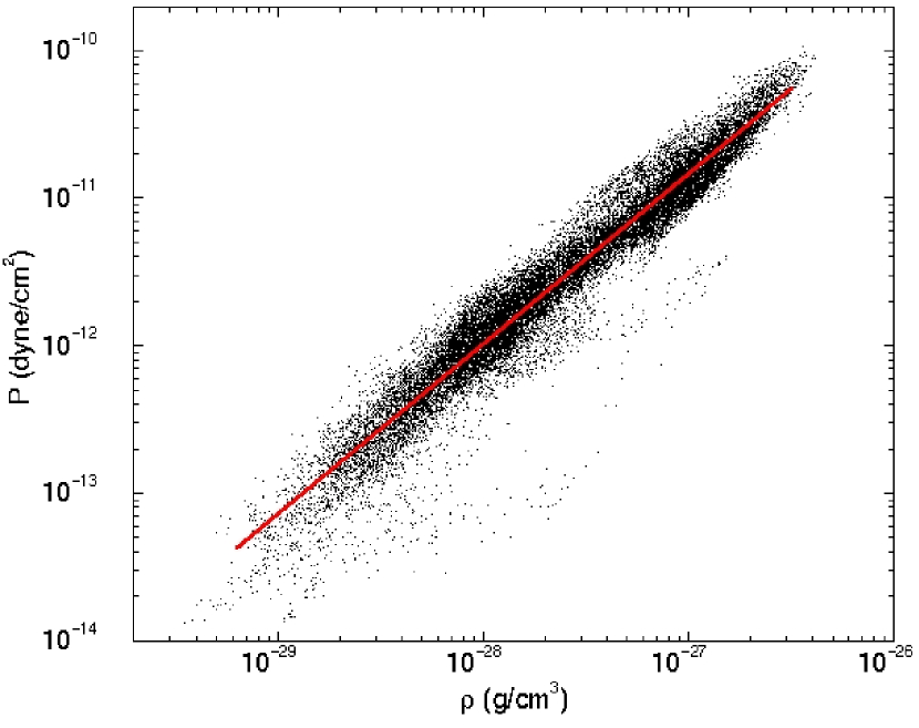
Figure 1: Pressure as a function of density, from an adiabatic simulation of a massive cluster by Greg Bryan. The line has a logarithmic slope of $\Gamma$=1.15.

and the central isothermal gas sound speed is defined as $V^{2}_{s0}={P^{\prime}_{0}}/{\rho^{\prime}_{0}}$. Note that $\Gamma$ is not in fact the actual ratio of specific heats; we require only that the gas has arranged itself in polytropic fashion, as in Eqn. (24). Fig. 1, kindly provided by Greg Bryan, shows results from a high resolution adiabatic AMR simulation of a massive ($\sim 10^{15}h^{-1}M_{\odot}$) cluster. The pressure–density relation in this calculation closely fits that of a $\Gamma=1.15$ polytrope, and lends support for the proposal that turbulent mixing (the only one of the processes listed above that was included in this computation) can lead to a fairly tight polytropic relation. SPH simulations by Lewis et al. (2000) resulted in a pressure-density relation well described by a polytropic equation of state with $\Gamma\approx 1.2$; similar results are reported by Ascasibar et al. (2003) and Borgani et al. (2004). This result holds for both adiabatic and radiative simulations (but see Kay et al., 2004), and agrees well with the effective $\Gamma$ derived from observed clusters by Finoguenov, Reiprich, & Bohringer (2001). Solanes et al. (2005) find that $\Gamma=1.2$ offers the best consistency with the assumption that the specific energy of the hot gas equals that of the dark matter. Interestingly, the purely adiabatic, spherical, and self-similar collapse solution of Bertschinger (1985) was also polytropic with $\Gamma\approx 1.17$.

An additional contribution to the pressure may come from a relativistic component; such a component could be created for example at shock fronts, converting part of the gas energy into cosmic rays. While the relativistic portion of the gas will contain a negligible fraction of the mass, it may contribute significantly to the total gas energy and pressure. We allow for the fact that, in addition to the gas pressure $P^{\prime}$ there may be a nonthermal component having pressure $P_{rel}=\delta_{rel}P^{\prime}$ with total pressure

$$P_{tot} = P^{\prime}+P_{rel}=P^{\prime}(1+\delta_{rel}).$$

It is not obvious if $\delta_{rel}$ is maximum in the center, where there may be injection of a relativistic fluid by an AGN, or in the outer parts of the cluster, where there may be injection of relativistic particle energy in boundary shocks. Thus, for simplicity we will take $\delta_{rel}$ = constant.

Given these relations, the equation of equilibrium for a spherically symmetric distribution, $dP_{tot}/dr=-\rho d\Phi/dr$, becomes

$$(1+\delta_{rel})V^{2}_{s0}\frac{\rho^{\prime}_{0}}{\rho^{\prime}}\frac{d}{dr}\left(\frac{\rho^{\prime}}{\rho^{\prime}_{0}}\right)^{(1+1/n)}=-\frac{GM_{tot}(r)}{r^{2}}\hskip 28.45274pt.$$

Thus

$$\left(\frac{\rho^{\prime}}{\rho^{\prime}_{0}}\right)^{1/n}-1=-\frac{\left[\Phi(r)-\Phi(0)\right]}{V^{2}_{s0}(1+n)(1+\delta_{rel})}=-\frac{\beta j(x)}{(1+n)(1+\delta_{rel})}\hskip 28.45274pt.$$

This last is from Eqn. (4) with

$$\beta\equiv\frac{4\pi G\rho_{1}r_{1}^{2}}{V^{2}_{s0}}=\frac{V_{c,max}^{2}}{V^{2}_{s0}}G_{max}^{-1}$$ (25a)

and

$$j(x)\equiv\left\{\begin{array}[]{ll}1-\frac{\ln(1+x)}{x}&x\leq C\\ 1-\frac{1}{1+C}-\left[\ln(1+C)-\frac{C}{1+C}\right]x^{-1}&x>C\hskip 28.45274pt.\end{array}\right.$$ (25b)

Thus,

$$\rho^{\prime}(r)=\rho^{\prime}_{0}\left[1-\frac{\beta j(x)}{(1+n)(1+\delta_{rel})}\right]^{n}=\rho^{\prime}_{0}\theta^{n}\hskip 28.45274pt,$$ (26a)

where

$$\theta=1-\frac{\beta j(x)}{(1+n)(1+\delta_{rel})}$$ (26b)

is the familiar polytropic variable defined by Chandrasekhar (1967). Eqn. (26a) was first derived by Makino, Sasaki & Suto (1998) for the isothermal case, and Wu, Fabian & Nulsen (2000) more generally. The final gas radius can be smaller or larger than the initial value. Denoting this radius in units of $r_{1}$ as $C_{f}$, the gas mass can be written $M_{g}=4\pi r_{1}^{3}\rho^{\prime}_{0}L$, where

$$L=L(n,\beta,C,C_{f})\equiv\int_{0}^{C_{f}}{\theta^{n}x^{2}dx}\hskip 28.45274pt.$$ (27)

The thermal component will contribute a factor of $\frac{3}{2}\int P^{\prime}d^{3}x$ to the kinetic energy, and the relativistic component $3\int\delta_{rel}P^{\prime}d^{3}x$, so the rearranged total gas energy is $E_{g}^{\prime}=\frac{3}{2}(1+2\delta_{rel})\int_{0}^{M_{g}}{V_{s}^{2}dM}+\int_{0}^{M_{g}}{\Phi_{tot}dM}$. Defining two more integrals

$$I_{2} = I_{2}(n,\beta,C,C_{f})\equiv\int_{0}^{C_{f}}{f(x)\theta^{n}x^{2}dx}$$ (28a)

$$I_{3} = I_{3}(n,\beta,C,C_{f})\equiv\int_{0}^{C_{f}}{\theta^{1+n}x^{2}dx}$$ (28b)

we now have

$$E_{g}^{\prime}=-M_{g}V^{2}_{s0}\left[-\frac{3}{2}(1+2\delta_{rel})\frac{I_{3}}{L}+\beta\frac{I_{2}}{L}\right]$$ (29)

as the final energy.

5 Constraints on the final temperature

Suppose we have a dark matter halo for which the relevant properties— $M_{tot},r_{v},C,V_{c,max}$, etc.— are known. From the previous section, the final distribution of the gas can be determined as a function of the two unknowns $\beta$ and $C_{f}$; thus to specify the final gas temperature and density distribution it remains only to constrain these two parameters. The first constraint is from conservation of energy: the final gas energy will equal the initial energy plus changes to due star formation, expansion or contraction, and feedback; i.e. $E_{g}+\Delta E_{p}+\Delta E_{f}=E_{g}^{\prime}$. Combining this with Eqns. (20), (22), (23), and (29) yields

$$\begin{array}[]{cc}\frac{3}{2}(1+f_{s})\left[G_{max}K(C)\left(3-4\delta_{s}\right)+K_{s}(x_{s})\right]-G_{max}\epsilon f_{s}\frac{c^{2}}{V_{c,max}^{2}}\\ +\frac{1}{3}(1+f_{s})\frac{S_{C}(C)}{g(C)}\left(C^{3}_{f}-C^{3}\right)=\frac{I_{2}}{L}-\frac{3}{2}(1+2\delta_{rel})\frac{I_{3}}{\beta L}\end{array}$$ (30)

(keeping in mind that $L$, $I_{2}$, and $I_{3}$ are functions of $\beta$ and $C_{f}$). A second constraint comes from the fact that the surface pressure of the gas must match the exterior pressure, which we have fixed at $P_{s,gas}(C)$. This gives

$$(1+f_{s})\frac{S_{C}(C)}{g(C)}\beta L=(1+\delta_{rel})\left[1-\frac{\beta j(C_{f})}{(1+n)(1+\delta_{rel})}\right]^{1+n}\hskip 28.45274pt.$$ (31)

Thus, given $r_{v}$, $C$, and $V_{c,max}$ for the dark matter halo, and appropriate choices for $\Gamma$, $f_{s}$, $\epsilon$, and $\delta_{rel}$, Eqns. (30) and (31) can be solved for $\beta$ and $C_{f}$, and the central temperature

$$kT_{0}=\frac{\mu m_{p}}{G_{max}\beta}V^{2}_{c,max}$$ (32)

is known, as is the density parameter $\rho^{\prime}_{0}$, so the gas distribution is fully specified. The expected X-ray luminosity $L_{X}$ can then be calculated. Following Balogh, Babul & Patton (1999), we will include both Bremsstrahlung and recombination, which becomes important for temperatures below 4 keV, by using the cooling function

$$\Lambda(T)=2.1\times 10^{-27}T^{1/2}\left[1+(1.3\times 10^{6}/T)^{3/2}\right]\rm{cm^{3}erg\,s^{-1}.}$$ (33)

5.1 Simulated Halo Catalogue

The plausibility of this procedure can be evaluated by trying it out on a population of many dark matter halos and comparing the results to observed clusters. The halos we use here come from an N-body simulation designed to be in concordance with observational constraints. The simulation is of a periodic cube 1500$h^{-1}$Mpc on a side containing N$=1260^{3}=2\times 10^{9}$ particles. The cosmology was chosen to be a standard LCDM power law model with the following parameters: baryon density $\Omega_{b}=0.047$; Cold Dark Matter density $\Omega_{\rm CDM}=0.223$ (hence total matter density $\Omega_{m}=0.27$); cosmological constant $\Omega_{\Lambda}=0.73$ (thus spatially flat); Hubble constant given by $h=H_{0}/(100{\rm km~{}s^{-1}Mpc^{-1}})=0.70$ (hence $\Omega_{b}h^{2}=0.02303$); primordial scalar spectral index $n_{s}=0.96$; and linear matter power spectrum amplitude $\sigma_{8}=0.84$. These values are consistent within one standard deviation to those derived either from WMAP data or from WMAP combined with smaller angular scale CMB experiments and galaxy data (Spergel et al., 2003). The initial conditions were generated using the publicly available code GRAFIC2 (Bertschinger, 2001) to compute initial particle velocities and displacements from a regular grid. Since the memory required to hold a $1260^{3}$ grid is 8 gigabytes, it was necessary to modify the single level portion of this program by adding message-passing commands in order to distribute the mesh among several processors.

The simulation was carried out with the TPM (Tree-Particle-Mesh) code (Bode & Ostriker, 2003), using 420 processors on the Terascale Computing System at the Pittsburgh Supercomputing Center; it took not quite five days of actual running time. The box size and particle number determine the particle mass of $1.26\times 10^{11}h^{-1}M_{\odot}$. The cubic spline softening length was set to $17h^{-1}$kpc. A standard friends-of-friends (FOF) halo finding routine was run on the redshift $z=0$ box, using a linking length $b=0.2$ times the mean interparticle separation (Lacey & Cole, 1994); this yielded 575,125 halos with both a FOF mass above $2\times 10^{13}h^{-1}M_{\odot}$ and a virial mass above $1.75\times 10^{13}h^{-1}M_{\odot}$. The PM mesh used in TPM contained 1260³ cells, and at redshift zero all PM cells with an overdensity above 39 were being followed at full resolution, so these objects had the full force resolution of TPM. For the range of parameters used here, clusters with $kT>2$keV contained more than 200 particles within $r_{v}$.

For each halo, the position of the most bound particle is taken to be the cluster center. Then $M_{tot}$ and $r_{v}$ are measured, as are $V_{c,max}$ and the radius of maximum circular velocity $r_{c,max}$; this latter gives the concentration $C=2.163r_{v}/r_{c,max}$. This defines the equivalent NFW model halo, i.e. that NFW model closest to the computed dark matter halo. With this information, the procedure outlined above can be carried out on each halo to compute the gas density and temperature.

5.2 Resulting Profiles

Given this set of halos, it remains to specify $\Gamma$, $f_{s}$, $\epsilon$, and $\delta_{rel}$. Let us first consider the appropriate $\Gamma$. Fig. 2 shows the projected temperature profile for different values of $\Gamma$; this profile was computed by integrating the emission-weighted temperature along the line of sight. To normalize the curves, the mean temperature $\langle T\rangle$ was calculated by evenly weighting all radii inside $r_{v}/2$; this was done to correspond with the method of De Grandi & Molendi (2002), who measured the mean profile for clusters with and without cooling flows— shown in the Figure as filled and open circles, respectively. Examination of Fig. 2 shows that $\Gamma$=1.2–1.4, corresponding to polytropes with index $n$=2.5–5, provides adequate fits to the outer parts of the clusters, within which resides most of the gaseous mass (see also the discussion in Solanes et al., 2005). Ascasibar et al. (2003) have shown that a $\Gamma=1.18$ model is a good fit to the average temperature profile measured by Markevitch et al. (1998); this latter measurement has been confirmed by De Grandi & Molendi (2002), Piffaretti et al. (2005), and Vikhlinin, et al. (2005). As discussed above (§4), $\Gamma=1.2$ is also a good fit to hydrodynamical simulations (Lewis et al., 2000; Loken et al., 2002; Ascasibar et al., 2003; Borgani et al., 2004; Kay et al., 2004). The lack of an isothermal core will not lead to a serious overestimation of luminosity or emission-weighted temperature because the volume of this central region is small. This was tested by taking the $\Gamma$=1.2 profile and imposing an isothermal core, matching the density and pressure at $0.2r_{v}$; the resulting changes in emission-weighted temperature and luminosity were generally less than 10%. However, neglecting cooling will reduce the scatter in the $M_{500}-T$ and $L_{x}-T$ relations (McCarthy et al., 2004).

The effect of the polytropic rearrangement on the radial profile of the gas can be seen in Fig. 3. The example halo used here has physical parameters $M_{tot}=4\times 10^{14}h^{-1}M_{\odot}$, $r_{v}=1.2h^{-1}$Mpc, $C=4$, and $V_{c,max}=1200$km/s. The top two panels show the temperature (relative to $T_{ew}$, the mean emission-weighted temperature inside a radius $R_{500}$ containing an density of $500\rho_{c}$) and density (relative to $200\rho_{c}$) as a function of radius. It is instructive to compare to the original NFW distribution, shown as a dot-dashed line; in this case the central temperature goes to zero, as the density profile has a cusp. The polytropic rearrangement (taking $\Gamma=1.2$ and $f_{s}=\epsilon=\delta_{rel}=0$, shown as a dotted line) increases the central temperature while decreasing the density, removing the cusp (with a correspondingly dramatic lowering of the X-ray luminosity, as we shall see). This is seen more clearly in the third panel, which shows the ratio of gas to dark matter mass interior to a given radius, in terms of the cosmic average: inside the dark matter core radius, the gas fraction declines sharply. These temperature and density profiles result in the “entropy” profile shown in the final panel of Fig. 3, taking the definition of entropy to be $T\rho^{-2/3}$. The polytropic profile has a slope close to $r^{1.1}$ near the virial radius, and is shallower nearer the cluster core; this behavior has in fact been observed in a wide range of clusters (Ponman, Sanderson & Finoguenov, 2003; Pratt & Arnaud, 2005; Piffaretti et al., 2005). This behavior has been derived before in analytic models assuming the gas is shock heated (Tozzi & Norman, 2001), and is also seen in hydrodynamic simulations (Lewis et al., 2000; Borgani et al., 2004; Kay et al., 2004).

This change in profile has a strong impact on other observable cluster properties, as is shown in Fig. 4. In these plots the temperature is taken to be the mean emission-weighted $T$ inside $R_{500}$, $T_{ew}$. In clusters with more complicated structure this measure may not coincide well with the spectroscopically measured $T$, as pointed out by Mazzotta et al. (2004), who provide an alternative measure. However, for the simplified models here, the difference between emission weighting and the Mazzotta et al. (2004) spectroscopic-like measure is only a few percent at most. The lines show the median value as a function of $T_{ew}$, found using the dark halo catalogue described in §5.1. The first impact of the polytropic rearrangement is to increase the observed temperatures. This is clearly demonstrated in the left-hand panel, which gives the mass-temperature relation. The points are from Reiprich & Bohringer (2002), as adjusted by McCarthy et al. (2004); here the mass is $M_{500}$, the mass inside a sphere containing mean density 500$\rho_{c}$. The polytropic model distribution (dotted line) resembles that assuming an NFW profile, only shifted to higher $T$; note assuming an NFW gas profile leads to significant disagreement with the observed relation, while switching to a polytropic model provides much superior agreement. This is also true in the right-hand panel, which shows the bolometric X-ray luminosity as a function of $T$; the data points are the subset of the ASCA cluster catalogue (Horner, 2001) described in McCarthy et al. (2004). The polytropic model, without the central cusp, yields a lower luminosity than the NFW profile. The slopes of both the $L_{x}-T$ and $M_{500}-T$ relations retain the same self-similar values, however.

The next physical input is the fraction of gas which collapses into stars. As discussed above, this is roughly one eighth the the gas mass inside the virial radius, or $f_{s}=0.12$. Since the stars in clusters are old, this fraction will hold for all moderately low redshifts. As shown as short-dashed lines in Fig. 3, assuming $f_{s}=0.12$ for a typical cluster (keeping $\Gamma=1.2$) increases the temperature slightly and reduces the gas density. Since the temperature change is not large, this has little effect on the $M_{500}-T$ relation. However, gas removal for star formation, which increases the mean energy per particle for the remaining gas, leads to lower densities and so has a significant impact on the $L_{x}-T$ relation. For the most massive (hottest) clusters, the predicted luminosity is in fact close to that observed; however, the self-similar slope of the relation is still preserved, so for less massive clusters $L_{x}$ is overestimated.

The next required physical input is the amount of energy from feedback coming from supernovae and active galactic nuclei, discussed in §3.2. The results of including feedback of $\epsilon=3.9\times 10^{-5}$ in the $\Gamma=1.2,f_{s}=0.12$ model are shown as long-dashed lines in Figs. 3 and 4. As one would expect, the radial profile has a higher temperature and lower density. However, the effect of feedback differs from those considered previously, because the resulting relations are no longer self-similar. For massive clusters with $V_{c,max}>1000$km/s or $kT>10$keV, feedback is of little importance because the added energy is small compared to the gravitational energy, but for smaller masses it can have a significant impact. One can see a steeper slope in the $M_{500}-T$ relation, but the most significant effect is on the luminosity, which in shape now more closely resembles the observed distribution.

The remaining physical effect left to include is nonthermal pressure. We will take $\delta_{rel}=0.1$; the nonthermal sources of pressure may in fact contribute a few tens of percent of the total (Miniati, 2004). The results can be seen by comparing the solid ($\delta_{rel}=0.1$) and long-dashed ($\delta_{rel}=0$) lines in Figs. 3 and 4. With this additional support, less kinetic energy is required at a given pressure. Thus, while the density profile is little changed, the resulting gas distribution is somewhat cooler, and the emission weighted temperature is lower at a fixed $M_{500}$ or $L_{x}$.

The departure from self-similar scaling is shown further in Fig. 5, which displays the radial profiles of temperature, gas density, gas fraction, and entropy for clusters of mass $M_{tot}=10^{15},5\times 10^{14},2.5\times 10^{14},1.25\times 10^{14}$, and $6.25\times 10^{13}h^{-1}M_{\odot}$. Star formation and feedback were included with $f_{s}=0.12$ and $\epsilon=3.9\times 10^{-5}$, but not a relativistic component. For the least massive cluster we took $C=4$, $V_{c,max}=700$km/s, and $r_{v}=650h^{-1}$kpc, scaling for the others as $C\propto M^{-0.13}$, $V_{c,max}\propto M^{1/3}$, and $r_{v}\propto M^{1/3}$; this is in reasonable agreement with our N-body cluster catalog. With these parameters, the emission weighted temperatures inside $R_{500}$ are $kT_{ew}$=10.1, 6.7, 4.5, 3.1, and 2.2 keV, respectively. For decreasing mass, the temperature and density profiles become increasingly shallow, leading to a faster decrease in X-ray luminosity. The ejection of gas following feedback energy injection leads to a gas fraction (relative to the universal value) less than unity at the virial radius; with the full halo catalog and these parameters we find for halos in the range $1-2\times 10^{14}h^{-1}M_{\odot}$, the gas fraction at the virial radius is $0.72\pm 0.09$ (one standard deviation). This result is in agreement with simulations including both heating and cooling: Muanwong et al. (2002) and Kravtsov, Nagai & Vikhlinin (2005) find that for halos with $M\approx 10^{14}h^{-1}M_{\odot}$ the hot gas fraction inside a radius enclosing overdensity $\approx 100\rho_{c}$ is in the range 0.6–0.7, while Ettori et al. (2004) find slightly higher values of 0.7–0.8. Observational estimates give similar values with a higher scatter (Evrard, 1997; Mohr, Mathiesen & Evrard, 1999; Sanderson & Ponman, 2003). Both these observational and the theoretical studies suggest that more massive clusters have higher hot gas fractions, behavior which is reproduced here.

The bottom panel in Fig. 5 displays the entropy $T/n_{e}^{2/3}$, with $n_{e}$ the electron density in units of cm^-3 (and $T$ in keV), which can be compared directly with the observations listed above. The entropy profiles have a slope close to the observed value of $r^{1.1}$ at the virial radius, but this slope quickly becomes shallower for smaller radii. However, we have not taken into account cooling, which would be more important near the center, steepening the inner entropy profile (McCarthy et al., 2004). It has been observed that the entropy in clusters scales as $T^{0.65}$ (Ponman, Sanderson & Finoguenov, 2003; Pratt & Arnaud, 2005; Piffaretti et al., 2005), rather than linearly in temperature as one would expect for self-similar scaling. Both of these scalings are shown in Fig. 6; the upper panel gives $T/n_{e}^{2/3}/T_{ew}$ and the lower panel $T/n_{e}^{2/3}/T_{ew}^{0.65}$. It is clear from this Figure that the observed $T^{0.65}$ scaling is followed quite closely. However, at radii near $r_{v}$ the observational picture is unclear; with a sample of 14 nearby clusters, Neumann (2005) found that the outer regions followed self-similar scaling and may be affected by the accretion of cooler material. Also, for poorer systems than considered in this paper ($kT<2$keV), we find that this scaling breaks down; such groups may have different entropy profiles than are seen in richer systems (Mahdavi et al., 2005).

6 Generalization to an Arbitrary Dark Matter Potential

The virtue of the method presented in this paper is not just in the equations presented in the preceding sections, whose purpose was to establish physical and mathematical principles and assess the plausibility of the results, but also in its ability to efficiently model complex asymmetrical systems containing substantial substructure. In this section we relax the previous assumption of spherical symmetry and apply the same method to more complex DM potentials. Suppose that a cluster potential is known from an accurate DM integration; the cluster will likely be aspherical and contain significant substructure. Then, if we are satisfied by the ability of an equilibrium polytrope to model the gas in a cluster of galaxies, the integration of the equation of equilibrium $\vec{\nabla}P_{tot}=-\rho\vec{\nabla}\phi$ gives

$$(1+\delta_{rel})\frac{\Gamma}{\Gamma-1}\frac{P(\vec{r})}{\rho(\vec{r})}=-\phi(\vec{r})+(1+\delta_{rel})\frac{\Gamma}{\Gamma-1}\frac{P_{0}}{\rho_{0}}+\phi_{0}\hskip 28.45274pt.$$ (34)

The last two terms comprise a constant of integration; here $\phi_{0}$ is the potential minimum located at position $\vec{r}=\vec{r_{0}}$, and the pressure and density at this point are designated by $P_{0}$ and $\rho_{0}$. Then, making the definition

$$\theta(\vec{r})\equiv 1+\frac{\Gamma-1}{(1+\delta_{rel})\Gamma}\frac{\rho_{0}}{P_{0}}\left(\phi_{0}-\phi(\vec{r})\right)\hskip 28.45274pt,$$ (35)

the pressure and density are simply

$$P(\vec{r})=P_{0}\theta(\vec{r})^{\frac{\Gamma}{\Gamma-1}}$$ (36a)

$$\rho(\vec{r})=\rho_{0}\theta(\vec{r})^{\frac{1}{\Gamma-1}}$$ (36b)

where $\theta(\vec{r})$ is essentially the same polytropic variable defined by Chandrasekhar (1967). Thus for an equilibrium polytropic gas residing in a known potential $\phi(\vec{r})$, the determination of the structure is reduced to the determination of the two numbers $P_{0}$ and $\rho_{0}$. Adopting the approach taken in the previous sections, these constants can be determined by satisfying two equations of constraint on the final energy and the surface pressure.

We carried out this procedure on the same N-body simulation used previously in the following manner. A set of particles identified as a cluster is placed in a nonperiodic 3-D grid. The grid cell size $l$ is set to four times the N-body particle spline softening length, as scales smaller than this can be affected by numerical resolution issues; increasing or decreasing $l$ by a factor of two had little impact on the results. The dark matter density in each cell $k$, $\rho_{k}$, is found from the particle positions using cloud-in-cell (CIC), and the gravitational potential $\phi_{k}$ on the mesh is calculated from the density using a nonperiodic FFT (Hockney & Eastwood, 1981). The position of the cell with the minimum potential $MIN(\phi_{k})=\phi_{0}$ is taken to be the center of the cluster, $\vec{r_{0}}$. The cluster velocity is estimated as the mean velocity of the 125 particles closest to $\vec{r_{0}}$; this mean is subtracted from all the particle velocities. Then the DM kinetic energy per unit volume $t_{k}=\rho v^{2}$ is found in each cell: as with the mass, the kinetic energy of each particle is distributed among 8 cells using CIC. The virial radius $r_{v}$ and DM mass $M_{tot}$ are found from the density distribution. The $N_{cl}$ cells inside $r_{v}$ are identified, as are the $N_{b}$ cells in a buffer region of width $r_{buf}$ surrounding the cluster with centers in the range $r_{v}<r<r_{v}+r_{buf}$. The buffer width was set at 9 cells, or $r_{buf}=153h^{-1}$kpc for the simulation used here. The gas surface pressure is taken to be the mean value (assuming velocities are isotropic) inside this buffer region:

$$P_{s}=N_{b}^{-1}\sum\limits_{k=1}^{N_{b}}\frac{1}{3}\frac{\Omega_{b}}{\Omega_{m}}t_{k}$$ (37)

where the sum is over all cells in the buffer region. Assuming gas traces the DM, the gas mass inside $r_{v}$ is originally $M_{g,i}=\frac{\Omega_{b}}{\Omega_{m}}M_{tot}$. As before, the portion of this gas which is turned into stars is $f_{s}M_{g,i}/(1+f_{s})$. To decide which portion of the gas becomes stars, cells are ranked by binding energy $\rho_{k}\phi_{k}+\text@frac{1}{2}t_{k}$; starting with the most bound cell, the initial $\rho_{k}$ and $t_{k}$ are set to zero for each cell in turn until the gas mass removed, $\frac{\Omega_{b}}{\Omega_{m}}\rho_{k}l^{3}$, totals to $f_{s}M_{g,i}/(1+f_{s})$. The original gas mass inside $r_{v}$ is then

$$M_{g}=\frac{M_{g,i}}{1+f_{s}}=\sum\limits_{k=1}^{N_{cl}}\frac{\Omega_{b}}{\Omega_{m}}\rho_{k}l^{3}$$ (38)

the sum being over all cells inside $r_{v}$, and the initial gas energy is

$$E_{g}=\sum\limits_{k=1}^{N_{cl}}\frac{\Omega_{b}}{\Omega_{m}}\left\{\phi_{k}\rho_{k}+\text@frac{1}{2}t_{k}\right\}l^{3}\hskip 28.45274pt.$$ (39)

As before, this energy can be supplemented by feedback energy $\Delta E_{f}=\epsilon f_{s}M_{g}c^{2}$.

As in the 1-D case, this gas is assumed to rearrange itself into a polytropic distribution with $\Gamma=1.2$. It only remains to specify $P_{0}$ and $\rho_{0}$, which are fixed by the final energy and surface pressure. For a given initial choice of ($P_{0},\rho_{0}$), the final gas density and pressure can be found after calculating $\theta_{k}$ for each cell from Eqn. (35). As before, the initial energy may be changed by the inflow or outflow of gas. The final radius of the gas, $r_{f}$, is found by moving outwards from the cluster center until mass $M_{g}$ is enclosed, i.e.

$$M_{g}=\sum\limits_{k=1}^{N_{f}}\rho_{0}\theta_{k}^{\frac{1}{\Gamma-1}}l^{3}\hskip 28.45274pt,$$ (40)

where the sum is over the $N_{f}$ cells inside $r_{f}$. Similarly to Eqn. (22), we will assume that the surface pressure does not change with radius, so the change in energy due to expansion or contraction is proportional to the change in volume. This means $\Delta E_{P}=(4\pi/3)(r_{v}^{3}-r_{f}^{3})P_{s}$, with $P_{s}$ given by Eqn. (37). Now we have all the information required for the first constraint on ($P_{0},\rho_{0}$), namely the conservation of energy, where the final gas energy is

$$E_{f}=\sum\limits_{k=1}^{N_{cl}}\left\{\rho_{0}\theta_{k}^{\frac{1}{\Gamma-1}}\phi_{0}+\frac{3}{2}P_{0}\theta_{k}^{\frac{\Gamma}{\Gamma-1}}\right\}l^{3}=E_{g}+\Delta E_{f}+\Delta E_{P}\hskip 28.45274pt.$$ (41)

The second constraint is the mean pressure in the $N_{b,f}$ buffer cells between $r_{f}$ and $r_{f}+r_{buf}$; this is assumed to match the original value:

$$N_{b,f}^{-1}\sum\limits_{k=1}^{N_{b,f}}P_{0}\theta_{k}^{\frac{\Gamma}{\Gamma-1}}=P_{s}\hskip 28.45274pt.$$ (42)

Thus after an initial estimate for ($P_{0},\rho_{0}$), it is now possible to iterate to a solution satisfying Eqns. (41) and (42). This solution provides the full three dimensional pressure and density of the gas with allowance for substructure, triaxiality, etc.

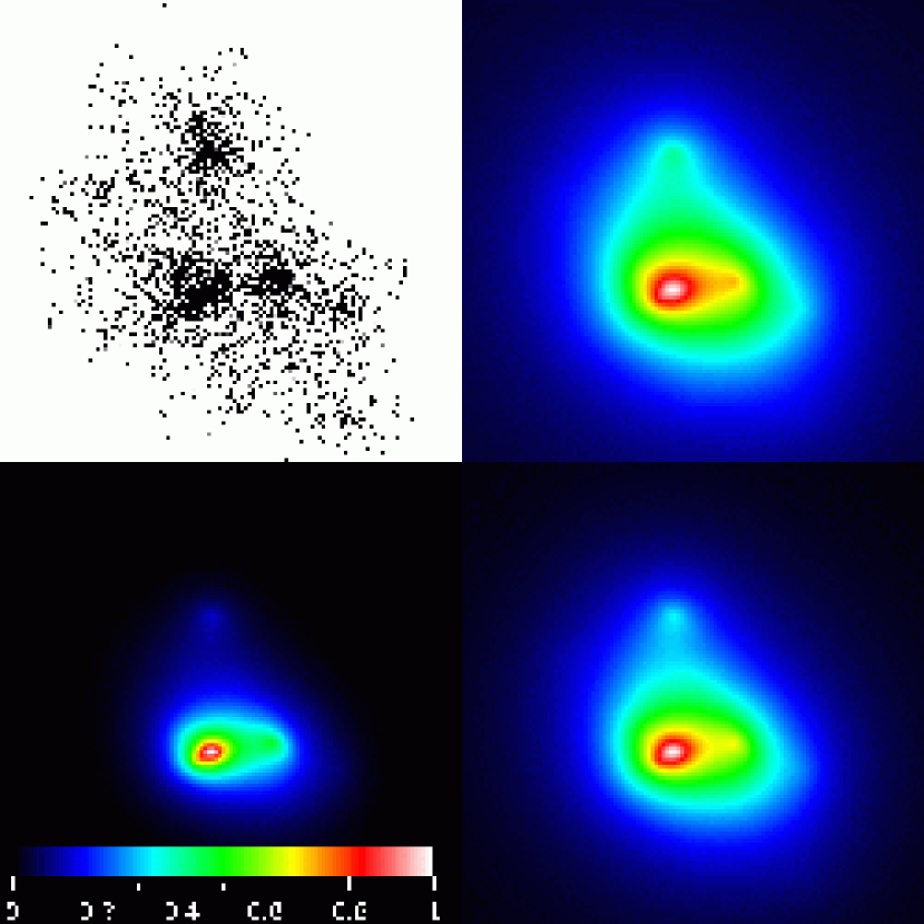
Figure 7: Adding gas to a dark matter halo (drawn from a larger simulation) containing significant substructure. Upper left: DM particle distribution. Upper right: projected gas surface density. Lower left: X-ray luminosity. Lower right: integral of the pressure along the line of sight, proportional to the SZE decrement. The color scale is normalized to the maximum value; the volume shown is 6.4$h^{-1}$Mpc on a side.

An example of the resulting gas distribution for one halo taken from the catalog is given in Fig. 7. The simulation particle positions are shown in the upper left-hand panel; there are several large substructures in the process of merging with the main objects. The volume shown is a cube 6.4$h^{-1}$Mpc on a side. The upper right-hand panel shows the projected gas surface density obtained by the method just described. With the gas density and temperature, maps can be made for the X-ray emission and SZE, as shown in the lower panels. The scale is linear, with black a factor of 100 below white. The results of this procedure employed on the entire set of halos used before are displayed in Fig. 8. A stellar fraction $f_{s}=0.12$ and feedback $\epsilon=3.9\times 10^{-5}$ were included. For each plot, the median value is shown as a solid line and the shaded region encloses 68% of the halos at that temperature. Also shown as dashed lines are the results of the method of §5 based on the NFW profile; the scatter seen using this latter method is somewhat smaller than that shown for the full 3-D method, as the latter realistically includes substructure and triaxiality. We are neglecting cooling, which would increase the scatter further, and tend to increase the luminosity at a given temperature (McCarthy et al., 2004). Use of the NFW approximation appears to have little effect on either the $M_{500}-T$ or the $L_{x}-T$ relation, relative to using the full particle distribution. Examination of individual clusters shows that the spherically averaged gas profiles resulting from the N-body potentials are slightly shallower in both temperature and density, although the amount of gas inside $R_{500}$ is the same for both methods; the larger clumping factor when using the true density, with triaxiality and substructure, increases the luminosity enough to compensate for this.

7 Conclusion

The NFW model has provided a useful description of the distribution of matter inside collisionless DM halos, such as those hosting X-ray clusters. This success inspires hope that a similarly concise description can be found for the hot gaseous component. Given a population of dark matter halos from an N-body simulation (or from some semi-analytic model such as extended Press-Schechter), can we deduce the global properties of the baryonic component inside each halo? In this paper we have worked towards providing a prescription which is simple enough to apply broadly while remaining physically well motivated.

In the model presented here, the gas is assumed to initially have energy per unit mass equivalent to that of the dark matter; this energy can be modified by removal of low entropy gas (to form stars), addition of feedback energy expected from supernovae and accreting black holes, and mechanical work done as the gas expands or contracts. The gas is assumed to redistribute itself into a polytropic distribution in hydrostatic equilibrium with the DM potential; given the constraints on the total energy and the surface pressure at the virial radius, the gas distribution is entirely specified.

We applied two variations of this method to a catalogue of cluster-sized dark matter halos drawn from a large cosmological N-body simulation. In the first variant, the mass, virial radius, and concentration of each halo was measured, and the mass profile was assumed to follow a spherically symmetric NFW profile. To determine the gas distribution in this case means solving Eqns. (30) and (31). We then allowed for complex, nonspherical profiles and substructure by using the full set of particle positions and velocities in each N-body halo to determine the potential and kinetic energy. These two methods give similar results, but assuming a spherical NFW profile gives slightly lower temperatures on average and gives significantly less scatter in the mass-temperature and X-ray luminosity-temperature than is observed.

Simply assuming the gas follows the dark matter leads to too low temperatures and too high central densities, since the DM profile has a cusp. The polytropic rearrangement increases the central temperature while decreasing the density, removing the cusp. Removing low entropy gas for star formation further increases temperatures and reduces density. However, neither of these processes changes the self-similar nature of the model. Including energy from feedback does change this, because in massive clusters the energy input will be small compared to the total binding energy, while for smaller masses it can have more of an impact. We also implemented a simple approximation for including nonthermal pressure support; including a relativistic component in this way leads to somewhat lower temperatures and slightly higher densities.

Essentially two dimensionless numbers are required to prescribe the state of the gas in a given DM potential: the fraction of gas mass transformed to a condensed (primarily stellar) form (determined by observations to have the value $f_{s}\approx 0.12$); and the feedback from the condensed component, for which a plausible estimate for the energy output from supernovae and black holes that is trapped in the cluster gas is $\epsilon f_{s}\approx 0.12\cdot 3.9\times 10^{-5}=4.7\times 10^{-6}$.

The utility of fully understanding the properties of the intergalactic medium in clusters can be seen in Fig. 9, which shows the cumulative temperature function; the data points are from Ikebe et al. (2002). The lines (the line types are the same as in Fig. 3 and Fig. 4) demonstrate how, as different processes are included, the resulting temperature function can change quite dramatically. (Note that the curves are the number density at $z=0$, whereas at the highest $T$ objects are sufficiently rare such that the data points actually reflect the cluster density at $z>0$, which is lower). There is an apparent conflict in that no single model seems to satisfy all the observations simultaneously but this may not be a serious problem, and may in fact reflect the strength of the models. In order to reproduce the observed $M_{500}-T$ and $L_{x}-T$ relations requires a high $T$ and low density, in other words a significant amount of star formation and feedback. But this seems to predict too high a number density of clusters for a given T, as is seen in the plot of $n(>kT)$. However, rather than a problem with the gas model, this may simply be due to our choice of cosmological parameters $\Omega_{m}$ and $\sigma_{8}$ when generating the cluster catalogue. The mass function from our N-body simulation is also too high when compared to that observed by SDSS (see Fig. 2 of Younger, Bahcall & Bode, 2005). Thus an accurate mass-temperature relation would also lead to an overestimate in the temperature function, so the failure to reproduce the observed $n(>kT)$ relation reflects a failure of the cosmological model; lowering $\sigma_{8}$ and/or $\Omega_{m}$ would alleviate this problem without significantly altering the predicted $M_{500}-T$ and $L_{x}-T$ relations. A 10% reduction in $\sigma_{8}$ would reduce the number of clusters with $kT>4$ by roughly a factor of two. This points out the usefulness of the cluster number density as a probe of cosmological parameters, but also the necessity of including all the relevant physics accurately.

A variety of telescopic surveys in many wavelength bands will soon greatly multiply the number of galaxy clusters catalogued, particularly at higher redshifts. Unlocking the power of these new observational datasets as cosmological probes will require sophisticated theoretical predictions. In the future we plan to apply the methods developed here to explore the properties of clusters at higher redshifts and make detailed predictions for X-ray and SZE surveys in many different cosmological models.

Figure 2: Projected temperature profile for $\Gamma=$1, 1.1, 1.2, 1.3, 1.4, and 1.67 (solid lines, from top to bottom at outer radius). $<T>$ is calculated by evenly weighting all radii inside $r_{v}/2$. The points are from De Grandi & Molendi (2002); filled and open circles are clusters with and without cooling flows. The parameters used to calculate the profile are $C=4,V_{c,max}=1200$ km/s, $M_{tot}=4\times 10^{14}h^{-1}M_{\odot}$, and $r_{v}=1.2h^{-1}$Mpc. Aside from the innermost region, the model with a $\Gamma$ of 1.2-1.4 satisfactorily represents the $T$ falloff in the outer regions, which contain most of the gas mass.

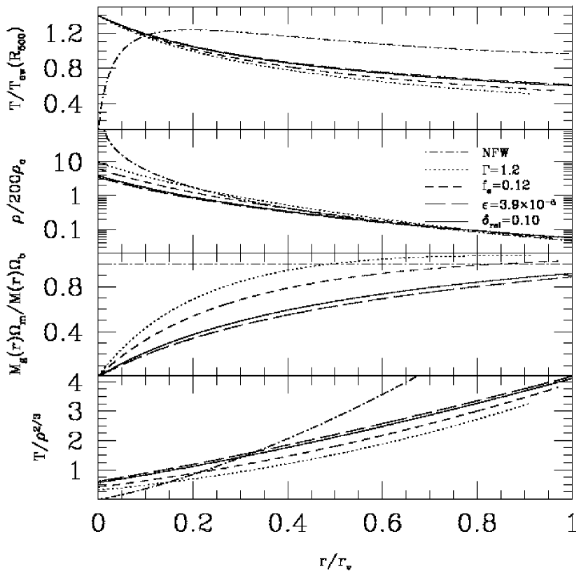
Figure 3: Radial distributions of the temperature, density, mass fraction, and entropy of the gas for different model assumptions. Dot-dashed: gas follows NFW profile. Dotted: hydrostatic equilibrium with polytropic index $\Gamma=1.2$. Short-dashed: also removing 12% of the gas to form stars. Long-dashed: also including energy input from feedback. Solid: also with a relativistic component. In the bottom panel, the entropy is scaled by a factor of $T_{ew}/(200\rho_{c})^{2/3}$.

Figure 4: Results of the model applied to a population of DM halos. Line types as in Fig. 3; lines show the median value as a function of emission-weighted $T$ inside overdensity 500. Left: mass (measured at overdensity 500). Right: bolometric X-ray luminosity. The data points in these two plots are from McCarthy et al. (2004).

Figure 5: Radial distributions for masses $M_{tot}=10^{15},5\times 10^{14},2.5\times 10^{14},1.25\times 10^{14}$, and $6.25\times 10^{13}h^{-1}M_{\odot}$ (line types from top to bottom in uppermost panel). Shown, from top, are temperature, density relative to 200 times critical, the gas mass fraction interior to $r$, and the entropy $T/n_{e}^{2/3}$ (here $n_{e}$ is in units of cm^-3). Parameters used are $\Gamma=1.2$, $f_{s}=0.12$, $\epsilon=3.9\times 10^{-5}$, and $\delta_{rel}=0$.

Figure 6: Radial distribution of entropy $T/n_{e}^{2/3}$ for cluster masses $M_{tot}=10^{15},5\times 10^{14},2.5\times 10^{14},1.25\times 10^{14}$, and $6.25\times 10^{13}h^{-1}M_{\odot}$ (line types as in Fig. 5) scaled by $T_{ew}$ (top panel) and by $T_{ew}^{0.65}$ (bottom panel).

Figure 8: Results from using the directly computed three-dimensional potential of the simulated halos. The solid line in each panel is the median value, and the shaded region encloses 68% of the clusters. The corresponding NFW approximation is shown as a dashed line. Parameters used are $\Gamma=1.2,f_{s}=0.12,\epsilon=3.9\times 10^{-5},$ and $\delta_{rel}=0$. Points are the same as in Fig. 4.

Figure 9: The cumulative temperature distribution function, varying parameters as in Figs. 3 and 4. (using the same line types); data points are from Ikebe et al. (2002). This function will be very sensitive to the choice of cosmological model, particularly $\Omega_{m}$ and $\sigma_{8}$.

References

- Afshordi, Lin & Sanderson (2005) Afshordi, N., Lin, Y-T. & Sanderson, A.J.R. 2005, ApJ, 629, 1
- Allen & Fabian (1998) Allen, S.W. & Fabian, A.C. 1998, MNRAS, 297, L57
- Ascasibar et al. (2003) Ascasibar, Y., Yepes, G., Mueller, V. & Gottloeber, S. 2004, MNRAS, 346, 731
- Avila-Reese et al. (1999) Avila-Reese, V., Firmani, C., Klypin, A. & Kravtsov, A.V. 1999, MNRAS, 310, 527
- Babul et al. (2002) Babul, A., Balogh, M.L., Lewis, G.F. & Poole, G.B. 2002, MNRAS, 330, 329
- Balogh, Babul & Patton (1999) Balogh, M.L., Babul, A. & Patton, D.R. 1999, MNRAS, 307, 463
- Balogh et al. (2001) Balogh, M.L., Pearce, F.R., Bower, R.G. & Kay, S.T. 2001, MNRAS, 326, 1228
- Bertschinger (1985) Bertschinger, E. 1985, ApJS, 58, 39
- Bertschinger (2001) Bertschinger, E. 2001, ApJS, 137, 1
- Bode & Ostriker (2003) Bode, P. & Ostriker, J.P. 2003, ApJS, 145, 1
- Borgani et al. (2004) Borgani, S., Murante, G., Springel, V., Diaferio, A., Dolag, K., Moscardini, L., Tormen, G., Tornatore, L. & Tozzi, P. 2004, MNRAS, 348, 1078
- Bower et al. (2001) Bower, R.G., Benson, A.J., Lacey, C.G., Baugh, C.M., Cole, S. & Frenk, C.S. 2001, MNRAS, 325, 497
- Bryan & Norman (1998) Bryan, G.L. & Norman, M.L. 1998, ApJ, 495, 80
- Bryan & Voit (2005) Bryan, G.L. & Voit, G.M. 2005, Phil. Trans. R. Soc. A, 363, 715
- Bullock et al. (2001) Bullock, J.S., Kolatt, T.S., Sigad, Y., Somerville, R.S., Kravtsov, A.V., Klypin, A.A., Primack, J.R., & Dekel, A. 2001, MNRAS, 321, 559
- Bykov (2005) Bykov, A.M. 2005, Advances in Space Research, in press (astro-ph/0501575)
- Carilli & Taylor (2002) Carilli, C.L. & Taylor, G.B. 2002, ARA&A, 40, 319
- Cen (2005) Cen, R., 2005, ApJ, 620, 191
- Chandrasekhar (1967) Chandrasekhar, S. 1967, An Introduction to the Study of Stellar Structure, New York: Dover, 86
- De Grandi & Molendi (2002) De Grandi, S. & Molendi, S. 2002, ApJ, 567, 163
- Dos Santos & Doré (2002) Dos Santos, S. & Doré, O. 2002, A&A, 450
- Dolag et al. (2004) Dolag, K., Jubelgas, M., Springel, V., Borgani, S. & Rasia, E. 2004, ApJ, 606, L97
- Edge & Stewart (1991) Edge, A.C. & Stewart, G.C. 1991, MNRAS, 252, 414
- El-Zant, Kim & Kamionkowski (2004) El-Zant, A., Woong-Tae Kim, W-T. & Kamionkowski, M. 2004, MNRAS, 354, 169
- Ensslin, Vogt & Pfrommer (2005) Ensslin, T.A., Vogt, C. & Pfrommer, C. 2005, Proceedings of the workshop ”The Magnetized Plasma in Galaxy Evolution”, K.T. Chyzy, R.-J. Dettmar, K. Otmianowska-Mazur, & M. Soida, Krakow:Jagiellonian University (astro-ph/0501338)
- Ettori et al. (2004) Ettori, S., Borgani, S., Moscardini, L., Murante, G., Tozzi, P., Diaferio, A., Dolag, K., Springel, V., Tormen, G. & Tornatore, L. 2004, MNRAS, 354, 111
- Evrard (1997) Evrard, G. 1997, MNRAS, 292, 289
- Faltenbacher et al. (2004) Faltenbacher, A., Kravtsov, A.V., Nagai, D. & Gottloeber, S. 2004, MNRAS, 358, 139
- Finoguenov, Reiprich, & Bohringer (2001) Finoguenov, A., Reiprich, T.H. & Bohringer, H. 2001, A&A, 368, 749
- Frenk et al. (1999) Frenk, C.S., et al. 1999, ApJ, 525, 554
- Fukugita, Hogan & Peebles (1998) Fukugita, M., Hogan, C.J. & Peebles, P.J.E. 1998, ApJ, 503, 518
- Fukushige, Kawai & Makino (2004) Fukushige, T., Kawai, A. & Makino, J. 2004, ApJ, 606, 625
- Hockney & Eastwood (1981) Hockney, R.W. & Eastwood, J.W. 1981, Computer Simulation Using Particles, New York:McGraw-Hill
- Horner (2001) Horner, D.J. 2001, Ph.D. Thesis, University of Maryland
- Ikebe et al. (2002) Ikebe, Y., Reiprich, T.H., Bohringer, H., Tanaka, Y. & Kitayama, T. 2002, A&A, 383, 773
- Inoue & Sasaki (2001) Inoue,S. & Sasaki, S. 2001, ApJ, 562, 618
- Jing (2000) Jing, Y.P. 2000, ApJ, 535, 30
- Kaiser (1986) Kaiser, N. 1986, MNRAS, 222, 323
- Kaiser (1991) Kaiser, N. 2001, ApJ, 383, 104
- Kay et al. (2004) Kay, S.T., Thomas, P.A., Jenkins, A. & Pearce, F.R. 2004, MNRAS, 355, 1091
- Kim & Narayan (2003a) Kim, W-T. & Narayan, R. 2003, ApJ, 596, 889
- Kim & Narayan (2003b) Kim, W-T. & Narayan, R. 2003, ApJ, 596, L139
- Klypin et al. (2001) Klypin, A., Kravtsov, A., Bullock, J. & Primack, J. 2001, ApJ, 554, 903
- Komatsu & Seljak (2001) Komatsu, E., & Seljak, U. 2001, MNRAS, 327, 1353
- Kormendy & Gebhardt (2000) Kormendy, J., & Gebhardt, K. 2000, AIP Conf. Proc. 586, 20th Texas Symp. on Relativistic Astrophysics, ed. J.C. Wheeler & H. Martel (New York: AIP), 363
- Kravtsov, Nagai & Vikhlinin (2005) Kravtsov, A.V., Nagai, D. & Vikhlinin, A.A. 2005, ApJ, submitted (astro-ph/0501227)
- Lacey & Cole (1994) Lacey, C. & Cole, S. 1994, MNRAS, 271, 676
- Lapi, Cavaliere & Menci (2005) Lapi, A., Cavaliere, A. & Menci, N. 2004, ApJ, 619, 60
- Lewis et al. (2000) Lewis, G.F., Babul, A., Katz, N., Quinn, T., Hernquist, L. & Weinberg, D.H. 2000, ApJ, 536, 623
- Lin, Mohr & Stanford (2003) Lin, Y-T., Mohr, J.J. & Stanford, S.A. 2003, ApJ, 591, 749
- Lokas & Mamon (2001) Lokas, E.W, & Mamon, G.A. 2001, MNRAS, 321, 155
- Loken et al. (2002) Loken, M., Norman, M.L., Nelson, E., Burns, J., Bryan, G.L. & Motl, P. 2002, ApJ, 579, 571
- Mahdavi et al. (2005) Mahdavi, A., Finoguenov, A., Bohringer, H., Geller, M.J. & Henry, J.P. 2005, ApJ, 622, 187
- Makino, Sasaki & Suto (1998) Makino, N., Sasaki, S. & Suto, Y. 1998, ApJ, 497, 555
- Markevitch (1998) Markevitch, M. 1998, ApJ, 504, 27
- Markevitch et al. (1998) Markevitch, M., Forman, W.R., Sarazin, C.L. & Vikhlinin, A. 1998, ApJ, 503, 77
- Mazzotta et al. (2004) Mazzotta, P., Rasia, E., Moscardini, L. & Tormen, G. 2004, MNRAS, 354, 10
- McCarthy et al. (2004) McCarthy, I.G., Balogh, M.L., Babul, A., Poole, G.B. & Horner, D.J. 2004, ApJ, 613, 811
- Merrit & Ferrarese (2001) Merrit, D. & Ferrarese, L. 2001, MNRAS, 320, L30
- Miniati (2004) Miniati, F. 2004, Modelling the Intergalactic and Intracluster Media, ed. V. Antonuccio-Delogu (astro-ph/0401480)
- Mohr, Mathiesen & Evrard (1999) Mohr, J. Mathiesen, B. & Evrard, G. 1999, ApJ, 517, 627
- Muanwong et al. (2002) Muanwong, O., Thomas, P.A., Kay, S.T. & Pearce, F.R. 2002, 336, 527
- Norman & Bryan (1999) Norman, M.L. & Bryan, G.L. 1999, The radio galaxy Messier 87 (Lecture notes in physics 530), H.-J. Roeser & K. Meisenheimer, New York:Springer, 106