Iron abundances derived from RR Lyrae light curves and low-dispersion spectroscopy

With the aid of the All Sky Automated Survey (ASAS) database on the Galactic field, we compare the iron abundances of fundamental mode RR Lyrae stars derived from the Fourier parameters with those obtained from low-dispersion spectroscopy. We show from a set of 79 stars, distinct from the original calibrating sample of the Fourier method and selected without quality control, that almost all discrepant estimates are the results of some defects or peculiarities either in the photometry or in the spectroscopy. Omitting objects deviating by more than $0.4$ dex, the remaining subsample of 64 stars yields Fourier abundances that fit the spectroscopic ones with $\sigma=0.20$ dex. Other, more stringent selection criteria and different Fourier decompositions lead to smaller subsamples and concomitant better agreement, down to $\sigma=0.16$ dex. Except perhaps for two variables among the 163 stars, comprised of the ASAS variables and those of the original calibrating set of the Fourier method, all discrepant values can be accounted for by observational noise and insufficient data coverage. We suggest that the agreement can be further improved when new, more accurate spectroscopic data become available for a test with the best photometric data. As a by-product of this analysis, we also compute revised periods and select Blazhko variables.

1 Introduction

Determination of the chemical composition of RR Lyrae stars is an important task because of the general astrophysical relevance of these objects. Unfortunately, RR Lyrae stars have low brightness, and therefore most of them are accessible for more thorough spectroscopic investigations only by large telescopes. Furthermore, due to large variations in effective surface gravity and temperature during the pulsation, complicated hydrodynamical phenomena (moving ionization fronts and shocks) take place on time scales of an hour, which make the observations and analysis more difficult. For these reasons, high dispersion spectroscopic observations of RR Lyrae stars are rather rare (see Butler et al. 1982; Clementini et al. 1994, 1995; Fernley & Barnes 1996; Lambert et al. 1996; Sandstrom, Pilachowski & Saha 2001), and aimed partially at the calibration of some variants of the spectral index method originally devised by Preston (1959). The overwhelming majority of the information available for us on the heavy abundance of RR Lyrae stars comes from these spectral index methods.

Although the acquisition of low-dispersion spectroscopic data is easier than that of high-dispersion data, with the increasing demand for studying more distant objects in dense stellar clusters and galaxies, the question arose of whether the more easily accessible light curves could be used for metallicity estimation. The fact that the period, amplitude and metallicity are correlated has been known since the pioneering paper of Preston (1959). However, the accuracy and the amount of the then-available data did not allow him to recognize the existence of a tighter correlation with another parameter associated with the shape of the light curve. By using accurate photometric and low-dispersion spectroscopic data, it was found that a simple linear formula, employing the period $P$ and the Fourier phase $\varphi_{31}$, correlates very well with the observed [Fe/H] and is able to predict the measured values with a standard deviation of $0.13$ dex (Jurcsik & Kovács 1996, hereafter JK96).

Because of the accurate fit of the Fourier formula to the observed metallicities of the fundamental mode (RRab) field stars, it would be very attractive to use it on various large databases. Before one pursues such a task, it is useful to test the reliability of the method on various independent datasets with known metallicities. Several attempts have been made in this direction during the past several years. The first one was that of JK96 who compared globular cluster metallicities derived from the spectroscopy of giants with those computed by the Fourier method on the RRab stars of the respective clusters. The conclusion was that the overall agreement was satisfactory, but there was a hint that at the low-metallicity end the Fourier method gave somewhat higher values. Schwarzenberg-Czerny & Kaluzny (1998) examined the correlation of the individual low-dispersion metallicities obtained by Butler, Dickens & Epps (1978) for $\omega$ Cen. They concluded that the expected correlation was not seen. Subsequently, for the same cluster, Rey et al. (2000) found a correlation with the Fourier data when using metallicities derived from their Caby photometry. Borissova et al. (2004) compared the metallicities of a few stars in $\omega$ Cen derived from their modified $\Delta S$ method (adopted from Layden 1994, hereafter L94) with those obtained by Butler et al. (1987) and by Rey et al. (2000). They found that the former ones (used also by Schwarzenberg-Czerny & Kaluzny 1998) were in better agreement with theirs than the latter ones. For M3, Jurcsik (2003) argued that the correlation of the direct spectroscopic observations of Sandstrom et al. (2001) with the ones derived by the Fourier method was significant, suggesting a real metallicity spread in this globular cluster. Based on a current sample of 22 RRab stars with low-dispersion spectroscopic abundances in the Large Magellanic Cloud (LMC), Gratton et al. (2004) concluded that, after selecting outliers, the derived standard deviation of $0.24$ dex between the Fourier and spectroscopic abundances were in agreement with the errors of the measurements.

All these suggest that in spite of the various efforts to accumulate new spectroscopic abundances for RR Lyrae stars, the accuracy and the amount of the data used in the above tests are insufficient to draw a firm conclusion on the reliability of the Fourier method. Unfortunately, there are no current large-scale low-dispersion surveys available and there is also a lack of similar undertakings on the high-dispersion side. There is also a need for extended multicolor photometry. Except for the current releases of photometric time series by the All Sky Automated Survey (ASAS) and the Robotic Optical Transient Search Experiment (ROTSE) projects (see Pojmanski 2002, 2003, Pojmanski & Maciejewski 2004, Wozniak et al. 2004) and perhaps for the Behlen Observatory survey (Schmidt & Seth 1996) and that of Layden (1997), no significant efforts have been made to extend the photometric database for Galactic field RR Lyrae stars since the formula of JK96 was derived.

For a useful test of the Fourier formula, we need reliable light curves observed in Johnson $V$ band, with corresponding [Fe/H] values either from L94 or from Suntzeff, Kraft & Kinman (1994, hereafter S94). (We recall that it was shown by JK96 that the two databases are statistically equivalent.) Various reasons (no $V$ band observations by ROTSE, few data points per star in the Behlen survey, too few variables with proper light curves and overlaps with the ASAS database in the survey of Layden 1997) led us to utilize only the database of the ASAS survey. Although we think that this database, combined with the metallicities of L94, constitutes the most stringent current test, it is important to keep in mind its limitations. Most importantly, many of the variables are rather faint and therefore, due to the small aperture telescopes employed by the ASAS project, they exhibit relatively large scatter (compensated partially by the large number of data points per star). In addition, no time-dependent color term was employed in the transformation to the standard magnitude system, therefore, small distortions of the published light curves are expected. The fainter objects used in our tests are also more likely to show larger errors in their measured metallicities. Nevertheless, as it is shown later, the present test supports the applicability of the Fourier method in the determination of the iron abundances of RRab stars.

2 Light curves and metallicities

Table 1: ASAS variables common with those in the compilation of JK96

Variable	Period [d]	[Fe/H]	Rem	Variable	Period [d]	[Fe/H]	Rem	Variable	Period [d]	[Fe/H]	Rem
WY Ant	0.574341	$-1.39$	1D	SV Hya	0.478548	$-1.43$	BL	TY Pav	0.710382	$-2.01$	$-$
V Cae	0.570914	$-1.71$	$-$	DH Hya	0.489002	$-1.28$	$-$	U Pic	0.440375	$-0.50$	1D
IU Car	0.737059	$-1.57$	LD	FY Hya	0.636650	$-2.03$	$-$	RY Psc	0.529746	$-1.18$	BL
V499 Cen	0.521212	$-1.29$	1D	SS Leo	0.626337	$-1.56$	$-$	BB Pup	0.480549	$-0.35$	LD
RR Cet	0.553028	$-1.29$	$-$	TV Leo	0.672860	$-1.86$	$-$	AV Ser	0.487563	$-0.95$	$-$
RX Cet	0.573727	$-1.20$	BL	U Lep	0.581479	$-1.67$	$-$	RW Tra	0.374039	$0.27$	$-$
RZ Cet	0.510600	$-1.24$	BL	TV Lib	0.269623	$-0.17$	$-$	W Tuc	0.642236	$-1.37$	$-$
W Crt	0.412013	$-0.45$	$-$	VY Lib	0.533940	$-1.06$	$-$	UU Vir	0.475608	$-0.60$	$-$
RX Eri	0.587247	$-1.07$	$-$	RV Oct	0.571170	$-1.08$	1D	AT Vir	0.525777	$-1.54$	$-$
BB Eri	0.569910	$-1.23$	LD	ST Oph	0.450356	$-1.02$	$-$	$-$	$-$	$-$	$-$
SX For	0.605342	$-1.35$	$-$	V445 Oph	0.397023	$0.01$	$-$	$-$	$-$	$-$	$-$

Notes: $\rm[Fe/H]$ : spectroscopic iron abundance as given in JK96; BL : Blazhko variable; 1D : light curve is affected by an instrumental effect of $n$d^-1 frequency ($n=1,2,...$); LD : long-term drift or periodic variation in the average light level

Table 2: ASAS variables separate from those in the compilation of JK96

Variable	Period [d]	[Fe/H]	Rem	Variable	Period [d]	[Fe/H]	Rem	Variable	Period [d]	[Fe/H]	Rem
TY Aps	0.501699	$-0.96$	1D	SW Dor	0.525338	$-1.33$	$-$	UV Oct	0.542582	$-1.34$	BL
UY Aps	0.482513	$-0.45$	$-$	SX Dor	0.631449	$-1.71$	$-$	AR Oct	0.394029	$-0.29$	LD
VX Aps	0.484665	$-1.18$	BL	VW Dor	0.570569	$-0.99$	BL	V413 Oph	0.449001	$-0.76$	$-$
XZ Aps	0.587268	$-1.30$	1D	XY Eri	0.554272	$-1.79$	BL	V1023 Oph	0.623930	$-0.96$	1D
AR Aps	0.610717	$-1.49$	$-$	BK Eri	0.548165	$-1.37$	$-$	WY Pav	0.588572	$-0.74$	1D
BS Aps	0.582561	$-1.33$	1D	AC Eri	0.482083	$-1.06$	$-$	TZ Phe	0.615603	$-1.04$	$-$
CK Aps	0.623631	$-1.23$	BL	AL Eri	0.656941	$-1.61$	BL	HH Pup	0.390746	$-0.46$	$-$
DD Aps	0.648108	$-0.81$	$-$	RX For	0.597317	$-1.01$	BL	X Ret	0.492016	$-1.06$	BL
DI Aps	0.519180	$-1.33$	$-$	SS For	0.495434	$-1.09$	BL	V765 Sco	0.463662	$-0.93$	$-$
EL Aps	0.579722	$-1.29$	$-$	SW For	0.803760	$-1.67$	$-$	RU Scl	0.493356	$-1.00$	$-$
ER Aps	0.758417	$-1.13$	$-$	UU Hor	0.643691	$-1.52$	$-$	VX Scl	0.637047	$-1.95$	$-$
EX Aps	0.471801	$-0.58$	1D	SZ Hya	0.537228	$-1.48$	BL	WY Scl	0.463685	$-1.25$	$-$
LU Aps	0.755038	$-1.77$	$-$	WZ Hya	0.537718	$-1.04$	$-$	AE Scl	0.550113	$-1.61$	$-$
U Cae	0.419782	$-0.86$	$-$	XX Hya	0.507752	$-1.07$	$-$	RV Sex	0.503417	$-0.85$	BL
KS Cen	0.397445	$-0.57$	$-$	DG Hya	0.754242	$-1.16$	$-$	AE Tuc	0.414529	$-0.57$	1D
V671 Cen	0.779058	$-1.14$	$-$	ET Hya	0.685521	$-1.42$	$-$	AG Tuc	0.602584	$-1.67$	$-$
V674 Cen	0.493935	$-1.26$	1D	FX Hya	0.417338	$-0.83$	$-$	BK Tuc	0.550068	$-1.54$	$-$
UU Cet	0.606073	$-1.74$	$-$	GS Hya	0.522831	$-1.48$	BL	FS Vel	0.475754	$-0.92$	$-$
RU Cet	0.586284	$-1.33$	BL	IV Hya	0.532251	$-1.08$	$-$	ST Vir	0.410813	$-0.64$	$-$
RV Cet	0.623410	$-1.06$	BL	TW Hyi	0.675383	$-1.39$	$-$	UV Vir	0.587084	$-0.94$	$-$
RV Cha	0.701400	$-1.39$	$-$	XX Lib	0.698452	$-1.21$	1D	WW Vir	0.651559	$-1.84$	$-$
RT Col	0.536580	$-1.17$	$-$	T Men	0.409820	$-0.61$	$-$	AM Vir	0.615083	$-1.19$	BL
RW Col	0.545615	$-0.79$	$-$	RX Men	0.456290	$-1.27$	1D	AS Vir	0.553436	$-1.23$	$-$
RX Col	0.593766	$-1.43$	BL	EM Mus	0.467286	$-1.28$	$-$	BQ Vir	0.637029	$-1.06$	BL
RY Col	0.478840	$-0.86$	BL	Y Oct	0.646571	$-1.26$	1D	SV Vol	0.609919	$-1.89$	BL
X Crt	0.732835	$-1.48$	BL	RS Oct	0.457999	$-1.33$	BL	$-$	$-$	$-$	$-$
RT Dor	0.482834	$-1.26$	$-$	SS Oct	0.621850	$-1.33$	BL	$-$	$-$	$-$	$-$

Notes: $\rm[Fe/H]$ : Spectroscopic iron abundance as given in Layden (1994) or in Suntzeff et al. (1994); BL, 1D, LD : as in Table 1

In 2004 the ASAS project completed the variability survey of the $0^{\rm h}-18^{\rm h}$ segment of the southern hemisphere. Among the many other variables, they classified 723 RRab stars. All light curves contain some 100–700 data points. We searched the ASAS web site for RRab variables found also in the [Fe/H] catalogs of L94 or S94. We found 110 variables satisfying this criterion. The data cover a period of 3.7 y, giving an ample timebase for the analysis of the stability of the light variation. For each variable, the database contains five time series, corresponding to five different aperture sizes used in the photometry. All variables have been subjected to an analysis consisting of the following steps.

• Time series $V(t)$ were generated through the weighted average of the magnitude values $V_{i}(t)$ given for the five apertures. By using the assigned standard deviations $\sigma_{i}(t)$, we have

  $$V(t) = \sum_{i=1}^{5}V_{i}(t)\sigma^{-2}_{i}(t)\over{\sum_{i=1}^{5}\sigma^{-2}_{i}(t)}$$

• Frequency analysis of $V(t)$ was performed in the [0,3] d^-1 interval, searched for the best period with a non-linear least squares method and thereafter prewhitened in order to find possible additional components. We employed the time series analysis program package mufran (Kolláth, 1990)

• In order to avoid overfitting noisy light curves and underfitting those with low noise, after manual experiments, we use the following condition on the order of the Fourier fit. For each aperture, the light curve was fitted by a Fourier sum of order $m$, computed from the following condition

  $$m=\left\{\begin{array}[]{ll}4&\mbox{if $m^{\star}<4$}\\ $$m^{\star}$$&\mbox{if $4\leq m^{\star}\leq 10$}\\ 10&\mbox{if $m^{\star}>10$}\end{array}\right.$$

  Here the ‘empirical’ order $m^{\star}$ is given by $m^{\star}=INT({\rm SNR}/10)$, where the symbol $INT$ stands for the integer part and the the signal-to-noise ratio. The latter quantity is computed by

  $${\rm SNR} = A_{1}\sqrt{n}/\sigma$$

  where $A_{1}$ is the Fourier amplitude at the main frequency component, $n$ is the number of data points and $\sigma$ is the standard deviation of the residuals between the data and the fit.

• Outliers were discarded at the $3\sigma$ level and the Fourier fit was repeated until no outliers were found.

• Finally we stored the light curve corresponding to that aperture size which yielded the highest SNR.

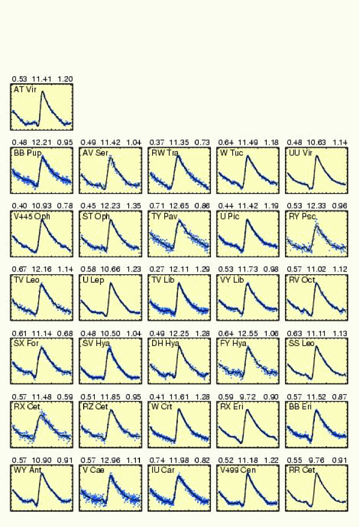
Figure 1: Folded light curves from the ASAS database. All variables enter also in the compilation of JK96. Headers: period [d], average brightness in $V$ and total amplitude [mag] of the fitted light curve (continuous line). The orders of the Fourier fits were determined from the SNR of the light curves as described in the text. All light curves were obtained in Johnson $V$ color. With centered peak brightness, the light curves are plotted in the $1.5$ phase interval.

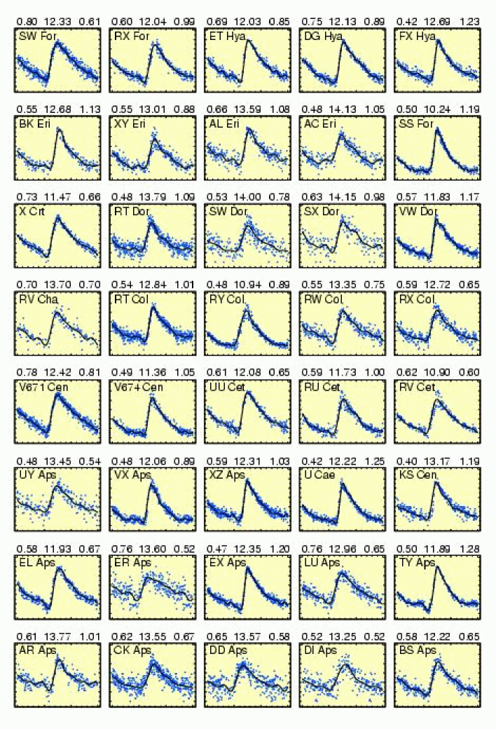
Figure 2: Folded light curves from the ASAS database. None of the variables enter in the compilation of JK96 but all have low-dispersion spectroscopic metallicities either from Layden (1994) or from Suntzeff et al. (1994). Notation is the same as in Fig. 1.

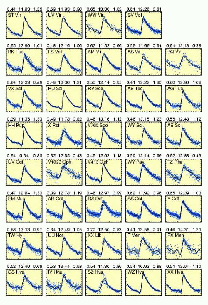
Figure 3: Folded light curves from the ASAS database. Data selection and notation are the same as in Fig. 2.

The set of 110 variables is separated into two groups. The first group (set #1, with 31 stars) is common with a subset of the variables used by JK96. This set is used primarily to compare the ASAS photometry with the one of JK96, that is based on traditional photometric observations of various origins. The second group (set #2, with 79 stars) has no common members with the dataset of JK96. This set is used to check the predictive power of the Fourier formula for [Fe/H]. Variable names, derived periods (based on the ASAS database), iron abundances and comments on the light variations of the individual variables are listed in Tables 1 and 2 for sets #1 and #2, respectively. Folded light curves with the corresponding Fourier fits are displayed in Figs. 1, 2 and 3.

Iron abundances in Table 1 are the same as given in JK96. We recall that except for two stars among the 84 variables entering in the compilation of JK96, all abundances were computed from the weighted and zero-point-shifted averages of S94 and L94. The metallicity scale of Jurcsik (1995) is used that corresponds to the scale of the high-dispersion spectroscopic studies and is similar to those of Clementini et al. (1995) and Lambert et al. (1996), with these latter calibrations being more metal-poor by 0.1–0.15 dex. The abundances in Table 2 were obtained almost exclusively from L94. For UU Cet and AL Eri we utilized the data of S94.

The frequency analysis (combined with prewhitening) allowed us to identify a number of Blazhko (BL) variables, together with those showing integer d^-1 periodicities in the prewhitened spectra (1D stars) and with those displaying long-periodic variations in their average light levels (LD stars). Due to aliasing, in some cases ambiguity might exist between the 1D and LD classifications. Except perhaps for a few cases, these variations are thought to be related to some anomaly in the method employed in the data reduction pipeline. These types of systematics are common in almost all photometric databases, but especially in the ones originating from wide field photometry (see Kovács, Bakos & Noyes 2005 and references therein).

Classification of the BL stars was based on the occurrence of nearby component(s) at the fundamental pulsation frequency. We found 26 BL variables from the 110 RRab stars. Most of these are new discoveries, some of them (e.g., RU~Cet, SV~Vol) show weak, whereas others (e.g., RX~Cet, SZ~Hya) show strong Blazhko effects. The derived incidence rate of 24% is in agreement with the one found by Moskalik & Poretti (2003) from the analysis of 150 RRab stars in the Galactic bulge and also in line with the earlier quoted rates for RRab stars in general (Szeidl 1988). The above rate for the LMC is only 12% (Alcock et al. 2003), and it is tempting to attribute this lower value to the lower average metallicity of the LMC. Nevertheless, by checking the entries in our tables, it seems to us that one cannot draw such a simple conclusion, since both low- and high-metallicity stars can be found among the Galactic field BL variables.

By inspecting the folded light curves, we see that most of them are of good or fine quality, in spite of the expected large scatter at these faint magnitudes for photometric data obtained by a small-aperture telescope. Some of the fainter variables display rather large scatter due to observational noise. We left these stars in the sample, in order to test cases when the observational noise is more considerable, such as in the microlensing surveys of the Magellanic Clouds. A more thorough comparison of the set #1 light curves will follow in the next subsection. Concerning set # 2, we made a comparison with the periods published at the ASAS homepage. In general, we found that the periods agreed within $2\times 10^{-5}$ d. In several instances our periods yielded better representations of the data (e.g., V674~Cen, SS~For, VX~Scl).

The overall performance of the SNR-dependent Fourier fit is acceptable, but we see signatures of artifacts in some cases. These artifacts appear as unphysical waves and are related to as insufficient number of data points, sharp light curve variations or non-uniform coverage of the folded light curve. Some aspects of these sampling problems can be handled by the polynomial fitting method mentioned in JK96. In the present case this method performed slightly worse, i.e., yielded a few additional outliers in the comparison of the spectroscopic and Fourier metallicities. Therefore, we use the straightforward SNR-dependent Fourier fit, although in many cases the differences are small, mostly induced by noise.

2.1 Comparison with the compilation of JK96

Here, and in all subsequent comparisons of various datasets we follow a two-step procedure: (i) comparison of all available stars, disregarding any suspected source of defects (e.g., noise, systematics) or peculiarities (e.g., Blazhko effect); (ii) select outliers, check the agreement with the remaining sample and investigate the possible source(s) of discrepancy. This procedure likely leaves some stars in the sample that would otherwise be discarded. Nevertheless, we prefer this approach over the one followed by JK96, because the pre-selection procedure we applied there led to the omission of objects that otherwise fitted the calibration sample. In Sect. 3 we discuss other outlier selection strategies and the results obtained by their application.

Before making a more thorough comparison, we show two examples to display the range of differences between the two datasets. In Fig. 4 we display the type of agreement we have for about 75% of the sample. Except for the adjustment of the period, no other transformations were made. The two light curves agree very well, with a small zero point offset of 0.016 mag. A different case is shown in Fig. 5, where we observe changes both in the amplitude and in the average brightness. Although the variable was shown to be a Blazhko star from the ASAS data, we think that the difference can be attributed to an instrumental effect (e.g., blending, lack of color term in the magnitude transformation) rather than some, so-far unknown long-term effect of the Blazhko phenomenon. For example, the relatively large reddening of $E_{\rm B-V}=0.11$ (see L94), combined with the lack of a color term in the magnitude transformation may contribute to the discrepancy. In spite of the above differences, the phases are in good agreement, implying the stability of the [Fe/H] estimates even in these cases.

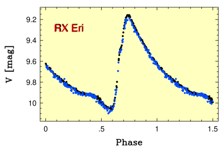
Figure 4: Comparison of the ASAS light curve of RX~Eri (light dots) with that entering in the compilation of JK96 (black dots). The folding period of $0.58724599$ d was derived from the combined dataset spanning 18.7 y. No adjustment of the magnitudes was made.

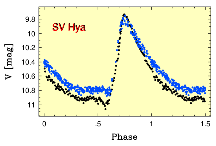
Figure 5: As in Fig. 4, but for SV~Hya. Folding period and total time span are 0.47854709 d and 33.3 y, respectively.

Table 3: Comparison of the light curve parameters

Param.	$\Delta_{1}$	Outliers	$\Delta_{2}$
$P$	$(-3.0\pm 25.1)\times 10^{-6}$	SV Hya, IU Car, RX Cet, TV Leo, RY Psc, AT Vir	$(1.1\pm 3.9)\times 10^{-6}$
$A_{0}$	$-0.016\pm 0.044$	AV Ser, V445 Oph, SV Hya, RY Psc, FY Hya	$\phantom{-}0.001\pm 0.015$
$A_{1}$	$-0.009\pm 0.021$	RY Psc, RX Cet, SV Hya, FY Hya, AV Ser, IU Car,	$-0.003\pm 0.005$
		V445 Oph, RZ Cet, BB Pup
$A_{2}$	$-0.006\pm 0.014$	RX Cet, SV Hya, IU Car, AV Ser	$-0.001\pm 0.007$
$A_{3}$	$-0.003\pm 0.012$	RX Cet	$-0.001\pm 0.008$
$A_{4}$	$-0.002\pm 0.012$	RX Cet, RY Psc, IU Car	$-0.001\pm 0.005$
$\varphi_{21}$	$\phantom{-}0.010\pm 0.065$	RZ Cet, RX Cet	$\phantom{-}0.011\pm 0.055$
$\varphi_{31}$	$\phantom{-}0.020\pm 0.114$	RX Cet, IU Car	$\phantom{-}0.000\pm 0.088$
$\varphi_{41}$	$\phantom{-}0.050\pm 0.132$	RX Cet, TV Lib, DH Hya, FY Hya,	$\phantom{-}0.010\pm 0.083$
$\rm[Fe/H]$	$\phantom{-}0.026\pm 0.153$	RX Cet, IU Car	$\phantom{-}0.001\pm 0.119$

Notes: $\Delta_{1}\equiv\langle p({\rm ASAS})-p({\rm JK96})\rangle$, where $p$ denotes the parameter entering in the first column, the $\langle...\rangle$ symbol stands for simple average over the sample of the 31 stars of set #1. The standard deviation of $\Delta_{1}$ is listed after the $\pm$ sign; $\Delta_{2}$ as above, but for the set obtained after $\sim 3\sigma$ outlier selection; outliers are listed in decreasing order of outlier status; $P$ stands for the period, $A_{0}$ for the average magnitude, $A_{i}$ and $\varphi_{i1}$ for the Fourier amplitudes and phases, respectively; units are in [d], [mag], [rad] and in [dex].

In order to assess the overall agreement between the two datasets, we compare the period, the average brightness, the Fourier parameters (up to order 4) and [Fe/H] for set #1. Table 3 shows the average differences and the standard deviations before and after outlier selection. We employed a $\sim 3\sigma$ criterion for outlier selection (here $\sigma$ stands for the standard deviation of the differences between the corresponding parameter values derived from the ASAS and JK96 sets).

We see that the ASAS amplitudes are (on average) slightly smaller than those of JK96. An opposite trend can be observed for the phases. Although the effect is present in all amplitudes and phases, it is near to the $1\sigma$ error limits of these deviations, as can be seen from the standard deviations and the sample size. The standard deviations of the differences ($p({\rm ASAS})-p({\rm JK96})$, where $p$ denotes one of the parameters tested) are fairly small. In terms of the total ranges of the corresponding parameters, they correspond to $3$–$10$% relative scatters.

Pojmanski (2002) also performed a consistency test of the photometric zero points between the ASAS and Hipparcos databases. He concluded that the difference depended on the position of the object on the CCD frame, and in the best case the standard deviation of the differences was $0.018$ mag in the range of $8$–$12$ mag. Our comparison on the limited sample of set #1 supports this result.

From the point of view of the consistency of the [Fe/H] values, after selecting the two outliers, we have an agreement with a standard deviation of $0.119$ dex between the individual estimates. If we extrapolate this standard deviation as a general error of the currently available photometry and we take into consideration that the total standard deviation in the JK96 calibration was only $0.134$ dex, we end up with an unrealisticly small error of $0.062$ dex for the spectroscopic data (assuming a quadratic relation for the errors). Although the $0.119$ dex standard deviation can be decreased down to $0.093$ dex by omitting several other, less significant outliers (RY~Psc, TV~Leo, TY~Pav, U~Lep and SX~For), we think that except if we have long-term accurate photometry, in general we may expect an inaccuracy in the derived Fourier parameters that leads to an error near $0.1$ dex in the predicted iron abundance.

It is difficult to pinpoint the leading source of the lack of higher-level of compatibility between the two datasets. In the case of the older photoelectric data, entering in the compilation of JK96, we usually have short tracks of data sometimes spanning several years. The tracks are, in general, from different sources. Construction of smooth folded light curves from these segments is often ambiguous because of the non-uniqueness of the combination of the data separated by long gaps. The advantage of the ASAS data over these older observations is that they are compact, and that the number of data points per star is relatively large. The disadvantage is the relatively high noise level and the lack of a more accurately defined magnitude system. This latter point was partially tested by checking the interrelations among the Fourier parameters (see JK96 and Kovács & Kanbur 1998). We found a very good overall agreement with the earlier derived relations, which is an indication that the ASAS light curves for RR Lyrae stars must be fairly close to the standard $V$ system.

In discussing the individual outliers listed in Table 3, four stars, RX~Cet, RZ~Cet, SV~Hya and RY~Psc turned out to be Blazhko stars (see Table 1). These variables often appear among the outliers in Table 3. In principle, if they had been observed frequently enough in both datasets, we would expect to recover the same average light curves. Unfortunately, as already mentioned above, the older data are rather sporadic and the ASAS data are somewhat noisy. These result in different Fourier decompositions in the two datasets. Variable FY~Hya is reasonably noisy in both datasets. For V445~Oph we suspect that the high reddening of $E_{\rm B-V}=0.19$ (see L94) might be instrumental in the observed differences for $A_{0}$ and $A_{1}$. Variable AV~Ser is reasonably noisy in the ASAS set with a relatively modest number of data points. The extremely short periodic star TV~Lib appears as an outlier only in $\varphi_{41}$. We do not know the cause of this, but this special object should be further analyzed, because if it is indeed an RRab star, it is very unique (we do not know any other variable classified as RRab-type with such a short period).

The period analysis of the ASAS data on IU~Car, TV~Leo and AT~Vir yielded significantly different periods from the ones used by JK96 (the same is true for three Blazhko stars, but they have already been discussed). Among these period changing stars only IU~Car shows different light curves in the two datasets. A closer inspection of the JK96 data shows that only the data between HJD 2441807 and 2441695 are discrepant, the rest fit the ASAS data. It can also be seen that a shift of $\sim 0.16$ d in the above interval cures the problem. Because of the large gaps in the sampling of IU~Car in the JK96 set, a separate frequency analysis of the light curve of this star in this dataset leads to the selection of an alias period. This solution no longer works when one tries to combine the data with the ASAS set. We note that IU~Car was an ‘unexplained’ outlier in the [Fe/H] fit of JK96. With the correct period its outlier status disappears.

Variables DH~Hya and BB~Pup are marginal outliers. Their status can be changed by a slight modification of the Fourier fitting algorithm, i.e., by using the polynomial fitting method mentioned in JK96.

3 Predicted versus observed abundances

Following the same methodology as in the previous section, here we make a comparison between the spectroscopic and the Fourier metallicities. We discuss the outlying objects, where the outlier status is defined by the arbitrary limit of $0.4$ dex between the difference of the spectroscopic and Fourier metallicities. We note that this limit corresponds to $\sim 3\sigma$ deviation according to the fit of JK96.

3.1 Set #1

In Sect. 2 we compared the Fourier parameters and the predicted [Fe/H] of this set with those of JK96. Here we make a comparison only with the spectroscopic [Fe/H]. In Fig. 6 we show the correlation between the Fourier and spectroscopic [Fe/H]. With the criterion mentioned above, we found a single outlier. For compatibility with the discussion in the next subsection, we summarize the relevant properties of this star in Table 4. The NL classification of the light curves is somewhat subjective but reasonable support was lent by the few tests we made on the formal error of $\varphi_{31}$. The spectroscopic abundance was declared inaccurate (IS) whenever the number of measurements was lower than three or the values measured had standard deviation greater than 0.20. We note that in the database of L94 the number of measurements for the individual objects rarely exceeds five.

Considering the individual objects, we note that the light curve of TY~Pav is fairly noisy and the spectroscopic abundance is based only on two measurements. In the sequence of the degree of discrepancy, the next star is RX~Cet, with $\Delta{\rm[Fe/H]}=-0.34$ dex. This variable shows a strong Blazhko effect and the number of data points seems to be insufficient to obtain a reliable mean light curve that might yield a better fit to the observed abundance (see Alcock et al. 2003 for the similarity of the average light curves of the BL stars to those of the mono-periodic ones). IU~Car is no longer an outlier. With the ASAS data, its predicted abundance differs slightly less than 0.3 dex from the spectroscopic one. For the full sample of 31 stars $\sigma(\Delta{\rm[Fe/H]})=0.16$ dex, whereas with the omission of the single outlier we get $0.13$ dex, i.e., the same level of agreement as that of JK96.

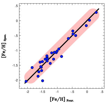
Figure 6: Spectroscopic versus Fourier [Fe/H] computed on 31 stars of the ASAS database (set #1, see Table 1). Shaded area shows the $\pm 0.3$ dex boundaries around the ${\rm[Fe/H]}_{\rm Spec.}={\rm[Fe/H]}_{\rm Four.}$ line.

Table 4: Outliers in [Fe/H] from set #1

Variable	$\Delta$[Fe/H]	Rem
TY Pav	$-0.51$	NL, IS

Notes: $\Delta$[Fe/H]=[Fe/H]${}_{\rm Spec}-$[Fe/H]_Four; BL : Blazhko variable; NL : Noisy light curve; IS : Inaccurate [Fe/H]_Spec; See text for more comments

3.2 Set #2

This set is completely different from the calibration set used by JK96. Therefore, the test presented here constitutes the type of test one is supposed to perform when checking the predictive power of the Fourier method.

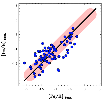
Figure 7: Spectroscopic versus Fourier [Fe/H] computed on 79 stars of the ASAS database (set #2, see Table 2). Notation is the same as in Fig. 6

In a similar presentation as above, Fig. 7 shows the correlation, and Table 5 lists the outliers. We see that there are more outliers than in the case of set #1. This increase is attributed to the lower brightness of the variables in set #2. Because they are fainter, they are less accurately measured both photometrically and spectroscopically. At $V\approx 13$ mag, we are near the faint magnitude limit of the ASAS survey.

Table 5: Outliers in [Fe/H] from set #2

Variable	$\Delta$[Fe/H]	Rem
CK Aps	$0.47$	NL, BL, IS
DD Aps	$0.64$	NL
EL Aps	$-0.56$	IS
ER Aps	$-0.55$	NL, IS
UU Cet	$-0.84$	IS
SX Dor	$-0.79$	NL
SS For	$0.44$	BL, IS
SZ Hya	$0.60$	BL
DG Hya	$0.55$	$-$
FX Hya	$-0.49$	IS
IV Hya	$0.52$	NL, IS
V1023 Oph	$0.41$	NL
TZ Phe	$-0.45$	NL
V765 Sco	$-0.49$	IS
AS Vir	$-0.58$	NL

Notes: Notation is the same as in Table 4.

We see that except for DG~Hya, all outliers can be explained either by high noise in the light curve, the presence of the Blazhko effect or by possible large errors in the abundance. Extreme examples for cases when the noisy light curves are the most probable causes of the discrepancies are DD~Aps and SX~Dor. There are several cases when the spectroscopy can most probably be blamed for the discrepancy. For example, the [Fe/H] values employed in this comparison are based on single measurements for ER~Aps. (Two other stars, LU~Aps and AC~Eri, with lower degree of discrepancy, also have this problem).

The star DG~Hya stands alone with its significant outlier status, not obviously related to its light curve or measured abundance. Indeed, from the Fourier fit and by the application of the error formula of JK96, we get $\sigma({\rm[Fe/H]}_{\rm Four})=0.10$. From the standard deviation and the number of measurements given by L94, we get $\sigma(\langle{\rm[Fe/H]}_{\rm Spec}\rangle)=0.07$. Assuming that these errors are independent, they yield a combined $1\sigma$ error of $0.12$ dex. This makes the observed discrepancy significant above the $4\sigma$ level. We note that for DG~Hya one may end up with a less discrepant Fourier abundance by using the polynomial fitting method mentioned Sect. 2.

In the above outlier selection we relied on objects that correlate tightly and did not make a pre-selection based on the error estimate used above. As already mentioned, the reason for taking this approach is that objects with large errors may accidentally follow the correlation, thereby helping in the selection of the outliers. There are several stars (e.g., UY~Aps, T~Men, RX~Men, etc.) that do not enter in the list of outliers, although it is obvious that they have large errors in their Fourier parameters.

The statistical error formula of JK96 quantifies the ambiguity due to light curve problems and can be used to pre-select candidates that are supposed to yield more accurate Fourier abundances. When applied to the present sample, we may end up with very limited samples by setting the error cutoff at values more preferable for accurate predictions. For example, with $\sigma({\rm[Fe/H]}_{\rm Four})$ cutoffs of $0.3$, $0.2$, $0.15$ and $0.1$, the sample size decreases to $67$, $57$, $48$ and $25$, respectively. Unfortunately, the spectroscopic abundances also have errors, therefore, we need to make further cuts in these already-limited samples if we want to consider all errors consistently. Without this latter cut, even the smallest sample of 25 stars in the above selection yields a large scatter of $0.22$ dex, indicating the presence of spectroscopic errors.

With all $79$ stars left in the sample, we have $\sigma(\Delta{\rm[Fe/H]})=0.31$ dex. By leaving out the 15 outliers as defined at the beginning of this section and listed in Table 5, we get $0.20$ dex. This is in reasonable agreement with the expected scatter based on the calibration set of JK96 if we admit that the data of this separate sample are in general of lower quality than those of the calibrating set and that we left obviously bad quality light curves in the sample.

Further trimming of the sample by applying cuts of $0.3$ and $0.2$ dex leads to sample sizes and dispersions of $55$, $39$ and $0.17$, $0.12$, respectively. We can also repeat this selection procedure on the database obtained by the application of the polynomial Fourier fitting method of JK96. We end up with similar result, yielding, e.g., a dispersion of $0.16$ dex for the remaining $52$ stars at the cutoff value of $0.3$ dex.

3.3 The combination of sets #2 and JK96

To obtain a more comprehensive view of the fit to all available data that are free of outliers, we show the correlation for 145 variables in Fig. 8. This set contains the 64 stars remaining from the ASAS set #2 and the 81 stars remaining from the basic set of JK96, after leaving out the three outliers IU~Car, TZ~Aur and V341~Aql. The standard deviation of the 145 stars is $0.17$ dex, not far from that of the calibrating set of JK96.

In discussing the outliers, we recall that IU~Car has already been dealt with in Sect. 2.1. The outlier status of IU~Car disappeared by the use of ASAS data and the strongly discrepant abundance ($\Delta{\rm[Fe/H]}=0.61$) in the JK96 set is accounted for by a mysterious time shift in one of the data segments of that set. The variable TZ~Aur has a highly non-uniformly sampled light curve, with only 8(!) data points on the descending branch. Actually, with a straightforward Fourier method it cannot be fitted and one has to use a more sophisticated method, such as polynomial fitting preceding the Fourier decomposition, as mentioned in Sect. 2. Furthermore, there is only one measurement for [Fe/H] in L94 and the five measurements of S94 are rather noisy, yielding an error ($1\sigma$ range) of $0.11$ dex in the published mean metallicity. V341~Aql has $\Delta{\rm[Fe/H]}=0.41$ dex, with an apparently well-established abundance, with two and ten measurements in the compilations of L94 and S94, respectively. The light curve has low scatter, spanning nearly four years with more than 500 data points. It seems to us that the outlier status of V341~Aql cannot be explained by observational noise.

In summary, in the full sample of 163 stars consisting of the ASAS database and the compilation of JK96, we found only two stars, DG~Hya and V341~Aql, whose observed abundances cannot be predicted within 0.4 dex with the Fourier formula of JK96 and whose discrepant status is not easily explained by observational errors only.

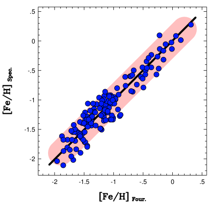
Figure 8: Spectroscopic versus Fourier [Fe/H] computed on the outlier-free sample of 145 stars from the ASAS database and from the compilation of JK96. See text for details on the outlier selection. Notation is the same as in Fig. 6

4 Conclusions

With the accumulating photometric data on RR Lyrae stars, it becomes increasingly interesting to utilize methods that are capable of deriving physical parameters based on the morphology of the light curves. Of course, all methods should be thoroughly tested before they are applied on a target dataset. In this paper we performed such a test on the metallicity determination of the fundamental mode RR Lyrae stars.

The calibration is based on a sample of 81 Galactic field RRab stars by Jurcsik & Kovács (1996). The testing set comes from the ASAS database (Pojmanski 2002, 2003; Pojmanski & Maciejewski 2004). Only those variables were selected from the database that had corresponding low-dispersion spectroscopic metallicities either in Layden (1994) or in Suntzeff et al. (1994). The final ASAS sample contains 110 stars, 31 of them overlap with the compilation of Jurcsik & Kovács (1996). We did not apply any quality control in the selection procedure. We use all light curves irrespective of whether they have mono-periodic light curves of low- or high-noise or show the Blazhko effect. This approach is opposite to the one we followed in the construction of the calibration set. The purpose of the present approach is to make allowance for less favorable cases, when the high noise level or the short time span of the observations do not make a more critical selection possible.

The result of the comparison shows that almost all objects deviating by more than $0.4$ dex from the spectroscopic values exhibit some (well-demonstrated) problems either in the light curve or in the spectroscopy. We have only two objects (V341~Aql and DG~Hya) whose discrepant positions cannot be explained by these simple causes. The outlier-free sample of 64 stars distinct from the calibrating sample reproduces the spectroscopic abundances with a standard deviation of $0.20$ dex. When this ASAS sample is combined with the original calibrating sample of 81 stars (also free of outliers), the standard deviation becomes $0.17$ dex, not far from the fitting accuracy of the calibrating set.

Although the above result is satisfactory in terms of the dispersion between the computed and measured metallicities, it may be far from the accuracy we could reach with better metallicities and light curves. The quality of the light curves can be improved by employing larger aperture telescopes. With the current sophisticated data reduction methods (e.g., image subtraction, see Alard 2000) an accuracy of $0.01$–$0.02$ mag per data point could be routinely reached with a $\sim 20$ cm telescope for stars of $12$–$13$ mag. Long-term monitoring (from months to years) is necessary to obtain sufficient coverage for Blazhko variables. Based on the result of Alcock et al. (2003), it is possible that the average light curves of the Blazhko stars can be employed equally well in the empirical formulae calibrated on strictly periodic stars. This conjecture is partially supported by the present study, because several Blazhko stars did stay in the set after outlier selections. It is highly probable that the situation can be further improved by gathering more data points and covering the Blazhko cycle more fully.

A real improvement may come from a renewed effort to gather more accurate spectroscopic data. Ambiguities due to pulsation phase dependence should be minimized by taking more observations per object. The fact that globular cluster giants are often measured with an accuracy higher than $0.1$ dex implies that high-dispersion data could reach similar accuracy once the phase dependence is appropriately taken care of. The goal of good phase coverage can, of course, be reached more easily by taking low-dispersion spectra and using a spectral index method. However, these spectral index methods should be calibrated directly by the updated accurate high-dispersion abundances mentioned above.

To target individual variables with the Fourier method and aiming at accurate abundance estimates on specific objects, one has to be sure that the formula is applicable to any RRab star. Currently, with the two unexplained outliers, we have a chance of $\sim 1$% of hitting such an object in a randomly selected target list. Although this is a relatively small chance, for a more consistent assessment of the outlier status of the individual objects, we would need better error estimates of the spectroscopic abundances. With the few data points per variable and the lack of more precise knowledge of the phase dependence of the [Fe/H] estimates, the required reliable error estimation is not possible.

In principle, if the relation between [Fe/H] and the Fourier parameters indeed holds for the overwhelming majority of RRab stars, because of the general statistical property of a regression to noisy data, we expect more accurate [Fe/H] estimates from the Fourier method than from direct spectroscopic measurements. Therefore, it will become more interesting to address the physical origin of this relation. Unfortunately, the cause of this relation is unknown at the moment. On the empirical side, in a recent paper Sandage (2004) attempts to derive the $P$–$\varphi_{31}$–[Fe/H] relation on the basis of other empirical relations, exploring the correlations among the various light curve parameters, without giving any explanation for the existence of the formula for [Fe/H]_Four. On the theoretical side, except for a note by Bono, Incerpi & Marconi (1996) and for some partial results of Feuchtinger & Dorfi (1997) and Dorfi & Feuchtinger (1999) there are no works targeting the background of this relation. Although in the latter papers we find that the models show the predicted trends (i.e., increase of $\varphi_{31}$ with the increase of $P$, shifting the [Fe/H]=const ridge lines on the $P\rightarrow\varphi_{31}$ plots), no quantitative comparison is possible because of the limited scope of the theoretical surveys. This situation further emphasizes the need for accurate spectroscopic abundances that are capable of helping in the derivation of a tighter calibration formula, whereby the theoretical models can be confronted with more stringent empirical constraints.

Until then, with the current fitting accuracy of $0.17$ dex of the Fourier formula, we conservatively estimate the overall prediction accuracy, i.e., the standard deviation of the predicted [Fe/H], to be $0.12$ dex (by sharing the total error budget equally between the Fourier parameters and the spectroscopic abundances). This accuracy makes the Fourier method a useful tool for the estimation of the abundances of various populations of RR Lyrae stars but limits its applicability in individual cases, where higher accuracy might be demanded.

- (1) Alard, C., 2000, A&AS, 144, 363
- (2) Alcock, C. et al., The macho collab., 2003, ApJ, 598, 597
- (3) Borissova, J., Minniti, D., Rejkuba, M., Alves, D., Cook, K. H., Freeman, K. C., 2004, A&A, 423, 97
- (4) Bono, G., Incerpi, R. & Marconi, M., 1996, ApJ, 467, L97
- (5) Butler, D., Dickens, R. J. & Epps, E., 1978, AJ, 225, 148
- (6) Butler D., Manduca A., Deming D. & Bell R. A., 1982, AJ 87, 640
- (7) Clementini, G., Merighi, R., Gratton, R., Carretta, E., 1994, MNRAS, 267, 43
- (8) Clementini, G., Carretta, E., Gratton, R., Merighi, R., Mould, J. R., McCarthy, J. K., 1995, AJ, 110, 2319
- (9) Dorfi, E. A. & Feuchtinger, M. U., 1999, A&A, 348, 815
- (10) Fernley, J. & Barnes, 1996, A&A, 312, 957
- (11) Feuchtinger, M. U. & Dorfi, E. A., 1997, A&A, 322, 817
- (12) Gratton, R. G.; Bragaglia, A., Clementini, G., Carretta, E., Di Fabrizio, L., Maio, M., Taribello, E., 2004, A&A, 421, 937
- (13) Jurcsik, J., 1995, Acta Astr., 45, 653
- (14) Jurcsik, J., 2003, A&A, 403, 587
- (15) Jurcsik, J. & Kovács, G. 1996, A&A, 312, 111 (JK96)
- (16) Kolláth, Z., 1990, Occ. Techn. Notes Konkoly Obs., 1, http://www.konkoly.hu/staff/kollath/mufran.html
- (17) Kovács, G. Bakos, G. & Noyes, R. W., 2005, MNRAS, 356, 557
- (18) Kovács, G. & Kanbur, S. M. 1998, MNRAS, 295, 834
- (19) Lambert, D. L., Heath, J. E., Lemke, M. & Drake, J., 1996, ApJS, 103, 183
- (20) Layden A. C., 1994, AJ, 108, 1016 (L94)
- (21) Layden A. C., 1997, PASP, 109, 524
- (22) Moskalik, P. & Poretti, E. 2003, A&A, 398, 213
- (23) Pojmanski, G. 2002, Acta Astr., 52, 397 (astro-ph: 0210283)
- (24) Pojmanski, G. 2003, Acta Astr., 53, 341.(astro-ph: 0401125)
- (25) Pojmanski, G. & Maciejewski, G., 2004, Acta Astr., 54, 153. (astro-ph: 0406256)
- (26) Preston, G. W., 1959, ApJ, 130, 507
- (27) Rey, S-C., Lee, Y-W., Joo, J-M., Walker, A. & Baird, S., 2000, AJ, 119, 1824
- (28) Sandage, A., 2004, AJ, 128, 858
- (29) Sandstrom, K., Pilachowski, C. A. & Saha, A., 2001, AJ, 122, 3212
- (30) Schmidt, E. G. & Seth, A., 1996, AJ, 112, 2769
- (31) Schwarzenberg-Czerny, A. & Kaluzny, J., 1998, MNRAS, 300, 251
- (32) Szeidl B., 1988, in Multimode Stellar Pulsations, Eds.: G. Kovács, L. Szabados, B. Szeidl, p. 45
- (33) Suntzeff, N. B., Kraft, R. P. & Kinman T. D., 1994, ApJS, 93, 271 (S94)
- (34) Wozniak, P. R., Vestrand, W. T., Akerlof, C. W. et al., 2004, AJ, 127, 2436