The 2dF-SDSS LRG and QSO Survey: The $z<2.1$ Quasar Luminosity Function from 5645 Quasars to $g=21.85$

Abstract

We have used the 2-degree Field (2dF) instrument on the Anglo-Australian Telescope to obtain redshifts of a sample of $z<3$, $18.0<g<21.85$ quasars selected from Sloan Digital Sky Survey (SDSS) imaging. These data are part of a larger joint programme between the SDSS and 2dF communities to obtain spectra of faint quasars and luminous red galaxies, namely the 2dF-SDSS LRG and QSO Survey (2SLAQ). We describe the quasar selection algorithm and present the resulting number counts and luminosity function of 5645 quasars in 105.7 deg². The bright end number counts and luminosity function agree well with determinations from the 2dF QSO Redshift Survey (2QZ) data to $g\sim 20.2$. However, at the faint end the 2SLAQ number counts and luminosity function are steeper (i.e. require more faint quasars) than the final 2QZ results from Croom et al. (2004), but are consistent with the preliminary 2QZ results from Boyle et al. (2000). Using the functional form adopted for the 2QZ analysis (a double-power law with pure luminosity evolution characterized by a 2nd order polynomial in redshift), we find a faint end slope of $\beta=-1.78\pm 0.03$ if we allow all of the parameters to vary and $\beta=-1.45\pm 0.03$ if we allow only the faint end slope and normalization to vary (holding all other parameters equal to the final 2QZ values). Over the magnitude range covered by the 2SLAQ survey, our maximum likelihood fit to the data yields 32 per cent more quasars than the final 2QZ parameterization, but is not inconsistent with other $g>21$ deep surveys for quasars. The 2SLAQ data exhibit no well defined “break” in the number counts or luminosity function, but do clearly flatten with increasing magnitude. Finally, we find that the shape of the quasar luminosity function derived from 2SLAQ is in good agreement with that derived from type I quasars found in hard X-ray surveys.

1 Introduction

We have merged the high-quality digital imaging of the Sloan Digital Sky Survey (SDSS; York et al. 2000) and the powerful spectroscopic capabilities of the 2-degree Field (2dF) instrument (Lewis et al. 2002) to conduct a deep wide-field spectroscopic survey for quasars and luminous red galaxies (LRGs), i.e. the 2dF-SDSS LRG and QSO Survey (hereafter referred to as “2SLAQ”). The combination of these facilities allows us to probe substantially deeper than either the SDSS or 2dF surveys can individually. This paper describes the first results of the quasar aspect of the survey; see Cannon et al. (2003), Padmanabhan et al. (2004) and Cannon et al. (2005) for a discussion of the LRG component of the survey.

The 2dF QSO Redshift survey (2QZ; Boyle et al. 2000; Croom et al. 2004) was restricted to $b_{J}<20.85$. We use the SDSS imaging data as the input for a new survey, allowing us to probe to $g=21.85$ with typical photometric errors at the flux limit of only 7 per cent – considerably fainter than either the $i=19.1$ flux limit of the SDSS Quasar Survey (Richards et al. 2002; Schneider et al. 2003) or the $b_{J}=20.85$ flux limits of 2QZ. By allocating 200 fibres per 2dF plate to this new quasar survey (with an additional 200 fibres going to LRGs), and extending the exposure time to 4 hours (compared to $\sim 1$ hour for SDSS and 2QZ), we hope to obtain spectra of 10,000 quasars to $g=21.85$ in the next few years. This paper reports on the first three semesters of data (with 5645 quasars) and presents the $z<2.1$ quasar luminosity function (QLF) to fainter luminosities at each redshift than either the SDSS or 2QZ surveys alone.

The first determination of the luminosity function of quasars was by Schmidt (1968). Subsequent pioneering work was carried out by many groups including Schmidt & Green (1983), Koo & Kron (1988), Hewett, Foltz & Chaffee (1993) and especially Boyle and collaborators (e.g. Boyle, Shanks & Peterson 1988), with extensions to high-$z$ ($z>3$) being provided by Warren, Hewett & Osmer (1994), Schmidt, Schneider & Gunn (1995), Kennefick, Djorgovski & de Carvalho (1995) and Fan et al. (2001b). The largest samples analysed to date come from the 2dF QSO Redshift Survey (Boyle et al. 2000; Croom et al. 2004) with 23,338 quasars.

With the exception of variability-selected samples (e.g. Hawkins & Veron 1995), early QLF determinations were generally characterized by a strong, distinct “break” whose redshift evolution has been the subject of much discussion. However, more recent determinations (e.g. COMBO-17; Wolf et al. 2003), while still exhibiting distinct curvature in a log-log plot, show less of a break at a specific luminosity.

Recently, optical surveys have been supplemented by X-ray surveys (both soft and hard) that, when correcting for selection differences, can largely reproduce the optical type I QLF (e.g. Ueda et al. 2003; Barger et al. 2005). These X-ray QLFs have also been shown to exhibit a break, but generally at luminosities much fainter than found by optical surveys; this result suggests incompleteness at the faint end of optical surveys.

As we shall see, our data are in good agreement with recent results for faint quasars from both the optical (e.g. Wolf et al. 2003) and X-ray (e.g. Barger et al. 2005). We probe nearly 1 magnitude deeper than 2QZ, and find that the faint end slope of the QLF is steeper than that of the most recent 2QZ determination and lacks a strong characteristic break feature, but is still better characterized by a double-power law than a single power-law.

Section 2 presents a description of the imaging data and the sample selection. In Section 3 we describe the observations and data reduction. Section 4 presents the completeness corrections leading to the QLF presented in in § 5. Finally, § 6 presents a discussion of the ramifications of our work and summarizes our results. Throughout this paper we use a cosmology with $H_{o}=h_{70}70$ km s^-1 Mpc^-1, $\Omega_{m}=0.3$, $\Omega_{\Lambda}=0.7$ (e.g. Spergel et al. 2003).

2 The imaging data and sample selection

2.1 The SDSS imaging data

The photometric measurements used as the basis for our catalogue are drawn from SDSS imaging data (DR1 reductions; Stoughton et al. 2002; Abazajian et al. 2003), which will eventually cover roughly 10,000 deg² of sky in five photometric passbands ($ugriz$) using a large-format charge-coupled device (CCD) camera (Gunn et al. 1998). The photometric system and its characterization are discussed by Fukugita et al. (1996), Hogg et al. (2001), Smith et al. (2002) and Stoughton et al. (2002); the spectroscopic tiling algorithm is described by Blanton et al. (2003). Except where otherwise stated, all SDSS magnitudes discussed herein are “asinh” point-spread-function (PSF) magnitudes (Lupton, Gunn & Szalay 1999) on an AB magnitude system (Oke & Gunn 1983) that have been dereddened for Galactic extinction according to the model of Schlegel, Finkbeiner & Davis (1998). The astrometric accuracy of the SDSS imaging data is better than 100 mas per coordinate rms (Pier et al. 2003). The SDSS Quasar Survey (Richards et al. 2002; Schneider et al. 2003, 2005) extends to $i=19.1$ for $z<3$ and $i=20.2$ for $z>3$, whereas our work herein explores the $z<3$ regime to $g=21.85$ ($i\sim 21.63$).

2.2 Preliminary sample restrictions

Our quasar candidate sample was drawn from 10 SDSS imaging runs (see § 2.4) after having first been vetted of objects that have cosmetic defects (e.g. bad columns) that might cause the photometry to be inaccurate. Specifically, we rejected any objects that met the “fatal” or “non-fatal” error definitions as described by Richards et al. (2002).

We next imposed limits on the $i$-band PSF magnitude and its estimated $1\sigma$ error of $i<22.0$ and $\sigma_{i}<0.2$. Further magnitude cuts are done in the $g$-band (to facilitate comparisons with previous 2QZ results in $b_{J}$); the $i$-band cuts are primarily to reduce the number of objects that we have to examine initially. We also placed restrictions on the errors in each of the other four bands, specifically, $\sigma_{u}<0.4$, $\sigma_{g}<0.13$, $\sigma_{r}<0.13$ and $\sigma_{z}<0.6$. These restrictions are designed to ensure that the errors on the magnitudes are reasonably small (and thus that the resulting colours are accurate), but also are sufficiently relaxed that, when coupled with the magnitude cut in $i$ and $g$, objects with quasar-like continua are not rejected. This tolerance is necessary since, as we go fainter, restrictions on magnitude errors are effectively cuts in magnitude and any two such restrictions are effectively colour cuts. Note that this selection of error constraints effectively limits the redshift to less than 3, as the Ly$\alpha$ forest suppresses the $u$ flux at higher redshifts.

2.3 Colour cuts

Based on spectroscopic identifications from SDSS and 2QZ of this initial set of objects, we implement additional colour cuts that are designed to efficiently select faint quasars while maintaining a high degree of completeness to known UV-excess broad-line quasars. An analysis of the completeness of the selection algorithm is given as a function of redshift and magnitude in § 4.2.

We first impose colour restrictions that are designed to reject hot white dwarfs. These cuts are made regardless of magnitude. Specifically, we rejected objects that satisfy the condition: $A\&\&((B\&\&C\&\&D)||E)$, where the letters refer to the cuts:

$$\begin{array}[]{rrcccl}{\rm A})&-1.0&<&u-g&<&0.8\\ {\rm B})&-0.8&<&g-r&<&0.0\\ {\rm C})&-0.6&<&r-i&<&-0.1\\ {\rm D})&-1.0&<&i-z&<&-0.1\\ {\rm E})&-1.5&<&g-i&<&-0.3.\end{array}$$ (6)

This is similar to the white dwarf cut applied by Richards et al. (2002, Equation 2) except for the added cut with respect to the $g-i$ colour.

As the targets become fainter and the magnitude errors increase, we find that maximizing our completeness and efficiency is best served by separate handling of bright and faint objects. The bright sample is restricted to $18.0<g<21.15$ and is designed to allow for overlap with previous SDSS and 2dF spectroscopic observations. The faint sample has $21.15\leq g<21.85$ and probes roughly one magnitude deeper than 2QZ. These cuts are made in $g$ rather than $i$ (as the SDSS quasar survey does) since we are concentrating on UV-excess quasars and would like to facilitate comparison with the results from the $b_{J}$-based 2QZ. The combination of the $g<21.85$ and $i<22.0$ cut will exclude objects bluer than $\alpha_{\nu}=+0.3\;(f_{\nu}\propto\nu^{\alpha})$; however, objects this blue are exceedingly rare ($>3\sigma$ deviations).

Further cuts are made as a function of colour and morphology in each of the bright/faint samples. In general, we would prefer not to make a cut on morphology since we do not want to exclude low-$z$ quasars and because our selection extends beyond the magnitude limits at which the SDSS’s star/galaxy separation breaks down. However, Scranton et al. (2002) have developed a Bayesian star-galaxy classifier that is robust to $r\sim 22$. As a result, in addition to straight colour-cuts, we also apply some colour restrictions on objects with high $r$-band galaxy probability (referred to below as “galprob”) according to Scranton et al. (2002) in an attempt to remove contamination from narrow emission line galaxies (NELGs; i.e. blue star-forming galaxies) from our target list.

Bright sample objects are those with $18.0<g<21.15$ and that meet the following conditions

$$\begin{array}[]{rcclcccll}{\rm A})&u-g&<&0.8&\&\&&g-r&<&0.6&\&\&\\ &r-i&<&0.6&&&&&\\ {\rm B})&u-g&>&0.6&\&\&&g-i&>&0.2&\\ {\rm C})&u-g&>&0.45&\&\&&g-i&>&0.35&\\ {\rm D})&{\rm galprob}&>&0.99&\&\&&u-g&>&0.2&\&\&\\ &g-r&>&0.25&\&\&&r-i&<&0.3&\\ {\rm E})&{\rm galprob}&>&0.99&\&\&&u-g&>&0.45.&\end{array}$$ (14)

in the combination $A\&\&!B\&\&!C\&\&!D\&\&!E$, where cut A selects UVX objects, cuts B and C eliminate faint F-stars whose metallicity and errors push them blueward into the quasar regime, and cuts D and E remove NELGs that appear extended in the $r$ band. Among the bright sample objects, those with $g>20.5$ were given priority in terms of fibre assignment.

Faint sample objects are those with $21.15\leq g<21.85$ and that meet the following conditions

$$\begin{array}[]{rcclcccll}{\rm A})&u-g&<&0.8&\&\&&g-r&<&0.5&\&\&\\ &r-i&<&0.6&&&&&\\ {\rm B})&u-g&>&0.5&\&\&&g-i&>&0.15\\ {\rm C})&u-g&>&0.4&\&\&&g-i&>&0.3\\ {\rm D})&u-g&>&0.2&\&\&&g-i&>&0.45\\ {\rm E})&{\rm galprob}&>&0.99&\&\&&g-r&>&0.3.\end{array}$$ (21)

in the combination $A\&\&!B\&\&!C\&\&!D\&\&!E$, where cut A selects UVX objects, cuts B, C and D eliminate faint F-stars whose metallicity and errors push them blueward into the quasar regime, and cut E removes NELGs. These faint cuts are more restrictive than the bright cuts to avoid significant contamination from main sequence stars that will enter the sample as a result of larger errors at fainter magnitudes.

Figure 1 shows the $u-g$ vs. $g-i$ colour distribution of objects satisfying these criteria for which we obtained new spectra. Objects confirmed to be quasars are shown in black, while those that are not quasars (mostly stars and NELGs) are shown in red. The locus of $z<3$ quasars from SDSS-DR1 (Schneider et al. 2003) is given by grey contours and points. Solid blue, dashed blue and dotted cyan lines show the faint sample colour cuts, the bright sample colour cuts and the white dwarf cut, respectively.

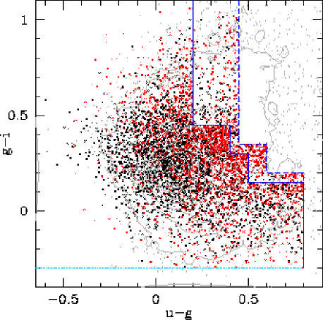
Figure 1: Colours of spectroscopically identified 2SLAQ targets. Confirmed quasars are shown in black, non-quasars in red. For reference the colour distribution of $z<3$ SDSS-DR1 quasars (Schneider et al. 2003) are shown as faint grey contours/points. The dashed and solid dark blue lines show the $u-g$ and $g-i$ colour cuts for the bright and faint samples, respectively. The dotted cyan line shows the boundary of the $g-i$ cut used to reject white dwarfs.

2.4 Sky location of imaging data

2.4.1 2003A and 2004A

For the first semester both of 2003 and 2004, we used the SDSS imaging data (rerun 20; Stoughton et al. 2002; Abazajian et al. 2003) in the SDSS northern equatorial scan (stripe 10) from runs 752, 756, 1239 and 2141; see York et al. (2000) and Stoughton et al. (2002) for the definition of the relevant SDSS technical terms. Run 756 was used for the northern part of the stripe, while a combination of the other three runs was used for the southern part of the stripe in an attempt to use the best quality data (typically that with the best seeing). The area of sky sampled was further limited to regions where the SDSS image quality was deemed to be good enough to use for targeting faint objects for spectroscopy, specifically seeing $\leq 1\aas@@fstack{\prime\prime}8$ and $r$-band Galactic extinction $\leq 0.2$ (Schlegel et al. 1998). We also excluded any objects from SDSS camera column 6, since 2dF cannot cover the full 2.5 degree wide SDSS stripe and column 6 has the lowest quality data of all the columns as a result of (relatively) poorer image quality at the edge of the camera in these early SDSS data. The final RA ranges were $123\mbox{${}^{\circ}$}<\alpha_{\rm J2000}<144\mbox{${}^{\circ}$}$, $150\mbox{${}^{\circ}$}<\alpha_{\rm J2000}<168\mbox{${}^{\circ}$}$, $185\mbox{${}^{\circ}$}<\alpha_{\rm J2000}<193\mbox{${}^{\circ}$}$, $197\mbox{${}^{\circ}$}<\alpha_{\rm J2000}<214\mbox{${}^{\circ}$}$ and $218\mbox{${}^{\circ}$}<\alpha_{\rm J2000}<230\mbox{${}^{\circ}$}$. Whenever possible, we tried to overlap areas with existing 2QZ spectroscopy to limit the number of objects with $b_{J}<20.85$ that needed spectroscopic confirmation. SDSS spectroscopy limits the need for new $i<19.1$ spectra. The two top panels of Figure 2 illustrate the area covered by our Semester A targets ($-1.259\mbox{${}^{\circ}$}\leq\delta_{\rm J2000}\leq 0.840\mbox{${}^{\circ}$}$).

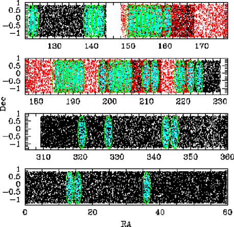
Figure 2: RA and Dec distribution of 2dF targets selected from SDSS imaging data (black) and previous 2dF observations (red). 2SLAQ observations are given by cyan points within 41 plates (green circles). The top two panels are semester A targets; the bottom two panels are semester B targets. Note the distortion of the coordinate system; the spectroscopic plates are actually circular.

2.4.2 2003B

For the second semester, our samples were limited to the following combination of data (run, rerun, strip, $\alpha_{\rm J2000}$ range): (2659, 40, 82N, $309.20\mbox{${}^{\circ}$}<\alpha_{\rm J2000}<320.34\mbox{${}^{\circ}$}$), (2662, 40, 82N, $320.34\mbox{${}^{\circ}$}<\alpha_{\rm J2000}<15.08\mbox{${}^{\circ}$}$), (2738, 40, 82N, $15.08\mbox{${}^{\circ}$}<\alpha_{\rm J2000}<59.70\mbox{${}^{\circ}$}$), (2583, 40, 82S, $309.20\mbox{${}^{\circ}$}<\alpha_{\rm J2000}<341.08\mbox{${}^{\circ}$}$), (3388, 40, 82S, $341.08\mbox{${}^{\circ}$}<\alpha_{\rm J2000}<345.44\mbox{${}^{\circ}$}$), (3325, 41, 82S, $345.44\mbox{${}^{\circ}$}<\alpha_{\rm J2000}<59.70\mbox{${}^{\circ}$}$). These reruns (40 and 41) represent post-DR1 data processing, which includes a newer version of the photometric pipeline and improved photometric calibration. Again, camera column 6 was excluded and these are all equatorial scans. Note that there are no 2QZ observations in this range. The two bottom panels of Figure 2 illustrate the area covered by our Semester B targets.

2.4.3 Sky area

The area of sky covered by our catalogue of targets for 2003/4A was 159.4 deg² with 20228 targets and for 2003B it was 230.2 deg² with 33160 total targets. Thus we have a total area of 389.6 deg² and 53388 targets. Of this area, this paper concentrates on only those regions where we have obtained new spectra (see Figure 2). In semester 2003/4A, 34 plates were observed, covering an area of 80.82 deg² – as determined by the fraction of targets within the plate areas (11075 of 53388). In the second semester, seven plates were observed, covering an area of 24.9 deg² (3407 of 53388 targets within the new plate areas). Note that the plates overlapped in 2003/4A, but not in 2003B. The theoretical area for 2003B given a plate radius of 1.05 deg is $24.3$ square degrees, which compared to the area estimated by fraction of targets (24.9 deg²) suggests that our estimate of the area has a roughly 2.5 per cent error. Thus the area covered by new plate observations is $105.7\pm 2.6$ deg². Within these plate centers there are 14482 targets, of which 9120 have spectroscopic identifications, and among those are 5645 quasars.

3 Spectroscopic observations

3.1 The 2dF facility

The Two Degree Field (2dF; Lewis et al. 2002) facility at the Anglo-Australian Telescope is a fibre fed multi-object spectrograph and robotic fibre positioner. The fibres are $140\mu$m in diameter, which is roughly $2\aas@@fstack{\prime\prime}16$ at the centre of the plate and $1\aas@@fstack{\prime\prime}99$ at the edges. Two independent spectrographs use Tektronix 1024$\times$1024 CCDs with a range of diffraction gratings offering resolutions between 10Å and 2.2Å over the optical wavelength range. During standard operation, 400 fibres are available for simultaneous observation (200 per spectrograph) over a 2 degree diameter field of view. The system is equipped with an atmospheric dispersion compensator which enables 2dF observations to be taken over a wide wavelength range, by ensuring that all wavelengths from the UV to NIR enter the fibres. However, differential spatial atmospheric refraction distorts the field geometry and limits observations of equatorial fields to $\pm 1$ hour on either side of transit.

3.2 2dF field configurations

The 2SLAQ survey regions are centred close to the equator and are 2 degrees wide in declination. To achieve optimal sky coverage while still retaining a largely contiguous area, the 2dF field centres are placed along the central declination of the two strips; $\delta_{\rm J2000}=-00^{\circ}12\arcmin 35\arcsec$ for the North Galactic Pole (NGP) strip and $\delta_{\rm J2000}=-00^{\circ}15\arcmin 00\arcsec$ for the South Galactic Pole strip; see § 2.4. Each field centre is separated by 1.2 degrees, although some early observations of the NGP at the start of 2003 had field spacings of 1 degree.

The target list generated from the process described in § 2 is then merged with a target list of LRGs selected from the same photometric data set (Cannon et al. 2005). The sub-samples within this combined data set are assigned different priorities which determine the likelihood of a fibre being assigned to them in the 2dF configuration process. The priority values given to each sample are listed in Table 1, where 9 is the highest and 1 the lowest priority. All available high priority targets are allocated before moving to the next priority level. For source densities much greater than 400 per 2dF field, the 2dF configuration algorithm will tend to give a non-uniform distribution of fibres allocated to objects (Cannon et al. 2005). Therefore the main samples of each of the LRG and QSO data sets were randomly sampled to a surface density of 200 per 2dF field and these given priority 8 and 6 for the LRGs and QSOs respectively. The remaining sources from these main samples were given lower priority (7 and 5 respectively). Other sub-samples, such as bright QSOs and high-redshift candidates, were given lower priority.

For the QSO sample we used the low resolution 300B grating (as used for the 2QZ), but the LRG observations required the use of the higher resolution 600V grating. Therefore, one of the 2dF spectrographs is configured with a 300B grating (spectrograph 1) while the second (spectrograph 2) is configured with the 600V grating. On each 2dF field plate of 400 fibres, each block of 10 fibres (a retractor block) goes to an alternate spectrograph, so that 200 fibres on each plate are available for the QSOs and 200 for the LRGs. 2dF fibres are limited to a maximum off-radial angle of 14 degrees, therefore there are 20 small triangles surrounding the edge of the 2dF fields that are inaccessible to the QSO spectrograph covering a total area of 0.43 deg². The angular completeness function defined by this complex field pattern is not relevant to the QLF analysis below, but it is critical to accurate measurements of clustering. Of the 200 fibres available for the QSOs, 20 were allocated to positions known to be blank sky to be used for sky subtraction.

Table 1: 2dF configuration priorities.

Sample	Priority
Guide stars	9
LRG (main) random	8
LRG (main) remainder	7
QSOs ($g>20.5$) random	6
QSOs ($g>20.5$) remainder	5
LRG(extras)+hi-z QSOs	4
QSOs ($g<20.5$)	3
previously observed	1

3.3 2dF observations and data processing

Observations started in March 2003. Each 2dF field was observed for a minimum of four hours (more if weather was poor). These four hours were split over two nights to minimize the effects of changing atmospheric refraction. The 300B grating used gives a dispersion of 4.3Å pixel^-1 and an instrumental resolution of 9Å. The spectra cover the range 3700-7900Å. The data were reduced in real time using the standard 2dFdr pipeline (Bailey et al. 2003, MNRAS submitted). The exposure times increased if the conditions meant that a pre-defined completeness limit (80 per cent) was not met. Any source that has a high S/N spectrum and a high-confidence identification after the first night of observation has its fibre assigned to previously unallocated sources for future observations of the field.

The identification of QSOs and measurement of redshifts was done using the AUTOZ code that was developed for the 2QZ (see Croom et al. (2001, § 3.1) and Croom et al. (2004, § 2.3.1) for details). All spectra are then checked by eye to confirm the identifications. Since spectroscopic processing is the same as that used for 2QZ spectra (e.g., quasars must have broad [$>1000\,{\rm km\,s^{-1}}$] emission lines), we treat 2SLAQ selected objects with 2QZ spectra as if they were observed as part of the 2SLAQ programme.

4 Completeness corrections

In this section we explore and quantify the various effects that will bias the quasar number counts and luminosity function. In particular, we address the photometric, coverage, spectroscopic and cosmetic defect incompleteness of our sample. In addition, we investigate the difference between $g$ and $b_{J}$ magnitudes, Eddington bias, morphology bias and the effects of variability.

4.1 Coverage and spectroscopic completeness

We have not obtained spectra of all our quasar candidates in the 105.7 deg² analyzed in this paper. Thus we must compute the “coverage” completeness of our sample, which multiplied by the area yields the effective area of the survey. Since we are combining data from three distinct surveys (SDSS, 2QZ, and 2SLAQ) in order to increase our dynamic range, it is necessary to compute this correction as a function of magnitude. The coverage completeness is computed under the assumption that the fraction of objects that remain unobserved (at a given magnitude) will be quasars at the same rate as those that are observed. This assumption is reasonable given that the objects observed are chosen at random. Figure 3 shows the coverage completeness (solid line) that we compute as a function of magnitude.

Figure 3: Spectroscopic (dashed line) and coverage (solid line) completeness fractions as a function of magnitude in 0.25 mag bins. These corrections were applied (in conjunction with the photometric completeness correction [Fig. 4]) to determine the corrected number counts. The dotted vertical lines show the boundaries of the SDSS ($i=19.1$, $g\sim 19.32$) and 2QZ surveys ($b_{J}\sim g=20.85$). The discontinuity in coverage completeness at $g\sim 20.5$ is caused by a prioritization of targets fainter than this limit; see Table 1.

In addition to the coverage completeness, we must correct for those cases in which our spectroscopy does not yield an unambiguous identification. Assuming that the fraction of unidentified objects will be quasars at the same rate as those among identified objects (as a function of magnitude), we derive a spectroscopic incompleteness as shown by the dashed line in Figure 3. This assumption arguably may tend to overestimate the number of unidentified quasars since the spectroscopic completeness may additionally be a function of redshift (because of emission line effects which generally facilitate quasar identification) and that any completeness determination is surely to be a lower-limit. However, our spectroscopic completeness is generally high (70 per cent at the faint limit, 90 per cent brighter), thus any second-order corrections will have a minimal impact. Furthermore, comparison with supplementary identifications based solely on photometry and photometric redshifts (§ 5) suggests that this assumption is reasonable. In practice we have treated the spectroscopic completeness as if the unidentified objects simply had not been observed, which facilitates the application of these corrections to our model of the luminosity function.

4.2 Photometric completeness

The incompleteness of our sample due to colour cuts is a strong function of both redshift and magnitude since the colours of quasars change significantly with redshift and fainter quasars have larger errors. We quantify this incompleteness by running our selection algorithm on a sample of simulated quasars that were designed to test the SDSS’s quasar target selection algorithm; see Fan (1999) and Richards et al. (2005). The primary independent variable in the simulations is the spectral index distribution, which is given by a Gaussian distribution with $\alpha_{\nu}=-0.5\pm 0.3\;(f_{\nu}\propto\nu^{\alpha_{\nu}})$, which is in good agreement with the composite SDSS quasar spectrum given by Vanden Berk et al. (2001). Blueward of the Ly$\alpha$ emission line we instead use a spectral index of $\alpha_{\nu}=-1.5\pm 0.17$, consistent with Telfer et al. (2002); this spectral index is taken to be uncorrelated with the optical/UV spectral index. Only the spectral index, the Ly$\alpha$ equivalent width and the Ly$\alpha$ forest strength vary; all other emission lines are fixed relative to Ly$\alpha$.

Figure 4 shows the selection completeness to these simulated quasars as a function of redshift and $g$ magnitude. Two representative ranges are shown, with bins $0.25$ mag wide centered on $g=20.775$ and 21.525. The $g=20.775$ completeness curve (dashed line) is representative of the “bright” sample, whereas the $g=21.525$ curve (solid line) is representative of the “faint” sample (except for the faintest bin since it extends to $g=21.9$ and the sample only goes to $g=21.85$). Incomplete redshift regions occur when photometric errors are large and/or emission/absorption lines bring the colours of the quasars near/across the colour cuts (e.g. Richards et al. 2001).

Figure 4: Completeness as a function of redshift and $g$ magnitude based on simulated quasars. Representative magnitude ranges are shown for “bright” and “faint” samples with redshift intervals of 0.05.

4.3 Correction for cosmetic defects

Certain cosmetic defects within the imaging data cause quasars to be missed from our sample. Thus, we need to make a correction for cosmetic defects in the SDSS data, specifically for those objects that fail the fatal/non-fatal error tests (Richards et al. 2002). One way to quantify this is to assume that any cosmetic defects that prevent the selection of a particular quasar in the SDSS imaging are unlikely to have been present in the 2QZ imaging inputs. With the exception of blended objects, this assumption should be roughly true. Thus we match the NGP sample of quasars from the 2QZ to our initial catalogue of Semester A targets (with only the fatal and non-fatal errors, $i<22$ and $\sigma_{i}<0.2$ cuts applied). Since the 2QZ only went to $b_{J}=20.85$, the $i$ magnitude cut should not cause us to lose many quasars; however, the fatal and non-fatal error cuts (i.e. cosmetic defects) will cause quasars to be lost. The fraction of 2dF quasars that are not among our initial SDSS-imaging selected sample gives us an estimate of the fraction of quasars that are missed due to cosmetic defects. We find that this fraction is $\sim 5$ per cent. A similar fraction is derived by Vanden Berk et al. (2005) based on an empirical analysis of the point-source completeness of the SDSS quasar catalogue. We apply this correction independent of magnitude and redshift in addition to the coverage, spectroscopic and photometric completeness corrections described above. Losses due to blending of sources will increase this completeness correction; for our purposes such losses are assumed to be smaller than the other corrections that we apply.

4.4 Eddington bias

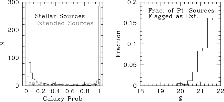
Figure 5: Left: Number of spectroscopically confirmed quasars classified by PHOTO as stellar (black) and as extended (grey) as a function of Bayesian galaxy probability (Scranton et al. 2002). Right: Fraction of point-like quasars (as determined by the Bayesian analysis) that are mis-classified by PHOTO as extended – as a function of magnitude.

Eddington bias is the distortion of the object number counts as a function of magnitude that occurs when photometric uncertainty causes errors in distributing sources into their proper magnitude bins. The relationship between the observed and actual differential number counts, $A(m)$, is given by Peterson (1997):

$$A(m)\approx A_{obs}(m)\left[1-\frac{1}{2}\left(\frac{\sigma\kappa}{\log e}\right)^{2}\right],$$ (22)

where $\sigma$ is the Gaussian error in the magnitude, $\kappa$ is defined by the integrated number counts relation $N(m)\propto C10^{\kappa m}$, and $\log A(m)=C+\kappa m$. If the product of the slope and the error ($\sigma\kappa$) increases with magnitude then the observed slope is steeper than the intrinsic slope; for decreasing $\sigma\kappa$ the observed slope is flatter than the intrinsic slope. For our sample the correction term in brackets above is $\geq 0.98$ for all magnitude bins, thus we have applied no correction for Eddington bias.

4.5 Morphology bias

Our sample includes objects that the SDSS photometric pipeline (PHOTO; Lupton et al. 2001) classifies as extended. The rationale for this decision is summarized in Figure 5 which shows that at the faintest limits of our survey, a significant fraction of point sources are mis-classified by the photometric pipeline as extended (assuming that the Bayesian analysis of Scranton et al. 2002 represents ground truth). The right-hand panel shows that this is a function of magnitude. The left-hand panel shows the Bayesian galaxy probability distribution for both point-like (stellar) and extended quasars as classified by PHOTO.

The inclusion of extended sources can lead to a bias. Specifically, since many of the Semester A targets have been observed as part of the 2QZ and since the 2QZ did not target extended sources, our new observations will be preferentially biased towards extended sources. Thus our corrections from the number of objects observed to the number of objects targeted may be skewed since it assumes that new observations will yield quasars at the same rate as old observations. However, we find that, although the contamination among extended sources is larger than for point sources, the shape of the corrections as a function of magnitude are not significantly different and thus our analysis of the shape of the QLF should not be adversely affected.

4.6 $g$ vs. $b_{J}$

To properly compare our 2SLAQ results to those of the 2QZ, we determine the relationship between the SDSS $g$ band and the $b_{J}$ band used by 2dF. Figure 6 shows the two transmission curves, which are quite similar. The $b_{J}$ curve was kindly provided by Paul Hewett (2004, priv. comm.). The $g$ curve is as taken from the SDSS web site – except that it has been converted from 1.3 to 1.0 airmasses (to match the $b_{J}$ curve). In Figure 7, we plot the $g-b_{J}$ magnitude difference versus $b_{J}$ for all of the 2QZ quasars in our sample. This plot shows that even considering the scatter in $g-b_{J}$, the $g$ band magnitude limits of our current sample completely encompass the 2QZ quasars.

Figure 6: UKST $b_{J}$ (P. Hewett 2004, private communication) and SDSS $g$ transmission curves for 1 airmass and normalized such that $\int S_{\lambda}\frac{d\lambda}{\lambda}=1$. Both curves are given in terms of detector quantum efficiency, which means the $g$ curve is shown as published, but the $b_{J}$ curve has been multiplied by wavelength.

Figure 7: $g-b_{J}$ magnitude differences versus $b_{J}$, where $g$ is from the SDSS and $b_{J}$ is from the 2QZ. The dotted lines show the $g$ magnitude limits of the 2SLAQ sample. The dashed lines show the $b_{J}$ magnitude limits of the 2QZ survey. The points connected by a solid line give the median $g-b_{J}$ as a function of $b_{J}$ in 0.5 mag bins. The median over all $b_{J}$ is $\langle\!g-b_{J}\!\rangle\;=-0.045$. Neither $g$ or $b_{J}$ are extinction corrected in this plot.

To convert $b_{J}$ to $g$ we simply compute the median $g-b_{J}$ difference, which is shown as a function of $b_{J}$ by points connected by solid lines in Figure 7. The median for the whole sample is $\langle\!g-b_{J}\!\rangle\;=-0.045$, with no significant dependence on $b_{J}$. Given the empirical similarity of the $g$ and $b_{J}$ magnitudes, and that the error in the computed median is of order the median itself, we have simply taken $b_{J}$ as an exact surrogate for $g$ in our comparison of the number counts and luminosity functions.

Much of the scatter between $b_{J}$ and $g$ is caused by variability in the $\geq$20 years between the epochs when the $b_{J}$ and $g$ data were taken – in contrast with the simultaneity of the SDSS 5-band imaging data. The scatter in $g-b_{J}$ is $\sigma_{g-b_{J}}=0.25$ at $b_{J}=18.475$ and $\sigma_{g-b_{J}}=0.38$ at $b_{J}=20.725$. At least $0.15$ mag of this error is due to photometric error in $b_{J}$ (Croom et al. 2004, Fig. 9); roughly $0.02$ and $0.035$ is due to photometric error in $g$. Thus, most of the scatter (roughly $\sigma\sim 0.2$) is thus caused by variability. Variability adds uncertainty to the magnitude distribution in the same manner as photometric errors and thus can modify the number counts through Eddington bias. Proper treatment of variability in light of quasar number counts is complicated, ideally using long terms averages of the quasars under consideration. However, we can estimate the effect that variability has on the slope of the number counts. If the variability amplitude is constant with magnitude, then variability will cause a slight flattening of the observed distribution due to the number counts being steeper at the bright end than at the faint end. For $\sigma_{\rm var}=0.2$, at $g\sim 18.5$ the number counts will be over-estimated by $\sim$8% and at $g\sim 20.7$ they will be over-estimated by $\sim$1%, which produces a negligible ($\sim$2%) change in slope over this range.

5 Number counts and luminosity function

5.1 Redshift and absolute magnitude distributions

Having discussed the various completeness corrections, we can now determine the number counts and luminosity function of our sample. Figure 8 shows the $M_{g}$ vs. redshift distribution of spectroscopically confirmed 2SLAQ, 2QZ and SDSS quasars in our sample – within the boundaries of new plate observations (105.7 deg²). The absolute $g$ magnitude, $M_{g}$, is computed using luminosity distances in the cosmology given in § 1 according to the prescription of Hogg (1999) and with the (albeit poor, but commonly used) assumption of a universal power-law continuum of $\alpha_{\nu}=-0.5$ ($f_{\nu}\propto\nu^{\alpha}$). Black, cyan and blue points represent new 2SLAQ quasars, previously confirmed 2QZ quasars and previously confirmed SDSS quasars, respectively. Dashed red lines at $g=18.0$ and 21.85 demarcate the $g$ magnitude boundaries of our sample. In addition we show the $g\sim b_{J}=20.85$ limit of the 2QZ survey. The histograms to the left and bottom of the figure show the one-dimensional distribution of sources in $M_{g}$ and redshift. We further overlay a grid which highlights the magnitude and redshift bins that were used in the construction of the Croom et al. (2004) QLF and will also be used for determining the binned 2SLAQ QLF.

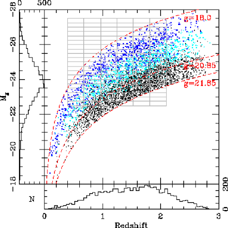
Figure 8: Absolute $g$ magnitude versus redshift for all confirmed quasars in our sample. Blue crosses are SDSS quasars, cyan crosses are 2QZ quasars, while black dots represents quasars confirmed by 2SLAQ. The bottom and side histograms show the 1D distributions of $M_{g}$ and redshift. The dashed red lines show the bright and faint magnitude limits of this survey ($g=18.0$ and $g=21.85$) and the approximate limit of the 2QZ survey in $g$ ($b_{J}=20.85$). The grid of grey lines outline the bins used for determining the quasar luminosity function.

5.2 Number counts

Figure 9 shows the differential number counts as a function of $g$ magnitude in bins of 0.25 mag, both corrected (solid circles) and uncorrected (open circles) for the various sources of incompleteness (error bars are Poisson). Number counts from 2QZ (Croom et al. 2004) are shown in red for comparison. This diagram only includes quasars with $M_{g}<-22.5$ and $0.4<z<2.1$.

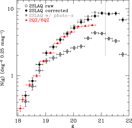
Figure 9: 2SLAQ number counts (black circles) compared to 2QZ number counts (red filled triangles) from Croom et al. (2004). The 2SLAQ number counts are given both as raw (i.e. observed; open circles) and corrected (filled circles) number counts. 2SLAQ number counts are also given (as grey circles) after including photometrically identified quasars (with photometric redshifts) from Richards et al. (2004). Quasars are restricted to those with $M_{g}<-22.5$ and $0.4<z<2.1$ (3889 quasars) for comparison with the 2QZ number counts. The dotted vertical line marks the dividing line between the 2SLAQ bright and faint samples.

From Figure 9 we see that to $g\sim 20.2$ the agreement between 2SLAQ and 2QZ is quite good, but there is a discrepancy between the two studies at the faint end: 2SLAQ suggesting a higher density of faint objects than 2QZ. We note that the shape of the distribution is clearly better fit by a double power law than a single power law (demonstrating the turnover in the distribution towards fainter quasars), but that the change in slope is more subtle than the distinctive “break” near $g\sim 19.5$ that is sometimes found in such analyses (e.g. Boyle et al. 1987). This behaviour is qualitatively consistent with that found by Wolf et al. (2003) from the COMBO-17 survey and is inconsistent with the single power-law form found in variability selected samples (e.g. Hawkins & Veron 1995, but see Ivezić et al. 2004).

We have shown (as open circles) the raw number counts to give the reader an idea of the absolute lower limits on the points and the size of the completeness corrections that have been applied. The coverage corrections are straightforward and should be fairly robust (perhaps less so in the 3 faintest bins due to the more restrictive selection criteria and larger photometric error). In fact, we could have simply corrected the effective area as a function of magnitude and shown the (more complete and much smoother) area-corrected raw counts. However, as we are splicing together three samples (SDSS, 2QZ, and 2SLAQ) to provide spectroscopic coverage of our targets, it seems appropriate to fully disclose the magnitude dependence of the coverage completeness within the 105.7 deg² area covered by the 2SLAQ plates. As a check on our correction terms, we have also matched our unobserved and unidentified objects to the photometric quasar candidate catalogue of Richards et al. (2004a), in attempt to “observe” a larger fraction of our quasar candidates (to $g<21$). The objects from Richards et al. (2004a) are expected to be 95 per cent accurate (averaged over all magnitdues) with respect to quasar classification, with 90 per cent having photometric redshifts correct to $|\Delta z|\pm 0.3$ for the redshift range considered here (Weinstein et al. 2004). The result of including these photometric identifications is shown by the grey points in Figure 9 and lends credence to the steeper faint-end number counts relations that we derive solely from our (completeness-corrected) spectroscopic sample. This comparison is meant purely as a sanity check. The differences between the spectroscopic (black cirles) and photometric (grey circles) number counts are consistent with the expected decrease in efficiency of the R04 photometric catalog with fainter magnitude, thus supporting the accuracy of our completeness determinations (and our corrected number counts).

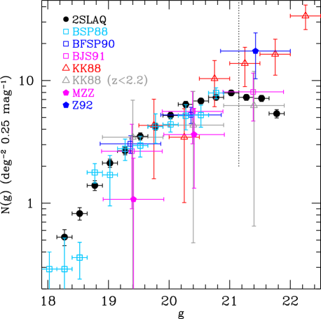
Figure 10: Comparison of 2SLAQ quasar number counts to previous deep samples. 2SLAQ quasars are limited to $M_{g}<-23$ and $0.6<z<2.2$ to mimic the exclusion of extended sources (which mostly have $z<0.6$ or $M_{g}>-23$). Open squares indicate points from Boyle and collaborators, specifically Boyle, Shanks & Peterson (1988) [cyan]; Boyle, Fong, Shanks & Peterson (1990) [blue]; Boyle, Jones & Shanks (1991; BSJ91) [magenta]. Open triangles refer to Koo & Kron (1988), where the red triangles are for $0.9<z<3.0$ and the grey triangles are for $z<2.2$ (and $z>0.9$) as given by Table 8 in BJS91. Filled magenta pentagons refer to Marano, Zamorani & Zitelli (1988), as given by Table 8 in BJS91. The filled blue pentagon is derived from Zitelli et al. (1992).

We further compare our results to a number of other samples of faint quasars that pre-date the 2QZ sample. This comparison is shown in Figure 10. Here we have restricted our sample to $0.6<z<2.2$ and $M_{g}<-23$ to best mimic the limits of these previous surveys which generally excluded extended sources (which typically have $z<0.6$ or $M_{g}>-23$). We specifically compare our 2SLAQ results to the samples of Boyle et al. (1988), Koo & Kron (1988), Marano, Zamorani & Zitelli (1988), Boyle et al. (1990), Boyle, Jones & Shanks (1991) and Zitelli et al. (1992), where Table 8 in Boyle et al. (1991) is the source of the Boyle et al. (1990), Zitelli et al. (1992), and Koo & Kron (1988) [$z<2.2$] points. The redshift ranges and magnitude calibrations between all of these samples do not match exactly, but they suffice to give the reader an idea of how our results compare with past work. In particular, in comparison with previous work we note that while the 2SLAQ data show an excess at $20<g<20.6$, it generally shows a deficit for $g>20.6$. The one exception is the faintest $z<2.2$ point from Koo & Kron (1988); however, that sample has a lower redshift limit of $z\sim 0.9$, whereas our sample extends to lower redshift. Overall, to the limit of our bright sample ($g<21.15$), our agreement with previous work is well within the errors. Fainter than $g=21.15$, if anything the 2SLAQ counts are deficient, but are still consistent considering the large coverage and spectroscopic completeness corrections at these limits. Figure 11 shows the cumulative 2SLAQ and 2QZ/6QZ quasar number counts. At the limit of the 2SLAQ survey, the cumulative counts compare well with the $J=22$ cumulative counts ($86.3\pm 16.5$) from Zitelli et al. (1992). The slope of the cumulative counts are given as 3-bin averages by the dashed lines and the numbers at the bottom of the plot. The brightest 2SLAQ points are unreliable as 2SLAQ does not include quasars brighter than $g=18$. The cumulative 2QZ/6QZ number counts gives a better idea of the slope at the bright end. Table 2 shows a comparison of the cumulative number counts predicted by the Boyle et al. (2000), Croom et al. (2004) and 2SLAQ best fit maximum likelihood parameterizations (assuming a double power-law and luminosity evolution characterized by a 2nd order polynomial) for $g>16.0$ and $0.3<z<2.2$.

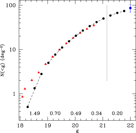
Figure 11: Cumulative 2SLAQ (black circles) and 2QZ (red triangles) as a function of $g$. The numbers at the bottom indicate the slope of the 3-bin least square fits shown by the series of dashed lines. Note that the bright limit of the 2SLAQ data is $g=18$ which causes a deficiency in the cumulative number counts at the bright end; at the faint end this lack of bright quasars makes little difference. While there is no strong characteristic break, the number counts clearly flatten with fainter magnitude. The blue pentagon shows the cumulative $J$-band number counts from Zitelli et al. (2002).

Table 2: Cumulative number count comparison. The cumulative number counts are shown for the Boyle et al. (2000), Croom et al. (2004) and 2SLAQ maximum likelihood parameterizations for $16<g<mag$ and $0.3<z<2.2$ in unit of counts per square degree.

$<mag$	Boyle00	Croom04	2SLAQ
20.0	15.87	17.50	18.96
20.5	26.99	28.27	31.09
21.0	41.68	40.22	47.79
21.5	59.45	52.01	69.13
22.0	78.88	62.46	93.77

5.3 Luminosity function

Figure 12 shows two determinations of luminosity function derived from our sample. We first use the Page & Carrera (2000) implementation of the $1/V$ method (Schmidt 1968; Avni & Bahcall 1980), which is shown by the points with error bars. This implementation corrects for incompleteness at both the bright and faint limits of the survey. These incomplete bins (those not filled in Figure 8) are shown as open rather than closed points to indicate that they have been corrected for partial coverage of the bin. However, we note that the Page & Carrera (2000) correction for incomplete bins is not fully accurate since the (relatively large) $z-M_{g}$ bins are not uniformly sampled, see Figure 8. The redshifts are the same as those in Figure 20 of Croom et al. (2004) for ease of comparison. The size of the redshifts bins is $\Delta z=0.283$ and the $z=1.39$ data are repeated as grey lines in each panel.

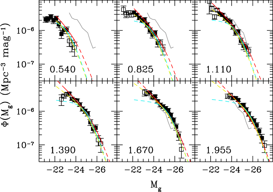
Figure 12: Faint quasar luminosity function for 2SLAQ quasars. Redshift bins are the same as for Croom et al. (2004). Open points are incomplete bins (see Fig. 8). Corrections for photometric, coverage and spectroscopic incompleteness have been applied. Only the quasars within the 41 new plate centers with $0.4<z<2.1$ are included. The $z=1.39$ data are repeated as grey curves in each panel for comparison. Best fit models (luminosity evolution characterized by a 2nd order polynomial in redshift) are shown from Boyle et al. (2000) [yellow], Croom et al. 2004 [cyan] and this work (red) as solid and dashed lines. The dashed parts of the best fit lines indicate where the fits have been extrapolated beyond the data. The faint quasar data suggest a steeper slope than the Croom et al. (2004) models.

We next give the luminosity function as derived from a maximum likelihood analysis; these are plotted as dashed/solid lines, the dashed part indicating extrapolation beyond the data used for the fit. The cyan lines show the best fit double power-law model (see below) from row 1 in Table 6 of Croom et al. (2004), which provide a poor fit at the faint end. The yellow lines show a similar model from row 1 in Table 3 of Boyle et al. (2000) (corrected to our cosmology), which has a steeper faint-end slope. Our own fit is shown in red and was derived as described below.

We have assumed a luminosity function in the standard form of a double-power law (Peterson 1997; Croom et al. 2004)

$$\Phi(L_{g},z)=\frac{\Phi(L_{g}^{*})/L_{g}^{*}}{(L_{g}/L_{g}^{*})^{-\alpha}+(L_{g}/L_{g}^{*})^{-\beta}},$$ (23)

or

$$\Phi(M_{g},z)=\frac{\Phi(M_{g}^{*})}{10^{0.4(\alpha+1)(M_{g}-M_{g}^{*})}+10^{0.4(\beta+1)(M_{g}-M_{g}^{*})}}.$$ (24)

We assume that the evolution with redshift is characterized by pure luminosity evolution (individual quasars getting fainter from $z=2$ to today), with the dependence of the characteristic luminosity described by a 2nd-order polynomial in redshift as in Croom et al. (2004) where

$$M_{g}^{*}(z)=M_{g}^{*}(0)-2.5(k_{1}z+k_{2}z^{2}).$$ (25)

Note that this form assumes symmetric redshift evolution about the peak. This assumption is appropriate for UVX samples such as this one, but will break down for samples that extend to higher redshifts (e.g. Richards et al. 2005).

We compute the maximum likelihood solution via Powell’s method (Press et al. 1992) using the form given by Fan et al. (2001b). We first attempt to determine the best fit parameters by allowing all of the parameters to vary. The resulting parameters are given in the last row of Table 2 and the fit is given by the red line in Figure 12. Due to the large incompleteness in our last magnitude bin, we have performed these fits to a limiting magnitude of $g<21.65$ rather than $g<21.85$. The errors on the parameters are $\sigma_{\alpha}=0.2$, $\sigma_{\beta}=0.03$, $\sigma_{M^{*}}=0.09$, $\sigma_{k1}=0.02$, $\sigma_{k2}=0.01$.

Since there are relatively few bright quasars in our sample to tie down the bright end slope, we have also attempted to fix all of the parameters except for the faint end slope ($\beta$) and the normalization to those found by Croom et al. (2004), specifically $\alpha=-3.31$, $M_{g}^{*}=-21.61+5\log h_{70}$, $k_{1}=1.39$, and $k_{2}=-0.29$. The resulting faint end slope is then $\beta=-1.45\pm 0.03$ (with $\Phi^{*}=1.83\times 10^{-6}h_{70}^{3}$ Mpc^-3 mag^-1). For both of these fits, a $\chi^{2}$ comparison of this model to the $1/V_{a}$ data is formally rejected; see Table 2. We also note that there is apparently substantial covariance between the parameters. For example, there is a significant difference in the faint end slopes of the Boyle et al. (2000) and Croom et al. (2004) analysis (as shown by the cyan and yellow lines in Fig. 12), yet there is only a 1 per cent difference in the total expected counts to the limiting magnitude of the 2QZ survey ($b_{J}=20.85$). To the fainter limit of our survey, we find that the final 2QZ parameterization (Croom et al. 2004) significantly underpredicts (by 32 per cent) the total number of quasars to $g<21.65$, while the Boyle et al. (2000) parameters yield a much better fit to the 2SLAQ data (see Fig. 12 and Table 2). The deviation from the best fit 2QZ model can be seen better in the left-hand panel of Figure 13 where we have normalized our derived values by the best fit polynomial evolution model from Croom et al. (2004). The right hand panel is similar except that the data have all been normalized to our $z=1.39$ model in order to better show the redshift evolution of the quasars. All of the above suggests that the adopted parameterization is not the optimal one; however, it still has considerable utility in terms of predicting counts of faint quasars and as an input for theoretical models.

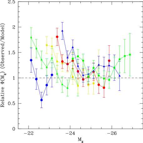
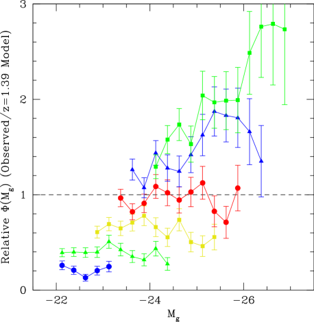
Figure 13: Left: Ratio of luminosity function from Fig. 12 to the polynomial evolution models from Croom et al. (2004) . Colours and points are as in Figure 20 of Croom et al. (2004) , specifically blue circles, green triangles, yellow squares, red circles, blue triangles, and green squares, corresponding to redshifts 0.54, 0.825, 1.11, 1.39, 1.67, and 1.955, respectively. Note the deviation from unity at the faint end in each redshift bin. Right: The ratio of the luminosity function to our $z=1.39$ maximum likelihood model.

Table 3: Summary of maximum likelihood fits for the parameterization adopted for the 2QZ analysis (double power-law with luminosity evolution parameterized as a 2nd order polynomial in redshift) and our adopted cosmology (§ 1). The redshift limits is $0.4<z<2.1$, and objects must be brighter then $M<-22.5$. $N_{Q}$ indicates the number of quasars per square degree expected for $18.0<g<21.65$.

Sample	$\alpha$	$\beta$	$M^{*}$	$k_{1}$	$k_{2}$	$\Phi^{*}$	$N_{Q}$	$\chi^{2}$	$\nu$	$P_{\chi^{2}}$
Boyle et al. (2000)	$-3.41$	$-1.58$	$-21.92$	1.36	$-0.27$	9.88e-7	66.8
Croom et al. (2004)	$-3.31$	$-1.09$	$-21.61$	1.39	$-0.29$	1.67e-6	54.4
2SLAQ + Croom et al. (2004)	$-3.31$	$-1.45$	$-21.61$	1.39	$-0.29$	1.83e-6	83.8	161.5	55	2.1e-12
2SLAQ only	$-3.28$	$-1.78$	$-22.68$	1.37	$-0.32$	5.96e-7	79.8	149.0	51	1.5e-11

We have also attempted to use the parameterizations of the luminosity function that were used by Wolf et al. (2003) since our data, like that of COMBO-17, appears to show less of a break in the luminosity function than previous work. The best fit forms and parameters from Wolf et al. (2003) match the 2SLAQ data over a limited range in redshift and absolute magnitude, but these fits do not agree with the 2SLAQ data at the bright end and for lower redshifts. We were also unable to derive better fits to the 2SLAQ data using such parameterizations, likely because of the lack of dynamic range at the bright end of the distribution. However, it is clear that other parameterizations, like those adopted by COMBO-17, are worth pursuing.

5.4 X-ray comparison

We can test the robustness of the faint end of the 2SLAQ luminosity function by comparing to quasar luminosity functions derived from X-ray selected samples which are thought to suffer less incompleteness as a result of the dust-penetrating nature of X-ray photons. In Figure 14 we compare the $z=0.825$ and $z=1.67$ redshift bins from Figure 12 to Croom et al. (2004) and two quasar luminosity functions derived from hard X-ray surveys (Ueda et al. 2003; Barger et al. 2005).

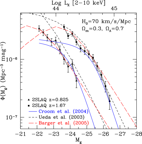
Figure 14: Comparison of the 2SLAQ optical quasar luminosity function with X-ray quasar luminosity functions from the literature. Shown are the $z=0.825$ (triangles) and $z=1.67$ (squares) QLF from 2SLAQ and the best fit models for those redshifts from three other papers. The models are from Croom et al. (2004) (blue solid line), Ueda et al. (2003) (dashed black line) and Barger et al. (2005) (red long dashed line).

In these comparisons, we have converted between $M_{g}$ and $\log(L[2-10{\rm keV}])$ as follows. First we take our K-corrected $M_{g}$ and convert it to (rest-frame) $\log(L_{g}[{\rm erg\,s^{-1}\,cm^{-2}\,Hz^{-1}}])$ as prescribed by the definition of an AB (Oke & Gunn 1983) magnitude and an absolute magnitude (with an assumed distance of 10 pc)

$$\log(L_{g})=-0.4(M_{g}-5+48.6)+\log(4\pi)+2\log(3.086\times 10^{18}).$$ (26)

Next we assume a power-law spectral index of $\alpha_{\nu}=-0.5$ to convert from rest-frame $g$ (4669Å) to rest-frame 2500Å according to

$$\log(L_{2500})=\log(L_{g})-0.5\log(4669/2500).$$ (27)

We then extrapolate to $\log(L_{2keV})$ assuming a luminosity dependent 2500Å to 2 keV slope, $\alpha_{ox}$, (Vignali, Brandt & Schneider 2003):

$$\alpha_{ox}=-0.11\log(L_{2500})+1.85$$ (28)

and

$$\log(L_{2keV})=\log(L_{2500})+\alpha_{ox}\log\left(\frac{\nu_{2keV}}{\nu_{2500}}\right).$$ (29)

(Using the revised $\alpha_{ox}-L_{2500}$ relationship from Strateva et al. 2005 yields somewhat fainter X-ray luminosities [$\sim 0.15$ dex] at the bright end of our sample and would slightly flatten the X-ray QLFs in Fig. 14.) Finally, we compute a 2–10 keV luminosity by integrating over the 2–10 keV range assuming a photon index of $\Gamma=1.9$ ($\alpha_{x}=-0.9$). For comparison with Ueda et al. (2003) we further correct for the fraction of X-ray type II AGN according to their Figure 8 and an optical type II fraction of 0.5, which is roughly consistent with their Figure 9. In our comparison with the broad-line AGN luminosity function of Barger et al. (2005), we have treated their parameterization as if it were for a 2–10 keV luminosity rather than a 2–8 keV luminosity (since we are primarily concerned with the comparisons of the QLF slope), and we have applied a correction factor of $0.5$ in the overall normalization. Furthermore, our comparison with Barger et al. (2005) differs somewhat from their comparison with Croom et al. (2004) in that Barger et al. (2005) converted the optical and X-ray luminosities to bolometric luminosities in a manner which assumes a constant $\alpha_{ox}$, whereas we assumed the luminosity-dependent $\alpha_{ox}$ given above. For both comparisons with X-ray QLFs we have converted the parameterizations to the cosmology adopted herein.

For the sake of facilitating the comparison of optical QLFs to X-ray QLFs, we note that, in the syntax used by Ueda et al. (2003) in their Equation 6 (and similar notation used by Barger et al. 2005, Equation 1) $\phi_{M}=A/2.5$, $\alpha=-(\gamma_{1}+1)$, and $\beta=-(\gamma_{2}+1)$, where $\phi_{M}$, $\alpha$, and $\beta$ are defined as in Peterson (1997), Equation 11.33 (and similarly by Croom et al. 2004, Equation 11).

In each case, the X-ray luminosity functions show less curvature in the faintest 2SLAQ bins than does the best fit model from 2QZ. This comparison is not meant to be strictly quantitative since X-ray selected samples are more sensitive to obscured quasars and the conversion between $M_{B}$ and $L_{X}$ involves a number of tenuous assumptions. However, these comparisons confirm that the steeper 2SLAQ faint end slope, while based on large correction factors, is quite reasonable. In particular, the agreement with the results of Barger et al. (2005) is remarkable.

6 Discussion and Conclusions

We have compiled a sample of 5645 quasars with $18.0<g<21.85$ and $z<3$ using imaging data from the SDSS and the spectra from the 2dF facility at the AAT. We find a clear turnover in the optical number counts; a single power-law is not a good fit over the magnitude range sampled. For $20<g<20.6$, the 2SLAQ number counts show a slight (but statistically insignificant) excess over previous surveys, but the cumulative number counts are roughly consistent with the faintest surveys to 22nd magnitude.

In terms of the luminosity function, we find good agreement with the 2QZ results from Croom et al. (2004) at the bright end, but the faint end 2SLAQ data require a steeper slope (higher density of quasars) than the 2QZ results from Croom et al. (2004). The previous 2QZ results from Boyle et al. (2000) agree significantly better with 2SLAQ at the faint end. The lack of a well defined characteristic luminosity and covariance between the maximum likelihood parameters can explain the good bright-end agreement between the parameterizations studied and the faint-end disagreement between 2SLAQ and the final 2QZ results Croom et al. (2004). Comparing to type I quasar luminosity functions derived from X-ray samples suggests that the slope of the faint end of the 2SLAQ QLF is more accurate than the extrapolated faint end slope of Croom et al. (2004).

An understanding of the quasar luminosity function is an important ingredient for many different types of extragalactic investigations. In particular, as has been stressed by those working with X-ray selected samples, investigations that depend on the optical QLF explicitly may need to be reconsidered as a result of recent revisions in the luminosity function of unobscured AGNs (not to mention obscured AGNs). Many investigations have an explicit dependence on the optical QLF, for example Bianchi, Cristiani & Kim (2001) in their analysis of the UV background; Hamilton, Casertano & Turnshek (2002) in their estimate of the quasar host galaxy luminosity function; Yu & Tremaine (2002) in their investigation of the growth of black holes; Croom et al. (2002) and Wake et al. (2004) regarding the clustering of AGN; Oguri (2003) in his determination of the expected number of lensed quasars; Richards et al. (2004b) in their assessment of the lensing probability of the most luminous high-redshift quasars; and Fan et al. (2001a) in terms of the evolution of quasars from $z=0$ to $z=6$. The QLF has taken on even greater importance in recent years with the realization that most massive galaxies host supermassive black holes, the correlation between black hole mass and stellar velocity dispersion (e.g. Magorrian et al. 1998; Ferrarese & Merritt 2000; Gebhardt et al. 2000), and the possibility that feedback from quasars may play a role in the evolution of galaxies in general (e.g. Begelman 2004). In particular, models like those of Kauffmann & Haehnelt (2000), Wyithe & Loeb (2002), and others that attempt to explain the evolution of galaxies and quasars, rely on comparison with accurate observational determinations of the QLF.

In fact, although the optical QLF presented herein is arguably the most robust determination to date for a large optically selected sample, for many applications an X-ray or far-IR QLF is more appropriate. That said, the luminosity function of optically selected quasars will remain an important tool for extragalactic astronomy. The primary reason for this is the sheer size of the optical quasar sample (likely over 300,000 in the current SDSS imaging data alone; Richards et al. 2004a). While the deepest X-ray surveys may uncover thousands of AGNs per square degree, they do so over only a fraction of a square degree and the sum total area of the sky covered by both Chandra and XMM-Newton is unlikely to ever exceed even 1 per cent. IR surveys with Spitzer will cover a somewhat larger area than X-ray surveys, but not at nearly the same space density as in the X-ray or with nearly the same total number as in the shallower, but much wider optical surveys. Thus, this sample of faint quasars and the luminosity function derived from it will continue to provide important inputs to future extragalactic investigations such as the Dark Energy Survey (DES) and the Large Synoptic Survey Telescope (LSST).

References

- [Abazajian, Adelman-McCarthy, Agüeros, Allam, Anderson, Annis, Bahcall, Baldry, Bastian, Berlind, Bernardi, Blanton, Blythe, Bochanski, Boroski, Brewington, Briggs, Brinkmann, Brunner, Budavári, Carey, Carr, Castander, Chiu, Collinge, Connolly, Covey, Csabai, Dalcanton, Dodelson, Doi, Dong, Eisenstein, Evans, Fan, Feldman, Finkbeiner, Friedman, Frieman, Fukugita, Gal, Gillespie, Glazebrook, Gonzalez, Gray, Grebel, Grodnicki, Gunn, Gurbani, Hall, Hao, Harbeck, Harris, Harris, Harvanek, Hawley, Heckman, Helmboldt, Hendry, Hennessy, Hindsley, Hogg, Holmgren, Holtzman, Homer, Hui, Ichikawa, Ichikawa, Inkmann, Ivezić, Jester, Johnston, Jordan, Jordan, Jorgensen, Jurić, Kauffmann, Kent, Kleinman, Knapp, Kniazev, Kron, Krzesiński, Kunszt, Kuropatkin, Lamb, Lampeitl, Laubscher, Lee, Leger, Li, Lidz, Lin, Loh, Long, Loveday, Lupton, Malik, Margon, McGehee, McKay, Meiksin, Miknaitis, Moorthy, Munn, Murphy, Nakajima, Narayanan, Nash, Neilsen, Newberg, Newman, Nichol, Nicinski, Nieto-Santisteban, Nitta, Odenkirchen, Okamura, Ostriker, Owen, Padmanabhan, Peoples, Pier, Pindor, Pope, Quinn, Rafikov, Raymond, Richards, Richmond, Rix, Rockosi, Schaye, Schlegel, Schneider, Schroeder, Scranton, Sekiguchi, Seljak, Sergey, Sesar, Sheldon, Shimasaku, Siegmund, Silvestri, Sinisgalli, Sirko, Smith, Smolčić, Snedden, Stebbins, Steinhardt, Stinson, Stoughton, Strateva, Strauss, SubbaRao, Szalay, Szapudi, Szkody, Tasca, Tegmark, Thakar, Tremonti, Tucker, Uomoto, Vanden Berk, Vandenberg, Vogeley, Voges, Vogt, Walkowicz, Weinberg, West, White, Wilhite, Willman, Xu, Yanny, Yarger, Yasuda, Yip, Yocum, York, Zakamska, Zehavi, Zheng, Zibetti, & Zucker 2003] Abazajian, K., Adelman-McCarthy, J. K., Agüeros, M. A., Allam, S. S., et al. 2003, AJ, 126, 2081
- [Avni & Bahcall 1980] Avni, Y. & Bahcall, J. N. 1980, ApJ, 235, 694
- [Barger et al. 2005] Barger et al. 2005, accepted (astro-ph/0410527)
- [Begelman 2004] Begelman, M. C. 2004, in Coevolution of Black Holes and Galaxies, 375
- [Bianchi, Cristiani, & Kim 2001] Bianchi, S., Cristiani, S., & Kim, T.-S. 2001, A&A, 376, 1
- [Blanton, Lin, Lupton, Maley, Young, Zehavi, & Loveday 2003] Blanton, M. R., Lin, H., Lupton, R. H., Maley, F. M., Young, N., Zehavi, I., & Loveday, J. 2003, AJ, 125, 2276
- [Boyle, Fong, Shanks, & Peterson 1987] Boyle, B. J., Fong, R., Shanks, T., & Peterson, B. A. 1987, MNRAS, 227, 717
- [Boyle, Fong, Shanks, & Peterson 1990] —. 1990, MNRAS, 243, 1
- [Boyle, Jones, & Shanks 1991] Boyle, B. J., Jones, L. R., & Shanks, T. 1991, MNRAS, 251, 482
- [Boyle, Shanks, Croom, Smith, Miller, Loaring, & Heymans 2000] Boyle, B. J., Shanks, T., Croom, S. M., Smith, R. J., Miller, L., Loaring, N., & Heymans, C. 2000, MNRAS, 317, 1014
- [Boyle, Shanks, & Peterson 1988] Boyle, B. J., Shanks, T., & Peterson, B. A. 1988, MNRAS, 235, 935
- [Cannon et al. 2003] Cannon et al. 2003, AAO Newsletter, 103, 8
- [Cannon et al. 2005] —. 2005, in prep.
- [Croom, Boyle, Loaring, Miller, Outram, Shanks, & Smith 2002] Croom, S. M., Boyle, B. J., Loaring, N. S., Miller, L., Outram, P. J., Shanks, T., & Smith, R. J. 2002, MNRAS, 335, 459
- [Croom, Smith, Boyle, Shanks, Loaring, Miller, & Lewis 2001] Croom, S. M., Smith, R. J., Boyle, B. J., Shanks, T., Loaring, N. S., Miller, L., & Lewis, I. J. 2001, MNRAS, 322, L29
- [Croom, Smith, Boyle, Shanks, Miller, Outram, & Loaring 2004] Croom, S. M., Smith, R. J., Boyle, B. J., Shanks, T., Miller, L., Outram, P. J., & Loaring, N. S. 2004, MNRAS, 349, 1397
- [Fan 1999] Fan, X. 1999, AJ, 117, 2528
- [Fan, Narayanan, Lupton, Strauss, Knapp, Becker, White, Pentericci, Leggett, Haiman, Gunn, Ivezić, Schneider, Anderson, Brinkmann, Bahcall, Connolly, Csabai, Doi, Fukugita, Geballe, Grebel, Harbeck, Hennessy, Lamb, Miknaitis, Munn, Nichol, Okamura, Pier, Prada, Richards, Szalay, & York 2001a] Fan, X., Narayanan, V. K., Lupton, R. H., Strauss, M. A., et al. 2001a, AJ, 122, 2833
- [Fan, Strauss, Schneider, Gunn, Lupton, Becker, Davis, Newman, Richards, White, Anderson, Annis, Bahcall, Brunner, Csabai, Hennessy, Hindsley, Fukugita, Kunszt, Ivezić, Knapp, McKay, Munn, Pier, Szalay, & York 2001b] Fan, X., Strauss, M. A., Schneider, D. P., Gunn, J. E., et al. 2001b, AJ, 121, 54
- [Ferrarese & Merritt 2000] Ferrarese, L. & Merritt, D. 2000, ApJ, 539, L9
- [Fukugita, Ichikawa, Gunn, Doi, Shimasaku, & Schneider 1996] Fukugita, M., Ichikawa, T., Gunn, J. E., Doi, M., Shimasaku, K., & Schneider, D. P. 1996, AJ, 111, 1748
- [Gebhardt, Bender, Bower, Dressler, Faber, Filippenko, Green, Grillmair, Ho, Kormendy, Lauer, Magorrian, Pinkney, Richstone, & Tremaine 2000] Gebhardt, K., Bender, R., Bower, G., Dressler, A., et al. 2000, ApJ, 539, L13
- [Gunn, Carr, Rockosi, Sekiguchi, Berry, Elms, de Haas, Ivezić , Knapp, Lupton, Pauls, Simcoe, Hirsch, Sanford, Wang, York, Harris, Annis, Bartozek, Boroski, Bakken, Haldeman, Kent, Holm, Holmgren, Petravick, Prosapio, Rechenmacher, Doi, Fukugita, Shimasaku, Okada, Hull, Siegmund, Mannery, Blouke, Heidtman, Schneider, Lucinio, & Brinkman 1998] Gunn, J. E., Carr, M., Rockosi, C., Sekiguchi, M., et al. 1998, AJ, 116, 3040
- [Hamilton, Casertano, & Turnshek 2002] Hamilton, T. S., Casertano, S., & Turnshek, D. A. 2002, ApJ, 576, 61
- [Hawkins & Veron 1995] Hawkins, M. R. S. & Veron, P. 1995, MNRAS, 275, 1102
- [Hewett, Foltz, & Chaffee 1993] Hewett, P. C., Foltz, C. B., & Chaffee, F. H. 1993, ApJ, 406, L43
- [Hogg 1999] Hogg, D. W. 1999, preprint, astro-ph/9905116
- [Hogg, Finkbeiner, Schlegel, & Gunn 2001] Hogg, D. W., Finkbeiner, D. P., Schlegel, D. J., & Gunn, J. E. 2001, AJ, 122, 2129
- [Kauffmann & Haehnelt 2000] Kauffmann, G. & Haehnelt, M. 2000, MNRAS, 311, 576
- [Kennefick, Djorgovski, & de Carvalho 1995] Kennefick, J. D., Djorgovski, S. G., & de Carvalho, R. R. 1995, AJ, 110, 2553
- [Koo & Kron 1988] Koo, D. C. & Kron, R. G. 1988, ApJ, 325, 92
- [Lewis, Cannon, Taylor, Glazebrook, Bailey, Baldry, Barton, Bridges, Dalton, Farrell, Gray, Lankshear, McCowage, Parry, Sharples, Shortridge, Smith, Stevenson, Straede, Waller, Whittard, Wilcox, & Willis 2002] Lewis, I. J., Cannon, R. D., Taylor, K., Glazebrook, K., et al. 2002, MNRAS, 333, 279
- [Lupton, Gunn, Ivezić, Knapp, Kent, & Yasuda 2001] Lupton, R. H., Gunn, J. E., Ivezić, Z., Knapp, G. R., Kent, S., & Yasuda, N. 2001, in ASP Conf. Ser. 238: Astronomical Data Analysis Software and Systems X, Vol. 10, 269
- [Lupton, Gunn, & Szalay 1999] Lupton, R. H., Gunn, J. E., & Szalay, A. S. 1999, AJ, 118, 1406
- [Magorrian, Tremaine, Richstone, Bender, Bower, Dressler, Faber, Gebhardt, Green, Grillmair, Kormendy, & Lauer 1998] Magorrian, J., Tremaine, S., Richstone, D., Bender, R., et al. 1998, AJ, 115, 2285
- [Marano, Zamorani, & Zitelli 1988] Marano, B., Zamorani, G., & Zitelli, V. 1988, MNRAS, 232, 111
- [Oguri 2003] Oguri, M. 2003, MNRAS, 339, L23
- [Oke & Gunn 1983] Oke, J. B. & Gunn, J. E. 1983, ApJ, 266, 713
- [Padmanabhan et al. 2004] Padmanabhan et al. 2004, submitted (astro-ph/0407594)
- [Page & Carrera 2000] Page, M. J. & Carrera, F. J. 2000, MNRAS, 311, 433
- [Peterson 1997] Peterson, B. M. 1997, An introduction to active galactic nuclei (Publisher: Cambridge, New York Cambridge University Press)
- [Pier, Munn, Hindsley, Hennessy, Kent, Lupton, & Ivezić 2003] Pier, J. R., Munn, J. A., Hindsley, R. B., Hennessy, G. S., Kent, S. M., Lupton, R. H., & Ivezić, Ž. 2003, AJ, 125, 1559
- [Press, Teukolsky, Vetterling, & Flannery 1992] Press, W. H., Teukolsky, S. A., Vetterling, W. T., & Flannery, B. P. 1992, Numerical recipes in C. The art of scientific computing (Cambridge: University Press, —c1992, 2nd ed.)
- [Richards, Fan, Newberg, Strauss, Vanden Berk, Schneider, Yanny, Boucher, Burles, Frieman, Gunn, Hall, Ivezić, Kent, Loveday, Lupton, Rockosi, Schlegel, Stoughton, SubbaRao, & York 2002] Richards, G. T., Fan, X., Newberg, H. J., Strauss, M. A., et al. 2002, AJ, 123, 2945
- [Richards, Fan, Schneider, Vanden Berk, Strauss, York, Anderson, Anderson, Annis, Bahcall, Bernardi, Briggs, Brinkmann, Brunner, Burles, Carey, Castander, Connolly, Crocker, Csabai, Doi, Finkbeiner, Friedman, Frieman, Fukugita, Gunn, Hindsley, Ivezić, Kent, Knapp, Lamb, Leger, Long, Loveday, Lupton, McKay, Meiksin, Merrelli, Munn, Newberg, Newcomb, Nichol, Owen, Pier, Pope, Richmond, Rockosi, Schlegel, Siegmund, Smee, Snir, Stoughton, Stubbs, SubbaRao, Szalay, Szokoly, Tremonti, Uomoto, Waddell, Yanny, & Zheng 2001] Richards, G. T., Fan, X., Schneider, D. P., Vanden Berk, D. E., et al. 2001, AJ, 121, 2308
- [Richards, Nichol, Gray, Brunner, Lupton, Vanden Berk, Chong, Weinstein, Schneider, Anderson, Munn, Harris, Strauss, Fan, Gunn, Ivezić, York, Brinkmann, & Moore 2004a] Richards, G. T., Nichol, R. C., Gray, A. G., Brunner, R. J., et al. 2004a, ApJS, 155, 257
- [Richards, Strauss, Pindor, Haiman, Fan, Eisenstein, Schneider, Bahcall, Brinkmann, & Brunner 2004b] Richards, G. T., Strauss, M. A., Pindor, B., Haiman, Z., et al. 2004b, AJ, 127, 1305
- [Richards et al. 2005] Richards et al. 2005, in preparation
- [Schlegel, Finkbeiner, & Davis 1998] Schlegel, D. J., Finkbeiner, D. P., & Davis, M. 1998, ApJ, 500, 525
- [Schmidt 1968] Schmidt, M. 1968, ApJ, 151, 393
- [Schmidt & Green 1983] Schmidt, M. & Green, R. F. 1983, ApJ, 269, 352
- [Schmidt, Schneider, & Gunn 1995] Schmidt, M., Schneider, D. P., & Gunn, J. E. 1995, AJ, 110, 68
- [Schneider, Fan, Hall, Jester, Richards, Stoughton, Strauss, SubbaRao, Vanden Berk, Anderson, Brandt, Gunn, Gray, Trump, Voges, Yanny, Bahcall, Blanton, Boroski, Brinkmann, Brunner, Burles, Castander, Doi, Eisenstein, Frieman, Fukugita, Heckman, Hennessy, Ivezić, Kent, Knapp, Lamb, Lee, Loveday, Lupton, Margon, Meiksin, Munn, Newberg, Nichol, Niederste-Ostholt, Pier, Richmond, Rockosi, Saxe, Schlegel, Szalay, Thakar, Uomoto, & York 2003] Schneider, D. P., Fan, X., Hall, P. B., Jester, S., et al. 2003, AJ, 126, 2579
- [Schneider, Fan, Hall, Jester, Richards, Stoughton, Strauss, SubbaRao, Vanden Berk, Anderson, Brandt, Gunn, Gray, Trump, Voges, Yanny, Bahcall, Blanton, & York 2005] Schneider, D. P., Fan, X., Hall, P. B., Jester, S., et al. 2005, AJ, submitted
- [Scranton, Johnston, Dodelson, Frieman, Connolly, Eisenstein, Gunn, Hui, Jain, Kent, Loveday, Narayanan, Nichol, O’Connell, Scoccimarro, Sheth, Stebbins, Strauss, Szalay, Szapudi, Tegmark, Vogeley, Zehavi, Annis, Bahcall, Brinkman, Csabai, Hindsley, Ivezic, Kim, Knapp, Lamb, Lee, Lupton, McKay, Munn, Peoples, Pier, Richards, Rockosi, Schlegel, Schneider, Stoughton, Tucker, Yanny, & York 2002] Scranton, R., Johnston, D., Dodelson, S., Frieman, J. A., et al. 2002, ApJ, 579, 48
- [Smith, Tucker, Kent, Richmond, Fukugita, Ichikawa, Ichikawa, Jorgensen, Uomoto, Gunn, Hamabe, Watanabe, Tolea, Henden, Annis, Pier, McKay, Brinkmann, Chen, Holtzman, Shimasaku, & York 2002] Smith, J. A., Tucker, D. L., Kent, S., Richmond, M. W., et al. 2002, AJ, 123, 2121
- [Spergel, Verde, Peiris, Komatsu, Nolta, Bennett, Halpern, Hinshaw, Jarosik, Kogut, Limon, Meyer, Page, Tucker, Weiland, Wollack, & Wright 2003] Spergel, D. N., Verde, L., Peiris, H. V., Komatsu, E., et al. 2003, ApJS, 148, 175
- [Stoughton, Lupton, Bernardi, Blanton, Burles, Castander, Connolly, Eisenstein, Frieman, Hennessy, Hindsley, Ivezić, Kent, Kunszt, Lee, Meiksin, Munn, Newberg, Nichol, Nicinski, Pier, Richards, Richmond, Schlegel, Smith, Strauss, SubbaRao, Szalay, Thakar, Tucker, Vanden Berk, Yanny, Adelman, Anderson, Anderson, Annis, Bahcall, Bakken, Bartelmann, Bastian, Bauer, Berman, Böhringer, Boroski, Bracker, Briegel, Briggs, Brinkmann, Brunner, Carey, Carr, Chen, Christian, Colestock, Crocker, Csabai, Czarapata, Dalcanton, Davidsen, Davis, Dehnen, Dodelson, Doi, Dombeck, Donahue, Ellman, Elms, Evans, Eyer, Fan, Federwitz, Friedman, Fukugita, Gal, Gillespie, Glazebrook, Gray, Grebel, Greenawalt, Greene, Gunn, de Haas, Haiman, Haldeman, Hall, Hamabe, Hansen, Harris, Harris, Harvanek, Hawley, Hayes, Heckman, Helmi, Henden, Hogan, Hogg, Holmgren, Holtzman, Huang, Hull, Ichikawa, Ichikawa, Johnston, Kauffmann, Kim, Kimball, Kinney, Klaene, Kleinman, Klypin, Knapp, Korienek, Krolik, Kron, Krzesiński, Lamb, Leger, Limmongkol, Lindenmeyer, Long, Loomis, Loveday, MacKinnon, Mannery, Mantsch, Margon, McGehee, McKay, McLean, Menou, Merelli, Mo, Monet, Nakamura, Narayanan, Nash, Neilsen, Newman, Nitta, Odenkirchen, Okada, Okamura, Ostriker, Owen, Pauls, Peoples, Peterson, Petravick, Pope, Pordes, Postman, Prosapio, Quinn, Rechenmacher, Rivetta, Rix, Rockosi, Rosner, Ruthmansdorfer, Sandford, Schneider, Scranton, Sekiguchi, Sergey, Sheth, Shimasaku, Smee, Snedden, Stebbins, Stubbs, Szapudi, Szkody, Szokoly, Tabachnik, Tsvetanov, Uomoto, Vogeley, Voges, Waddell, Walterbos, Wang, Watanabe, Weinberg, White, White, Wilhite, Wolfe, Yasuda, York, Zehavi, & Zheng 2002] Stoughton, C., Lupton, R. H., Bernardi, M., Blanton, M. R., et al. 2002, AJ, 123, 485
- [Strateva et al.(2005)] Strateva, I., Brandt, N., Schneider, D., Vanden Berk, D., & Vignali, C. 2005, ArXiv Astrophysics e-prints, astro-ph/0503009
- [Telfer, Zheng, Kriss, & Davidsen 2002] Telfer, R. C., Zheng, W., Kriss, G. A., & Davidsen, A. F. 2002, ApJ, 565, 773
- [Ueda, Akiyama, Ohta, & Miyaji 2003] Ueda, Y., Akiyama, M., Ohta, K., & Miyaji, T. 2003, ApJ, 598, 886
- [Vanden Berk, Richards, Bauer, Strauss, Schneider, Heckman, York, Hall, Fan, Knapp, Anderson, Annis, Bahcall, Bernardi, Briggs, Brinkmann, Brunner, Burles, Carey, Castander, Connolly, Crocker, Csabai, Doi, Finkbeiner, Friedman, Frieman, Fukugita, Gunn, Hennessy, Ivezić, Kent, Kunszt, Lamb, Leger, Long, Loveday, Lupton, Meiksin, Merelli, Munn, Newberg, Newcomb, Nichol, Owen, Pier, Pope, Rockosi, Schlegel, Siegmund, Smee, Snir, Stoughton, Stubbs, SubbaRao, Szalay, Szokoly, Tremonti, Uomoto, Waddell, Yanny, & Zheng 2001] Vanden Berk, D. E., Richards, G. T., Bauer, A., Strauss, M. A., et al. 2001, AJ, 122, 549
- [Vanden Berk et al. 2005] Vanden Berk et al. 2005, in press
- [Vignali, Brandt, & Schneider 2003] Vignali, C., Brandt, W. N., & Schneider, D. P. 2003, AJ, 125, 433
- [Wake, Miller, Di Matteo, Nichol, Pope, Szalay, Gray, Schneider, & York 2004] Wake, D. A., Miller, C. J., Di Matteo, T., Nichol, R. C., et al. 2004, ApJ, 610, L85
- [Warren, Hewett, & Osmer 1994] Warren, S. J., Hewett, P. C., & Osmer, P. S. 1994, ApJ, 421, 412
- [Weinstein, Richards, Schneider, Younger, Strauss, Hall, Budavári, Gunn, York, & Brinkmann 2004] Weinstein, M. A., Richards, G. T., Schneider, D. P., Younger, J. D., et al. 2004, ApJS, 155, 243
- [Wolf, Wisotzki, Borch, Dye, Kleinheinrich, & Meisenheimer 2003] Wolf, C., Wisotzki, L., Borch, A., Dye, S., Kleinheinrich, M., & Meisenheimer, K. 2003, A&A, 408, 499
- [Wyithe & Loeb 2002] Wyithe, J. S. B. & Loeb, A. 2002, ApJ, 581, 886
- [York, Adelman, Anderson, Anderson, Annis, Bahcall, Bakken, Barkhouser, Bastian, Berman, Boroski, Bracker, Briegel, Briggs, Brinkmann, Brunner, Burles, Carey, Carr, Castander, Chen, Colestock, Connolly, Crocker, Csabai, Czarapata, Davis, Doi, Dombeck, Eisenstein, Ellman, Elms, Evans, Fan, Federwitz, Fiscelli, Friedman, Frieman, Fukugita, Gillespie, Gunn, Gurbani, de Haas, Haldeman, Harris, Hayes, Heckman, Hennessy, Hindsley, Holm, Holmgren, Huang, Hull, Husby, Ichikawa, Ichikawa, Ivezić, Kent, Kim, Kinney, Klaene, Kleinman, Kleinman, Knapp, Korienek, Kron, Kunszt, Lamb, Lee, Leger, Limmongkol, Lindenmeyer, Long, Loomis, Loveday, Lucinio, Lupton, MacKinnon, Mannery, Mantsch, Margon, McGehee, McKay, Meiksin, Merelli, Monet, Munn, Narayanan, Nash, Neilsen, Neswold, Newberg, Nichol, Nicinski, Nonino, Okada, Okamura, Ostriker, Owen, Pauls, Peoples, Peterson, Petravick, Pier, Pope, Pordes, Prosapio, Rechenmacher, Quinn, Richards, Richmond, Rivetta, Rockosi, Ruthmansdorfer, Sandford, Schlegel, Schneider, Sekiguchi, Sergey, Shimasaku, Siegmund, Smee, Smith, Snedden, Stone, Stoughton, Strauss, Stubbs, SubbaRao, Szalay, Szapudi, Szokoly, Thakar, Tremonti, Tucker, Uomoto, Vanden Berk, Vogeley, Waddell, Wang, Watanabe, Weinberg, Yanny, & Yasuda 2000] York, D. G., Adelman, J., Anderson, J. E., Anderson, S. F., et al. 2000, AJ, 120, 1579
- [Yu & Tremaine 2002] Yu, Q. & Tremaine, S. 2002, MNRAS, 335, 965
- [Zitelli, Mignoli, Zamorani, Marano, & Boyle 1992] Zitelli, V., Mignoli, M., Zamorani, G., Marano, B., & Boyle, B. J. 1992, MNRAS, 256, 349