Constrained Cluster Parameters from Sunyaev-Zel’dovich Observations

Abstract

Near-future SZ surveys such as ACT, SPT, APEX, and Planck will soon find thousands of galaxy clusters. Multi-frequency arcminute-resolution SZ observations can, in principle, determine each cluster’s gas temperature ($T_{e}$), bulk velocity ($v_{\mathrm{pec}}$), and optical depth ($\tau$). However, the frequency bands and detector sensitivity employed by upcoming surveys will generally not be sufficient to disentangle the degeneracy between these three cluster parameters, even in the absence of SZ signal contamination from point sources and imperfect primary microwave background subtraction. Assuming contaminants can be removed, we find that near-future SZ surveys will be able to constrain well two cluster gas parameters that are linear combinations of $\tau T_{e}$, $\tau v_{z}$, and $\tau T_{e}^{2}$. Because the SZ intensity shift is nearly a linear function of $\tau T_{e}$, $\tau v_{z}$, and $\tau T_{e}^{2}$, a correspondence exists between the two effective gas parameters that SZ surveys can constrain and simple line-of-sight integrals through the three dimensional cluster. We illustrate the parameter constraints and correspondence to line-of-sight integrals using three dimensional Nbody + hydro cluster simulations and a Markov chain Monte Carlo method. We show that adding an independent temperature measurement to upcoming SZ data breaks the parameter degeneracy and that the cluster effective velocity thus constrained is approximately the optical-depth-weighted velocity integrated along the cluster line of sight. A temperature prior with an error as large as 2 keV still gives bulk velocity errors of 100 km/sec or less, even for a more typical cluster with an electron temperature of 3 keV, for ACT-like SZ observations in the absence of signal contamination. The Markov chain constraints on $v_{\mathrm{pec}}$ and $\tau$ that we obtain are more encouraging and most likely more accurate than those obtained from Fisher matrices.

1 INTRODUCTION

Observations of the Sunyaev-Zel’dovich (SZ) effect (Sunyaev & Zel’dovich, 1972) offer the hope of revealing much about the properties of galaxy clusters and the evolution of large-scale structure. Several instruments are being built (ACT, SPT, APEX, Planck) that will make use of the SZ effect to produce deep galaxy cluster surveys, and upgrades to current experiments, such as SuZIE III, will produce deep targeted observations of known galaxy clusters. These surveys, in addition to measuring the number density of clusters, can, in principle, reveal each galaxy cluster’s peculiar velocity, gas temperature, and optical depth, if the SZ information is fully exploited. The aim of this paper is to quantify some of the difficulties with determining these individual cluster parameters from future SZ measurements and to discuss what cluster parameters these future surveys can constrain.

The SZ effect is a spectral distortion of the cosmic microwave background caused by an intervening galaxy cluster. The hot gas in the intracluster medium inverse Compton scatters the microwave photons creating this distortion. For reviews of the SZ effect see Rephaeli (1995), Sunyaev & Zel’dovich (1980), Birkinshaw (1999), and Carlstrom et al. (2002). The dependence of this spectral distortion on the gas temperature ($T$), radial peculiar velocity ($v$), and optical depth ($\tau$), including relativistic corrections, has been computed in several papers (Challinor & Lasenby, 1998; Sazonov & Sunyaev, 1998; Itoh et al., 1998; Nozawa et al., 1998; Molnar & Birkinshaw, 1999; Dolgov et al., 2001). Since the amplitude of this distortion is also a function of frequency, SZ measurements at three different observing frequencies would ideally be enough to disentangle the three unknowns ($T,v,\tau$) contributing to the SZ signal. Some first attempts to determine cluster temperatures using the relativistic SZ effect were carried out by Pointecouteau et al. (1998) and Hansen et al. (2002), the former simulating clusters observed with Planck and the latter providing a temperature estimate of Abell 2163 with quite large uncertainties. More recently, Hansen (2004a) has developed code to extract cluster parameters using the SZ effect which results in rather large errors if given prospective data from upcoming surveys. The difficulty, as pointed out in Holder (2004) and Aghanim et al. (2003), is that there exist degeneracies among the physically interesting parameters ($T,v,\tau$) that can best be broken by choosing one frequency relatively low (around 30 GHz) and placing the other two around 150 GHz and 300 GHz. In addition, the observations need to be of arcminute-resolution to resolve individual clusters. A 30 GHz observing band is not a realistic option for upcoming arcminute-resolution bolometer based instruments (such as ACT, SPT, and APEX) since high-sensitivity bolometers sharply lose sensitivity below 90 GHz and the single-dish diameter required for arcminute-resolution observations at 30 GHz is unrealistically large. In addition, large interferometers capable of observing at 30 GHz with arcminute-resolution can only view small areas of the sky at a time, making a large survey impractical. Thus it is important to determine what information about individual galaxy clusters these future SZ surveys will be able to constrain given the reality that they will have approximately arcminute-resolution observations at or above 90 GHz.

In this paper we make a preliminary investigation of information we can potentially extract from SZ measurements. In particular, we do not include the effects of a variety of real world complications including radio and infrared point sources, galactic dust, non-SZ microwave fluctuations or instrumental systematic effects. While these are certainly important considerations for any data set, the goal of this paper is to elucidate the maximum information about individual clusters we can in principle obtain. Rough estimates of the impact of these various contributions are briefly discussed in §8. Detailed analysis including these effects is in progress.

In the next section we briefly summarize the SZ effect. In §3 we investigate how varying observing frequencies and detector sensitivity affects parameter degeneracies and parameter extraction. In §4 a Markov chain/Fisher matrix method is used to determine which cluster parameters can be well constrained by future SZ measurements, and in §5 this method is applied to simulated Nbody+gasdynamics clusters and the results presented. In §6 we discuss the near-linearity of the SZ intensity shift with respect to $\tau T_{e}$, $\tau v_{z}$, and $\tau T_{e}^{2}$, and show the resulting close correspondence between the constrained effective parameters from 2D SZ images and line-of-sight integrals through the 3D cluster. In §7 we show that an independent measurement of $T_{e}$ breaks the parameter degeneracy and use a simple analytical model to show that the velocity thus determined is approximately the optical-depth-weighted velocity integrated along the cluster line of sight. We then use a Markov chain to calculate errors on cluster velocities and optical depths given X-ray temperature priors. In §8 we discuss sources of contamination to the SZ signal, and we conclude with a summary of the above.

2 SZ EFFECT

When microwave photons pass through the hot gas in the intracluster medium of a galaxy cluster, roughly $1\%$ of the photons interact with the free electrons in the gas. These photons are inverse Compton scattered and energy is transferred from the hot electrons to the cool photons, causing a slight distortion of the microwave background spectrum. This up-scattering of photons causes the intensity of photons with frequencies below about 220 GHz to decrease while the intensity of photons with higher frequencies increases. This process is called the thermal SZ effect, and it causes an effective temperature shift relative to the mean microwave background temperature on the order of one part in $10^{4}$. If the galaxy cluster has some bulk velocity with respect to the microwave background rest frame, then this will Doppler shift the scattered microwave photons and cause an additional spectral distortion. This further shift in the microwave spectrum is referred to as the kinematic SZ effect and is typically an order of magnitude smaller than the thermal SZ effect. The derivation of the combined SZ effect can be found in Sunyaev & Zel’dovich (1970) and Sunyaev & Zel’dovich (1972), and more recent papers (e.g. Itoh et al. (1998); Nozawa et al. (1998)) have included relativistic corrections to these derivations.

The expression for the SZ effect we use throughout this work is from Nozawa et al. (1998) and is given by

$$\frac{\triangle I_{\nu}}{I_{0}}=\frac{X^{4}e^{X}}{(e^{X}-1)^{2}}\tau\theta_{e}\bigl{[}Y_{0}+\theta_{e}Y_{1}+\theta_{e}^{2}Y_{2}+\theta_{e}^{3}Y_{3}+\theta_{e}^{4}Y_{4}\bigr{]}$$ (1)

$${}+\frac{X^{4}e^{X}}{(e^{X}-1)^{2}}\tau(\frac{v_{\mathrm{tot}}}{c})^{2}\bigl{[}\frac{1}{3}Y_{0}+\theta_{e}(\frac{5}{6}Y_{0}+\frac{2}{3}Y_{1})\bigr{]}$$

$${}+\frac{X^{4}e^{X}}{(e^{X}-1)^{2}}\tau\frac{v}{c}\bigl{[}1+\theta_{e}C_{1}+\theta_{e}^{2}C_{2}\bigr{]}$$

where $I_{0}=2(k_{B}T_{CMB})^{3}/(hc)^{2}$, $X=h\nu/k_{B}T_{CMB}$, $\theta_{e}=k_{B}T_{e}/m_{e}c^{2}$, $v_{\mathrm{tot}}$ is the peculiar velocity, $v$ is the peculiar line-of-sight velocity, $\tau=\sigma_{T}\int n_{e}dl$ is the optical depth, and the $Y$’s and $C$’s are numbers that depend on frequency in a well-defined way. Note that $\tau\theta_{e}$ is equivalent to the well known Compton-y parameter which we will show is tightly constrained. The most dominant terms in this expression are proportional to $\tau T_{e}$, $\tau T_{e}^{2}$, and $\tau v$. It is also important to note that the above expression is independent of redshift. This makes the SZ effect a powerful probe of the high-redshift universe because the amplitude of the SZ signal does not weaken at high redshift (for fixed $T$, $v$, $\tau$), unlike X-ray and optical signals. Since this microwave intensity shift for a given frequency is a non-trivial function of the cluster’s gas temperature, peculiar velocity, and optical depth, one could hope that choosing at least three well placed observing frequencies would allow these three cluster parameters to be separated and measured. In practice, the observing frequencies and sensitivities available to upcoming SZ surveys result in degeneracies among these parameters. These degeneracies are illustrated in the next section.

3 PARAMETER EXTRACTION

3.1 Creating Likelihood Surfaces

To understand the intrinsic limitations in determining a galaxy cluster’s gas temperature, peculiar velocity, and optical depth from multi-frequency SZ measurements, we create likelihood surfaces for these parameters and compare the 1-$\sigma$ regions for various choices of observing frequencies and detector sensitivity. We do this by first assuming some region of gas with uniform temperature $T_{e}$, peculiar line-of-sight velocity $v$, and total optical depth $\tau$. We neglect any transverse peculiar velocity since the full SZ effect generates a temperature shift on the order of one part in $10^{4}$, and the transverse velocity component of the SZ effect contributes a temperature shift on the order of one part in $10^{7}$.

Using the expression for the intensity shift given in eq. (1), we calculate the change in intensity one would measure from our fiducial gas region at three different observing frequencies. We perform these calculations for several frequency sets. The first observing frequency set we choose to be (30, 150, 300 GHz), which is the optimal frequency set found by Holder (2004) and roughly that found by Aghanim et al. (2003). We also choose the sets (90, 150, 300 GHz) and (145, 225, 265 GHz), the latter being the frequencies planned for ACT (see Kosowsky (2003)). After obtaining the intensity shift for each of the three frequencies in each set, we change variables to the ratios $x_{1}=\Delta I_{\nu_{1}}/\Delta I_{\nu_{2}}$ and $x_{2}=\Delta I_{\nu_{3}}/\Delta I_{\nu_{2}}$, where $\nu_{1}$, $\nu_{2}$, and $\nu_{3}$ are the three frequencies in a set. These ratios are independent of $\tau$ (though their errors depend on $\tau$), so we have two equations and two unknowns ($T_{e}$ and $v$). We eliminated $\tau$ so that we could more easily construct and view the likelihood surfaces of the remaining parameters. Assuming first $1\mu K$ detector noise per arcminute beam and then $10\mu K$ noise per beam, we step through the $T_{e}-v$ parameter space and calculate the likelihood of the model described by ($T_{e}$, $v$), given the underlying fiducial model, in the usual way. Thus, we create a 2-dimensional likelihood surface for the parameters $T_{e}$ and $v$ for each observing frequency set at both detector noise levels. A 1-$\sigma$ contour is then drawn for each likelihood surface by connecting all the points with $\chi^{2}=2.3$ (e.g. Press et al. (1997)).

3.2 Degeneracy Between Cluster Gas Parameters

The 1-$\sigma$ contours we obtain from these likelihood surfaces verify that the set of frequencies 30, 150, 300 GHz puts tighter constraints on $T_{e}$ and $v$ than the other sets. With $1\mu K$ detector noise per arcminute beam, the set 145, 225, 265 GHz exhibits a clear degeneracy between the $T_{e}$ and $v$ parameters, and with $10\mu K$ detector noise per arcminute beam all three frequency sets show significant degeneracy. Figures 1a-1c show the comparison of 1-$\sigma$ contours for 10 keV ($1.2\times 10^{8}$ K) gas with a line-of-sight velocity of 200 km/sec, optical depth of 0.012, and $1\mu K$ detector noise. We choose gas parameters corresponding to a hot cluster because it is the case which has the highest signal-to-noise. These parameter values roughly correspond to the known cluster MS 0451 (Reese et al., 2002). The gas temperature is constrained to within 0.5 keV and its velocity to within 25 km/sec at the 1-$\sigma$ level for 30, 150, and 300 GHz observing frequencies (figure 1a). Shifting the lowest frequency to 90 GHz increases these uncertainties by a factor of two (figure 1b). Using observing frequencies at 145, 225, and 265 GHz results in temperature uncertainties of 6 keV and velocity uncertainties of 220 km/sec (figure 1c). Figures 2a-2c show the 1-$\sigma$ likelihood contours for 10 keV gas with a line-of-sight velocity equal to -200 km/sec, optical depth of 0.012, and $1\mu K$ detector noise. Comparing these to the previous group of figures indicates that a negative line-of-sight velocity somewhat increases the uncertainties obtained for all frequency sets, as has been pointed out in Aghanim et al. (2003). Adding a 30 GHz or 90 GHz observing frequency to the 145, 225, 265 GHz frequency set with $1\mu K$ noise greatly reduces the 1-$\sigma$ regions and makes the temperature and velocity constraints as tight as for the 30, 150, 300 GHz and 90, 150, 300 GHz frequency sets respectively. These results confirm previous results by Holder (2004) and Aghanim et al. (2003). It is clear that measurements near the null of the SZ effect are not particularly useful for SZ studies from a signal-to-noise perspective, but such measurements will be useful for microwave observations that aim to minimize SZ contamination and as a useful diagnostic of point source contamination.

With $10\mu K$ detector noise per arcminute beam, figures 3a-3c show the 1-$\sigma$ contours for the same 10 keV gas region with 200 km/sec line-of-sight velocity and an optical depth of 0.012. The gas temperature is constrained to within 5 keV and the velocity to within 200 km/sec at the 1-$\sigma$ level for the 30, 150, and 300 GHz set (figure 3a). Increasing the lower frequency to 90 GHz constrains the temperature to within 8 keV and the velocity to within 250 km/sec (figure 3b). The 145, 225, and 265 GHz frequency set gives 1-$\sigma$ errors of 9 keV and 350 km/sec for temperature and velocity respectively with $10\mu K$ detector noise (figure 3c). Thus to constrain the cluster parameters well using SZ observations alone (in the absence of SZ signal contamination from point sources or residual primary microwave background), one needs both a low frequency band (90 GHz or lower) and a detector sensitivity not much higher than $1\mu K$ per arcminute beam.

We also compare the 1-$\sigma$ likelihood contours for gas with different Compton-y parameters keeping the observing frequencies fixed. In figure 4a we see the 1-$\sigma$ contour for a 7 keV gas region with an optical depth of 0.009, 200 km/sec line-of-sight velocity, $1\mu K$ detector noise, and observing frequencies at 30, 150, and 300 GHz. Figure 4b shows the 1-$\sigma$ contour for a 3 keV gas region with an optical depth of 0.004 and the same line-of-sight velocity, detector noise, and observing frequencies. The 1-$\sigma$ contour for the gas region with lower Compton-y parameter shows a larger parameter degeneracy for the same set of observing frequencies and detector noise. This is because a decrease in Compton-y parameter lowers the signal-to-noise. The signal-to-noise is reduced by two effects as one moves to lower mass clusters: a lower signal in all bands and reduced relative importance of relativistic effects. We have verified that the former is a more important contributor to parameter degeneracies than the latter. Table 1 lists the above 1-$\sigma$ errors on $T_{e}$ and $v$ for differing observing frequencies, detector noise, and Compton-y parameters for convenient reference.

4 CONSTRAINED PARAMETERS FROM FUTURE SZ SURVEYS

Despite the inability of upcoming experiments like ACT, SPT, and APEX to determine all of the cluster gas parameters, they will provide tight constraints on certain combinations of parameters. The next two sections explicitly demonstrate the parameter combinations which will be determined with good precision by these kinds of experiments.

4.1 Markov Chain Analysis

We create a Markov chain Monte Carlo (MCMC) using the parameters $T_{e}$, $v$, and $\tau$ to find realistic error regions for all three parameters. This MCMC is made using the Metropolis-Hastings algorithm which randomly steps through a parameter space and accepts all points whose likelihood is greater than the previous point. If the likelihood is less than the previous point, the current point is accepted with a probability given by the ratio of the two likelihoods. A comprehensive review of MCMCs can be found in Gilks et al. (1996); they were introduced into cosmology by Christensen & Meyer (2001), Christensen et al. (2001), Lewis & Bridle (2002), and Kosowsky et al. (2002). The region in the 3-dimensional parameter space containing $68\%$ of all the points accepted in the chain we define as the 1-$\sigma$ region. This 1-$\sigma$ region is projected onto 2 dimensions in the figures below. Figures 5a-5c show the 1-$\sigma$ regions generated by a MCMC for 10 keV gas with 200 km/sec line-of-sight velocity and an optical depth of 0.012. The frequency set 145, 225, and 265 GHz was used with $1\mu K$ detector noise per beam to simulate ACT observations. In the Markov chain, the parameter space was restricted to $T_{e}\in(0,2\times 10^{8}$ K (17 keV)), $\tau\in$(0, 0.02), and $v\in$(-1500 km/sec, 1500 km/sec), and 5 million steps were used with about $50\%$ acceptance rate in the chain. In addition, each step was taken in all three parameter directions simultaneously with different step sizes in each parameter direction. From the 1-$\sigma$ regions in figures 5a-5c, we can see a clear degeneracy among all three parameters.

Figures 6a-6c show the same 1-$\sigma$ region as figures 5a-5c except using the parameter directions $\tau T_{e}$, $\tau T_{e}^{2}$, and $\tau v$. We have verified that the MCMC in either variable set gives the same results, although it is significantly more efficient to use the second set of variables. We choose this set of parameters since these are the dominant terms in the intensity shift expression in eq. (1). These figures demonstrate that the cluster parameters lie in a nearly 1-dimensional subspace of the 3-dimensional parameter space given by $\tau T_{e}$, $\tau T_{e}^{2}$, and $\tau v$. We can find two axes within this parameter space (both orthogonal to the degeneracy direction) along which the cluster parameters are tightly constrained and one axis (parallel to the degeneracy direction) along which the cluster parameters are largely unconstrained.

4.2 Fisher Matrix Determination of Constrained Parameters

The three orthogonal directions in this parameter space that allow us to tightly constrain the gas parameters in two directions with one direction unconstrained correspond to the principal axes of the 1-$\sigma$ error ellipsoid which is projected in 2 dimensions in figures 6a-6c. To find these principal axes we calculate a Fisher matrix at the most likely point found by the MCMC. The Fisher matrix describes the curvature of the likelihood surface at a given point in parameter space. It is expressed by the formula

$$F_{\alpha\beta}=\left\langle-\frac{d^{2}\ln\mathcal{L}}{dp_{\alpha}dp_{\beta}}\right\rangle.$$ (2)

Since we have $\mathcal{L}\propto e^{-\chi^{2}/2}$, the Fisher matrix becomes $F_{\alpha\beta}=\frac{1}{2}\frac{d^{2}\chi^{2}}{dp_{\alpha}dp_{\beta}}$. Using

$$\chi^{2}=\sum_{i=1}^{3}\Bigg{(}\frac{\Delta I_{\nu_{i}}(\textbf{\emph{p}})-\Delta I_{\nu_{i}}^{o}}{e_{\nu_{i}}}\Bigg{)}^{2},$$ (3)

where $\textbf{\emph{p}}=($$\tau T_{e}$/($10^{6}$ K), $\tau v$/(1 km/sec), $\tau T_{e}^{2}$/($10^{14}$ K²)), $\Delta I_{\nu_{i}}^{o}$ is the observed $\Delta I_{\nu_{i}}$, and $e_{\nu_{i}}$ is the error on $\Delta I_{\nu_{i}}^{o}$, and averaging gives

$$F_{\alpha\beta}=\sum_{i=1}^{3}\frac{1}{(e_{\nu_{i}})^{2}}\frac{\partial\Delta I_{\nu_{i}}(\textbf{\emph{p}})}{\partial p_{\alpha}}\frac{\partial\Delta I_{\nu_{i}}(\textbf{\emph{p}})}{\partial p_{\beta}}.$$ (4)

(See Dodelson (2003) for a good explanation of the Fisher matrix and its applications.) The eigenvectors of the Fisher matrix evaluated at the minimum point of $\chi^{2}$ correspond to the principal axes of the error ellipsoid.

This technique is essentially a version of principal component analysis (PCA). In PCA it is known that the principal components one finds depend on how the variables are scaled. There is no single correct scaling to choose, but the one that is widely preferred in physical uses is scaling all the variables to order unity, which has the advantage that all the variables are weighted the same. (Jackson (1991) provides a good overview of PCA.) We scale $\tau T_{e}$, $\tau v$, and $\tau T_{e}^{2}$ by $10^{6}$ K, 1 km/sec, and $10^{14}$ K² respectively, which are characteristic cluster values for these variables.

The principal axes are linear combinations of the previous parameter directions such that

$$\textbf{\emph{a}}=\mathrm{C}(\textbf{\emph{p}}_{\ast})\textbf{\emph{p}},$$ (5)

where the rows of $\mathrm{C}(\textbf{\emph{p}}_{\ast})$ are the eigenvectors of $\mathrm{F}$, $\textbf{\emph{a}}=(a,b,c)$ is a point in the new parameter space, and p are the old parameter directions described above. The vector $\textbf{\emph{p}}_{\ast}$ describes p evaluated at the maximum likelihood point. Note $\mathrm{C}(\textbf{\emph{p}}_{\ast})$ (and thus a) will differ with $\textbf{\emph{p}}_{\ast}$, but the variation with $\textbf{\emph{p}}_{\ast}$ is fairly weak for realistic parameter regions. Roughly, the Fisher matrix eigenvectors are $\textbf{\emph{e}}_{1}=(1,0,0)$, $\textbf{\emph{e}}_{2}=(0,0.4,0.9)$, and $\textbf{\emph{e}}_{3}=(0,0.9,0.4)$ normalized to unity. Therefore the $a$ parameter is dominated by $\tau T_{e}$, and the $b$ and $c$ parameters are primarily linear combinations of $\tau v$ and $\tau T_{e}^{2}$. Thus, SZ measurements provide precise measures of the $y$ parameter and one linear combination of the kinematic SZ effect and the relativistic corrections.

Figures 7a-7c show that the gas parameters for this fiducial model are constrained to within $1\%$ in the $a$ direction, $3\%$ in the $b$ direction, and $70\%$ in the c direction. For a 4 keV gas region with 200 km/sec line-of-sight velocity, an optical depth of 0.005, and detector noise of $1\mu K$, the gas parameters are constrained to within $4\%$ in the $a$ direction, $16\%$ in the $b$ direction, and $200\%$ in the $c$ direction. The gas parameters are constrained to within $8\%$, $22\%$, and $160\%$ in the $a$, $b$, and $c$ directions respectively for a 10 keV gas region with 200 km/sec line-of-sight velocity, an optical depth of 0.012, and $10\mu K$ detector noise.

The $a$ and $b$ parameters, which are linear combinations of $\tau T_{e}$, $\tau T_{e}^{2}$, and $\tau v$, are therefore well constrained by an ACT-like SZ survey with observing frequencies near 145, 225, and 265 GHz and $1\mu K$ detector noise. This technique can be applied to determine the constrained gas parameters from any multi-frequency SZ observations that are without arcminute-resolution observations at frequencies below 100 GHz or that have low frequency information but with a noise component considerably larger than $1\mu K$. By combining this gas information from SZ surveys with a data set that can constrain just one of the parameters $T_{e}$, $\tau$, $v$ (such as an X-ray survey of clusters that constrains $T_{e}$ for each cluster), all three cluster gas parameters can be well determined.

5 RESULTS USING SIMULATED CLUSTERS

We now apply this technique to simulated SZ observations which we generate using simulated galaxy clusters. In §5.1 we describe the two simulated clusters we use, one about 9 keV and the other about 3 keV, and in §5.2 we discuss how SZ simulations are created from these. The results of applying the technique in §4 to simulated ACT-like SZ maps of both clusters and to simulated Planck-like SZ maps of the 9 keV cluster are contained in §5.3.

5.1 Cluster Simulations

The clusters we use are two high-resolution 3D cluster simulations that were made using the Adaptive Refinement Tree (ART) Nbody+gasdynamics code (Kravtsov, 1999; Kravtsov et al., 2002). These clusters were simulated using a $\Lambda$CDM model with $\Omega_{m}=0.3$, $\Omega_{b}=0.043$, $h=0.7$, and $\sigma_{8}=0.9$. Each cluster has a redshift of z=0.43 and is contained in a cube of side length 2 Mpc ($\simeq$ 6 arcminutes). Each grid element within the larger cube has a side length of 0.0078 Mpc ($\simeq$ 0.02 arcminute). The simulations track the density of dark matter particles, the density of gas particles, the gas temperature, and the 3-dimensional gas velocity for each grid element. One cluster is similar in size to the Coma cluster and has a mass of $\simeq 10^{15}M_{\odot}$, an optical depth of $\simeq 0.01$, and an average gas temperature of 9 keV. The other cluster is similar in size to the Virgo cluster and has a mass of $\simeq 2\times 10^{14}M_{\odot}$, an optical depth of $\simeq 0.005$, and an average gas temperature of 3 keV. Both clusters have characteristic bulk velocities of several hundred km/sec. The morphology of the Virgo-size cluster indicates that it consists of a recent merger of two smaller clusters. These cluster simulations do not include the effects of gas cooling, stellar feedback, magnetic fields, and thermal conduction. For a more detailed cluster description see Nagai & Kravtsov (2003) and Nagai et al. (2003).

5.2 SZ Map Generation

To create a simulation of an SZ observation, we choose one of the cluster simulations and a set of observing frequencies. The SZ intensity shift that microwave photons would experience passing through each grid element is calculated using eq. (1) and the gas temperature, gas density, and gas velocity of each element. Every $\Delta I$ is then integrated over a frequency band centered around each observing frequency in the set. We use a 3 GHz frequency bandwidth, as opposed to a more realistic bandwidth of $\simeq$ 25 GHz, for numerical convenience. However, the bandwidth size has a negligible effect on cluster constraints, which we verified by redoing some of our results with a 25 GHz bandwidth. Thus, for each frequency band we end up with an SZ cube of $\Delta I$ values. This cube is then projected along the line of sight into a two-dimensional SZ distortion of the sky. We do not include the primary microwave background in our simulations, assuming it is perfectly subtracted, since it varies on scales large compared to the cluster. The main effect of residual primary microwave contamination will be as a source of noise for extracting estimates of the peculiar velocity from the constrained parameters. Figures 8a-8c and 9a-9c show the 2D SZ images of the 9 keV and 3 keV clusters after this projection process for the frequency bands centered on 145, 225, and 265 GHz. After creating a 2D SZ image for each observing frequency band, we smooth each image by convolving it with a Gaussian beam, and increase the pixel size of our images to sizes realistic for upcoming SZ surveys by averaging together smaller pixels. Finally, Gaussian random noise of standard deviation equal to our chosen detector sensitivity is added to each 2D pixel.

We make SZ simulations using ACT instrument specifications for both the 3 keV and 9 keV clusters and using Planck specifications for the 9 keV cluster only. The ACT-like SZ images of the 9 keV cluster (assuming perfect microwave background and point source removal) are shown in figures 10a-10c. For these images we use the frequency bands centered on 145, 225, and 265 GHz. We assume a beam size of 1 arcminute and choose a pixel size of 0.3’ x 0.3’. Each 0.3 arcminute pixel is given $3\mu K$ of Gaussian random detector noise. Our results are not qualitatively different for moderately different noise levels between channels. Figures 11a-11c show SZ simulations of the 3 keV cluster with ACT specifications as above. For comparison, we also made maps appropriate to the Planck experiment, with a beam size of 4 arcminutes and detector noise of $16\mu K$ per 2’ x 2’ pixel, at the same frequencies as the ACT maps (which are similar to the actual Planck bands centered at 143, 217, and 353 GHz).

5.3 Parameter Constraints from Simulated 3D Clusters

We now apply the Markov chain/Fisher matrix technique described in §4 to the simulated ACT-like and Planck-like SZ images of the simulated clusters. The only change is that in eq. (3) we assume $3\mu K$ noise for ACT-like images and $16\mu K$ noise for Planck-like images. The cluster parameters we constrain using this method are really effective parameters that correspond to integrals of the cluster parameters along a line of sight. The SZ intensity (eq. [1]) is not linear, so there is no guarantee that the sum of SZ signals of varying temperature and velocity can be fit to a single temperature and velocity. We fit the resulting SZ intensity as a function of frequency to a model with a single temperature and velocity and call the constrained parameters $\textbf{\emph{a}}_{\mathrm{eff}}$; we discuss what integrals these effective parameters correspond to within the three dimensional cluster in §6.

Figures 12a-12c show the projected 1-$\sigma$ contours for the $\textbf{\emph{a}}_{\mathrm{eff}}$ parameters for the central pixel of ACT-like SZ images of the simulated 9 keV cluster. We do this analysis on a pixel-by-pixel basis to potentially obtain the most information about cluster substructure. (See Nagai et al. (2003) for some discussion of substructure.) In a low signal-to-noise experiment or as a means to average out substructure, it could be advantageous to add together pixels. The 1-$\sigma$ errors on $a_{\mathrm{eff}}$, $b_{\mathrm{eff}}$, and $c_{\mathrm{eff}}$ for this central pixel are 0.06, 0.5, and 5 respectively. The range of parameters $T\in(0,2\times 10^{8}$ K), $\tau\in(0,0.02)$, and $v\in$ (-1500 km/sec, 1500 km/sec) correspond to ranges of about $a\in(0,4)$, $b\in(-5,20)$, and $c\in(-30,24)$. Clusters with larger SZ signals (and thus larger $T_{e}$’s and $\tau$’s) tend to have larger $a$, $b$, and $c$ parameters, and this is borne out in the comparison of our results for the 9 keV and 3 keV clusters. Since the $a$, $b$, and $c$ parameters have been scaled to roughly order unity for characteristic cluster values, the absolute errors are a meaningful reflection of how well the gas properties are constrained.

Similar results are obtained from the ACT-like SZ simulation of the 3 keV cluster and the Planck-like SZ simulation of the 9 keV cluster. Figures 13a-13c show the projected 1-$\sigma$ contours for the central pixel of the ACT-like SZ images of the 3 keV cluster. These figures demonstrate $\sigma_{a_{\mathrm{eff}}}\simeq 0.02$, $\sigma_{b_{\mathrm{eff}}}\simeq 0.2$, and $\sigma_{c_{\mathrm{eff}}}\simeq 1.5$. Thus $a_{\mathrm{eff}}$, $b_{\mathrm{eff}}$, and $c_{\mathrm{eff}}$ are constrained to a small region of the available parameter space, with the first two components especially well-constrained. Figures 14a-14c show the projected 1-$\sigma$ contours for the central pixel of the Planck-like SZ images of the 9 keV cluster. These figures show $\sigma_{a_{\mathrm{eff}}}\simeq 0.06$, $\sigma_{b_{\mathrm{eff}}}\simeq 0.7$, and $\sigma_{c_{\mathrm{eff}}}\simeq 3$, indicating again that the measurements are providing strong constraints within the available parameter space.

These results demonstrate that the $a_{\mathrm{eff}}$ and $b_{\mathrm{eff}}$ cluster parameters are well constrained and $c_{\mathrm{eff}}$ is moderately well constrained by SZ observations typical of ACT and Planck, assuming perfect primary microwave background and point source removal.

6 CORRESPONDENCE BETWEEN CONSTRAINED EFFECTIVE PARAMETERS AND LINE-OF-SIGHT INTEGRALS

The cluster gas parameters we have constrained in the previous sections using a projected two dimensional SZ image correspond to integrals along the line of sight of the three dimensional cluster. Previous studies of cluster projection effects have been done indicating that the temperature in principle obtainable from SZ measurements is really a Compton-averaged quantity (i.e. each line-of-sight integral of $T_{e}$ is weighted by the Compton parameter) (Hansen, 2004b; Knox et al., 2004). Here we show that the line-of-sight integrals corresponding to the $\textbf{\emph{a}}_{\mathrm{eff}}$ parameters are even more straightforward.

The reason for the simple correspondence is that the SZ intensity shift given by eq. (1) is nearly linear with respect to $\tau T$, $\tau v$, and $\tau T^{2}$. These three terms are the most dominant terms in the expression and represent most of the change in intensity for temperatures of several keV and velocities of several hundred km/s. If $\Delta I_{\nu}$ were exactly a function only of $\tau T$, $\tau v$, and $\tau T^{2}$ in eq. (1), then $\Delta I_{\nu}$ would be exactly a linear function of $a$, $b$, and $c$. In that case, the measured $\textbf{\emph{a}}_{\mathrm{eff}}$ would be equal to $\sum\mathrm{C}\textbf{\emph{p}}_{i}$, where $\mathrm{C}$ is given in eq. (5), and the sum is over the gas properties $\textbf{\emph{p}}_{i}$ of each element $i$ along the line of sight.

The full SZ intensity shift expression in eq. (1) includes terms non-linear in $\tau T$, $\tau v$, and $\tau T^{2}$. However, the addition of these non-linear terms in the calculation of $\Delta I_{\nu}$ integrated along a line of sight only introduces a slight bias between $\textbf{\emph{a}}_{\mathrm{eff}}$ and $\int\mathrm{C}d\textbf{\emph{p}}_{i}$. In figures 12-14, within the 1-$\sigma$ contours of $\textbf{\emph{a}}_{\mathrm{eff}}$, we indicate the best fit $\textbf{\emph{a}}_{\mathrm{eff}}$ found by the MCMC, for a given noise realization, by a star ($\bigstar$). The best fit $\textbf{\emph{a}}_{\mathrm{eff}}$ obtained if the clusters are observed with an ideal instrument without detector noise are indicated by dots ($\bullet$). Diamond shapes ($\blacklozenge$) mark the values of the line-of-sight integrals given by $\int\mathrm{C}d\textbf{\emph{p}}_{i}$ and calculated using the 3D cluster simulations. In figure 12a, the difference between $a_{\mathrm{eff}}$ from an ideal, no noise instrument and from the line-of-sight integral is $\Delta a=0.001$. The difference between $b_{\mathrm{eff}}$ from an ideal instrument and from the line-of-sight integral is $\Delta b=-0.03$. Clearly, in the absence of detector noise, the correspondence between $a_{\mathrm{eff}}$ and $b_{\mathrm{eff}}$ and the line-of-sight integrals is very close. Moreover, the difference between $a_{\mathrm{eff}}$ and $b_{\mathrm{eff}}$ and the line-of-sight integrals given realistic detector noise is still well within the 1-$\sigma$ errors on $a_{\mathrm{eff}}$ and $b_{\mathrm{eff}}$ given by the MCMC. Similar results can be seen in figures 13a and 14a. These simulations demonstrate an agreement to within 1-$\sigma$ between the $a_{\mathrm{eff}}$ and $b_{\mathrm{eff}}$ parameters constrained by SZ measurements and line-of-sight integrals given by $\int\mathrm{C}d\textbf{\emph{p}}_{i}$.

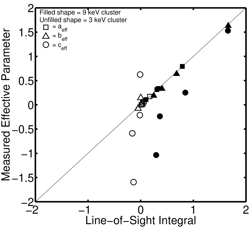
Figure 15: Best fit $\textbf{\emph{a}}_{\mathrm{eff}}$ from simulated, noise-free, ACT-like SZ images found using a Markov chain versus $\int\mathrm{C}d\textbf{\emph{p}}$ integrated along the cluster line of sight. The results for four different lines of sight through both the 9 keV and 3 keV simulated clusters are plotted. The lines of sight are 0’, 1’, 1.5’, and 2’ from the central pixel of the simulated SZ images. $d\textbf{\emph{p}}=(Td\tau,vd\tau,T^{2}d\tau)$, and $\mathrm{C}$ is a matrix of constants introduced in eq. (5). $\square$ = $a_{\mathrm{eff}}$, $\triangle$ = $b_{\mathrm{eff}}$, and $\bigcirc$ = $c_{\mathrm{eff}}$, and filled (unfilled) shapes correspond to the 9 keV (3 keV) cluster. Typical error bars for $1\mu K$ detector noise per 1’ beam are $\pm$ 0.04, $\pm$ 0.3, and $\pm$ 3 for $a_{\mathrm{eff}}$, $b_{\mathrm{eff}}$, and $c_{\mathrm{eff}}$ respectively.

Figure 15 shows this correspondence more explicitly. Plotted on the y-axis are best-fit $\textbf{\emph{a}}_{\mathrm{eff}}$ obtained via a MCMC using intensities from simulated noise-free SZ images of the 9 keV and 3 keV clusters assuming ACT-like observations. On the x-axis are plotted $\int\mathrm{C}d\textbf{\emph{p}}_{i}$ for the corresponding lines of sight. Four different lines of sight through both the 9 keV and 3 keV simulated clusters are plotted. These lines of sight are 0’, 1’, 1.5’, and 2’ from the central pixel of the simulated SZ images. Filled shapes correspond to the 9 keV cluster and unfilled shapes to the 3 keV cluster. For the $a_{\mathrm{eff}}$ and $b_{\mathrm{eff}}$ parameters, which can be well constrained, their equivalence to $\int\mathrm{C}d\textbf{\emph{p}}_{i}$ is extremely close. This confirms the near linearity of the SZ intensity shift with respect to the a, b, and c parameters. The $c_{\mathrm{eff}}$ parameters demonstrate some scatter around the $y=x$ line, and this is because the degeneracy in the $c$ direction prevents a MCMC from settling on the correct $c_{\mathrm{eff}}$ value.

If we could tightly constrain $a_{\mathrm{eff}}$, $b_{\mathrm{eff}}$, and $c_{\mathrm{eff}}$ via SZ measurements, we could solve for the quantities $\tau T_{\tau}$, $\tau v_{\tau}$, and $\tau(T^{2})_{\tau}$, where the subscript $\tau$ corresponds to optical-depth-weighted integrals (e.g. $T_{\tau}=\int Td\tau/\int d\tau$). From these one can find $T_{y}$, $\tau T_{\tau}/T_{y}$, and $v_{\tau}T_{y}/T_{\tau}$, following the algebra in Knox et al. (2004), where the subscript $y$ corresponds to a pressure-weighted integral. Therefore SZ measurements would constrain the pressure-weighted temperature (arising from the relativistic corrections), the optical-depth-weighted velocity times a correction factor and the optical depth times a similar correction factor which is the ratio of different weighted temperatures. Since degeneracies will allow SZ measurements to constrain only $a_{\mathrm{eff}}$ and $b_{\mathrm{eff}}$, information from an external source will be needed to constrain the above physically interesting quantities.

7 BREAKING PARAMETER DEGENERACY WITH AN X-RAY MEASUREMENT OF $T_{e}$

7.1 Measured Effective Velocity is approximately $\int vd\tau/\int d\tau$

Assuming contamination sources can be dealt with effectively, future SZ observations should be able to constrain two quantities given by

$$a_{\mathrm{eff}} \approx \tau(c_{1}T_{\tau}+c_{2}(T^{2})_{\tau})+c_{3}\tau v_{\tau}{\textrm{\hskip 8.5359pt and}}$$ (6)

$$b_{\mathrm{eff}} \approx \tau(c_{4}T_{\tau}+c_{5}(T^{2})_{\tau})+c_{6}\tau v_{\tau},$$ (7)

where the $c$’s are elements of the matrix $\mathrm{C}$ defined in eq. (5). It is conceivable that temperature measurements from an X-ray survey of clusters could allow the determination of $\tau$ and $v_{\tau}$.

Formally X-ray observations would need to provide a constraint on $c_{i}T_{\tau}+c_{j}(T^{2})_{\tau}$, where the $c$’s are known constants. However, $T_{\tau}$ and $(T^{2})_{\tau}$ are not obviously given by X-ray observations. An X-ray derived temperature is also not equivalent to $T_{\tau}$. The two may differ by as much as 1 keV (Mathiesen & Evrard, 2001). If X-ray observations gave $T_{x}=T_{\tau}$ and it was true that $(T_{\tau})^{2}=(T^{2})_{\tau}$, then the effective velocity we would get from a MCMC, after adding the $T_{x}$ prior, would be equal to $v_{\tau}$. For our 9 keV simulated cluster, $(T_{\tau})^{2}$ and $(T^{2})_{\tau}$ agree to within $5\%$ on average, and for our 3 keV simulated cluster, the two agree to within $12\%$ on average.

To get an estimate of the biases incurred by not having the correct weighted temperatures, we assume $(T_{\tau})^{2}=(T^{2})_{\tau}$ and add a temperature prior of $T_{\tau}$ to our MCMC. Adding a $T_{\tau}$ prior, in the manner we discuss further in §7.2, we find for the central pixel of the 9 keV cluster, from simulated, noise-free, ACT-like SZ images, an effective velocity of 230 km/sec from the MCMC and an optical-depth-weighted line-of-sight velocity of 218 km/sec from the three dimensional cluster simulation. For the central pixel of the 3 keV cluster SZ image, we find an effective velocity of -10 km/sec from the MCMC and an optical-depth-weighted line-of-sight velocity of -3 km/sec from the three dimensional cluster simulation. The bias between the velocity from the MCMC and $v_{\tau}$ is most likely due to the breakdown of the $(T_{\tau})^{2}=(T^{2})_{\tau}$ assumption.

To quantify the bias incurred from $T_{x}$ differing from $T_{\tau}$, we add a $\pm$ 1 keV offset to our $T_{\tau}$ prior. We find for the central pixel of the 9 keV cluster SZ image, an effective velocity of 228 km/sec from the MCMC for both + and - 1 keV offsets. We find for the central pixel of the 3 keV cluster SZ image, an effective velocity of -45 km/sec from the MCMC for a + 1keV offset and an effective velocity of 6 km/sec for a - 1 keV offset. This would suggest a total bias between the measured effective velocity and $v_{\tau}$ of about 15 km/sec for the 9 keV cluster and between 10 and 40 km/sec for the 3 keV cluster.

7.2 MCMC Errors on $v_{\mathrm{eff}}$ and $\tau$ Given an X-ray $T_{\mathrm{eff}}$ Prior

To determine realistic errors on $v_{\mathrm{eff}}$ and $\tau$ from adding a measurement of $T_{\mathrm{eff}}$ to our simulated SZ data, we again use a MCMC. We weight each point in our MCMC by the factor $e^{-((T-T_{\mathrm{eff}})/\Delta T_{\mathrm{eff}})^{2}/2}$ where we calculate $T_{\mathrm{eff}}=\int T_{e}d\tau/\int d\tau$ from the 3D cluster simulation and $\Delta T_{\mathrm{eff}}$ is the assigned measurement error on $T_{\mathrm{eff}}$.

For a 1 keV error on $T_{\mathrm{eff}}$, our ACT simulation of the 9 keV cluster gives $\sigma_{v}=20$ km/sec and $\sigma_{\tau}=0.002$ for the central pixel. Our ACT simulation of the 3 keV cluster gives $\sigma_{v}=60$ km/sec and $\sigma_{\tau}=0.004$ for the central pixel. Assuming a 2 keV error on $T_{\mathrm{eff}}$, the ACT simulation of the 9 keV cluster gives $\sigma_{v}=40$ km/sec and $\sigma_{\tau}=0.004$, and the ACT simulation of the 3 keV cluster gives $\sigma_{v}=100$ km/sec and $\sigma_{\tau}=0.005$. Our Planck simulation of the 9 keV cluster gives $\sigma_{v}=500$ km/sec and $\sigma_{\tau}=0.0024$ for a 1 keV error on $T_{\mathrm{eff}}$ and $\sigma_{v}=560$ km/sec and $\sigma_{\tau}=0.0062$ for a 2 keV error, for the central pixel. Table 2 lists these 1-$\sigma$ errors for convenient reference.

The errors obtained on $\sigma_{v}$ and $\sigma_{\tau}$ from our MCMC are smaller than those obtained using a Fisher matrix. However, the MCMC errors are more accurate than those from a Fisher matrix since a Fisher matrix approximates the likelihood surface by an ellipsoidal Gaussian, which can result in overestimated errors for likelihood surfaces with strong spatial curvature such as these. These results show that, in the absence of contamination from imperfect point source and primary microwave background removal, adding X-ray temperature measurements to the data from upcoming ACT-like SZ surveys can determine cluster peculiar velocities to within 100 km/sec or less. Large-scale velocity fields obtained from galaxy clusters out to high redshift could provide an interesting probe of dark matter and dark energy.

8 SOURCES OF CONTAMINATION TO THE SZ SIGNAL

Major sources of possible contamination have been neglected in this exercise. In particular, it is possible that primary and secondary microwave fluctuations and point sources (both radio and infrared) could be problematic.

Primary fluctuations are in some ways both the largest and the smallest concern. The fluctuation amplitudes are on the order of 100 $\mu K$ and have the exact same spectral behavior as the kinematic SZ effect, providing a noise source that is an order of magnitude larger than the signal. However, these fluctuations will be highly coherent over the extent of the cluster, so the pixel-by-pixel component separation will naturally measure this extended emission. At that point, a simple spatial filter can be applied to remove the primary microwave fluctuations. This spatial filter will have the effect of removing roughly half of the cluster kinematic SZ signal (Holder, 2004), thereby reducing the signal-to-noise by approximately this same factor.

Secondary fluctuations will be dominated by kinematic SZ from the quasi-linear regime (the Vishniac effect; Vishniac (1987)) and the thermal SZ background. The kinematic SZ fluctuations are expected to be below the pixel noise, and therefore subdominant, the thermal SZ background will simply add noise to the component that is separated as thermal SZ. The rms is expected to be roughly 10 $\mu K$, which will most likely serve as the dominant source of noise for this component. However, this is much smaller than the expected thermal SZ signal from each cluster and should not impact the component separation process at a noticeable level.

Radio point sources that are uncorrelated with galaxy clusters are not a concern (Knox et al., 2004), but radio point sources within galaxy clusters can “fill in” the SZ decrement and severely impact cluster SZ measurements. This is a long-standing concern for low frequency SZ measurements (Moffett & Birkinshaw, 1989), and could be a concern even at frequencies as high as 150 GHz. The spectra of radio sources up to such high frequencies are not well known, but very rough estimates can be made of the most likely contamination. Radio surveys at 1.4 GHz have been done of nearby Abell clusters (Ledlow & Owen, 1996) and distant X-ray selected clusters (Stocke, 1999) that find that a typical galaxy cluster has of order one radio source at 1.4 GHz that would be of order a few mJy at a cosmological distance. Detailed studies of spectra of bright radio sources indicate (Herbig & Readhead, 1992) that typical radio sources have spectra that are falling and steepening with frequency. In particular, in their sample they found only a handful of sources that were as bright at 40 GHz as at 1.4 GHz. Most sources with rising spectra at 1.4 GHz eventually turned over and had lower fluxes at 40 GHz than at 1.4 GHz, indicating that studies based on spectral indices at low frequency will not provide accurate estimates of behavior at high frequencies. Assuming that cluster sources have the same spectral behavior and that the steepening at high frequencies continues, this would indicate that only a few percent of clusters will have a radio source contributing of order mJy flux at 150 GHz. In this handful of clusters, radio sources will be a concern, as this flux would be an order of magnitude larger than the pixel noise. However, in the majority of clusters the contamination due to cluster radio galaxies would be comparable to or smaller than the pixel noise.

Infrared point sources, consisting largely of dusty star forming galaxies, are likely to be a major source of contamination (Knox et al., 2004; White & Majumdar, 2004). A detailed treatment is beyond the scope of this paper, but the results of Knox et al. (2004) suggest that hot clusters (with temperatures above about 6 keV) will have a large enough SZ signal that the infrared point sources can be estimated simultaneously with the thermal SZ and kinematic SZ signals, assuming an independent measure of the gas temperature. In this work we have found that the three measurements by an ACT-like experiment provide only two effective constraints, suggesting that there is redundancy in the measurements and that an additional degree of freedom (infrared point sources) could be allowed without significantly degrading the constraints. The surest solution is to use ALMA to measure the relevant point source fluxes. As a point of comparison, ALMA could image 100 square degrees (comparable to the ACT survey area) to a point source sensitivity of 0.1 mJy at 140 GHz in less than 1 month. If one were to instead focus on the inner 2’ of the largest 100 galaxy clusters, this would take several hours of observing time. Note that these same observations could be used to estimate the SZ effects, but the small primary beam of ALMA (due to the large telescopes) would require careful mosaicing of the cluster to avoid resolving out much of the cluster flux.

9 DISCUSSION AND CONCLUSIONS

Instruments such as ACT, SPT, APEX, and Planck will find thousands of galaxy clusters in the near future via SZ observations. In addition to determining the number density of clusters, which can put limits on cosmological parameters, these surveys will reveal information about the gas properties of individual clusters. Ideally, SZ observations would be made in at least three frequency bands with one frequency around 300 GHz, one around 150 GHz, and another either near 90 GHz or better yet near 30 GHz. Arcminute-resolution observations at those frequencies with $\simeq 1\mu K$ detector noise would tightly constrain the cluster gas temperature, line-of-sight velocity, and optical depth in the absence of excessive point source and primary microwave background contamination from imperfect subtraction. Without this set of SZ observations, parameter degeneracies prevent disentanglement of these three cluster parameters.

Current limitations in technology and instrument availability will make it impractical to obtain 30 GHz, arcminute-resolution, $1\mu K$ sensitivity, SZ observations of the majority of the clusters that will be found. SZ surveys that will have 90 GHz channels will still have parameter degeneracies resulting from detector noise $\simeq 10\mu K$. However, we find that upcoming SZ surveys will be able to tightly constrain two cluster gas parameters which are linear combinations of $\tau T_{e}$, $\tau v$, and $\tau T_{e}^{2}$. The constrained parameters are roughly $\tau T_{e}$ and a single linear combination of the other two terms. We demonstrated that this is the case for both individual isothermal gas regions and for 3D simulated Nbody + hydro clusters.

The SZ intensity shift that microwave photons experience passing through a cluster is nearly a linear function of $\tau T_{e}$, $\tau v$, and $\tau T_{e}^{2}$, these being the most dominant terms in the intensity shift expression. This near-linearity results in a close correspondence between the two effective parameters SZ surveys will constrain and simple line-of-sight integrals of these parameters through the three dimensional cluster. We illustrated this correspondence with our three dimensional cluster simulations. This will greatly simplify data analysis of multi-frequency SZ data: it will not be necessary (or useful) to model the intensity as a superposition of elements along the line of sight but instead the SZ effect can be modeled as a single gas element with a single effective temperature and velocity.

We have shown that a temperature constraint added to SZ data breaks the parameter degeneracy between $\tau$, $T_{\mathrm{eff}}$, and $v_{\mathrm{eff}}$. Using the above linearity, we show that the effective velocity constrained by combining SZ with an independent temperature measure is approximately the optical-depth-weighted velocity integrated along the cluster line of sight. Since X-ray derived temperatures do not give us precisely the weighted temperature measurements that are required to determine $\int vd\tau/\int d\tau$ exactly, we find the measured effective velocity will be biased away from $\int vd\tau/\int d\tau$ by about 15 to 40 km/sec, with a smaller bias for hotter, relaxed clusters.

Errors on $\tau$ and $v_{\mathrm{eff}}$ are calculated via a Markov chain Monte Carlo method assuming a temperature prior in addition to SZ data. We find for ACT-like SZ simulations of our 9 keV cluster, $\sigma_{v}$ = 20 km/sec and $\sigma_{\tau}$ = 0.002 for a 1 keV error on $T_{\mathrm{eff}}$, and $\sigma_{v}$ = 40 km/sec and $\sigma_{\tau}$ = 0.004 for a 2 keV error on $T_{\mathrm{eff}}$. For our 3 keV simulated cluster, $\sigma_{v}$ = 60 km/sec and $\sigma_{\tau}$ = 0.004, and $\sigma_{v}$ = 100 km/sec and $\sigma_{\tau}$ = 0.005 for 1 keV and 2 keV errors on $T_{\mathrm{eff}}$ respectively. The Markov chain errors we find on $v_{\mathrm{eff}}$ and $\tau$ are smaller than those obtained via a Fisher matrix. A Fisher matrix overestimates the errors because the likelihood surface is strongly curved in this parameter representation, strongly violating the implicit assumption of ellipsoidal symmetry over the parameter region of interest. Note that the errors on velocities will be increased when residual primary microwave contamination is included, and that bulk flows within the clusters provide comparable noise in matching observed peculiar velocities to the true bulk velocity of the cluster (Nagai et al., 2003; Holder, 2004; Diaferio et al., 2005).

If an independent cluster temperature estimate from X-ray spectroscopy is unavailable, temperature estimates can also be obtained from either the cluster velocity dispersion (Lubin & Bahcall, 1993) or the cluster integrated SZ flux (Benson et al., 2004) and scaling relations. Since an accuracy of only 2 keV is required on an additional temperature measurement to obtain very interesting velocity estimates, the use of these scaling relations could prove to be a very beneficial tool.

As discussed in §8, contamination from primary microwave background fluctuations and point sources add another source of noise that must be factored into these parameter constraints. Radio point sources due to emission from galaxy cluster members themselves and infrared point sources will both be non-negligible sources of SZ signal contamination. Studies of the effect point source contamination will have on cluster parameter extraction have been carried out by Knox et al. (2004) and Aghanim et al. (2004). Both studies have found that the contamination could potentially be serious; however the latter study considers the effect of point source contamination if no attempt is made to filter point sources out of the observations or model them into the parameter extraction routines. Moreover, even in the worst case point source contamination scenario, observations with an instrument such as ALMA will allow straightforward point source subtraction from SZ images. Clearly either filtering techniques or additional ALMA type observations will be needed to minimize both the point source and primary microwave background contamination of SZ signals.

Near-future SZ surveys will open the door to a wealth of information about galaxy clusters. Determining the number density of galaxy clusters as a function of redshift is potentially a strong probe of dark energy’s equation of state and variability over time (Haiman et al., 2001; Holder et al., 2001; Hu, 2003; Majumdar & Mohr, 2003, 2004). However, galaxy clusters offer more information that can also yield cosmological information. The kinematic SZ signature of galaxy clusters can reveal large-scale velocity fields out to high redshift that can provide an alternative probe of large-scale dark matter and dark energy (Peel & Knox, 2003). Cluster optical depth information yields cluster gas mass estimates, and optical depths are crucial to any of the tests that have been proposed using the (extremely difficult to measure) polarization of scattered microwave photons at the position of galaxy clusters (Kamionkowski & Loeb, 1997). The gas parameters $T_{e}$, $\tau$, and $v$ of individual galaxy clusters are of direct interest for cluster astrophysics. Arcminute-resolution SZ observations can begin to probe cluster substructure and offer more information about cluster gas profiles and internal gas dynamics. In summary, SZ observations are entering new territory, where large scale surveys will offer new understandings of galaxy clusters and cosmology.

Observing	Detector	$kT_{e}$	$v$	$\tau$	$\sigma_{T_{e}}$	$\sigma_{v}$
Frequencies (GHz)	Noise ($1\mu K$)	(keV)	(km/sec)		(keV)	(km/sec)
30, 150, 300	1	10	200	0.012	0.5	25
90, 150, 300	1	10	200	0.012	1	50
145, 225, 265	1	10	200	0.012	6	220
30, 150, 300	1	10	-200	0.012	0.5	50
90, 150, 300	1	10	-200	0.012	1	100
145, 225, 265	1	10	-200	0.012	6.5	400
30, 145, 225, 265	1	10	200	0.012	0.5	25
90, 145, 225, 265	1	10	200	0.012	1	50
30, 150, 300	10	10	200	0.012	5	200
90, 150, 300	10	10	200	0.012	8	250
145, 225, 265	10	10	200	0.012	9	350
30, 150, 300	1	7	200	0.009	1	50
30, 150, 300	1	3	200	0.004	3.5	200

Table 1: The 1-$\sigma$ errors on $T_{e}$ and $v$ for different observing frequencies, detector noise, and gas parameters.

Simulated	Simulated Cluster	Error on Temp.	$\sigma_{\tau}$	$\sigma_{v}$
Experiment	Avg. Temp. (keV)	Prior (keV)		(km/sec)
ACT-like	9	1	0.002	20
ACT-like	3	1	0.004	60
ACT-like	9	2	0.004	40
ACT-like	3	2	0.005	100
Planck-like	9	1	0.002	500
Planck-like	9	2	0.006	560

Table 2: The 1-$\sigma$ errors on $\tau$ and $v$ for ACT-like and Planck-like experiments using 9 keV and 3 keV simulated clusters with varying errors on the temperature prior $T_{\mathrm{eff}}$.

$\begin{array}[]{c@{\hspace{0.1in}}c@{\hspace{0.1in}}c}\includegraphics[width=433.62pt]{f1a.eps}\hfil\hskip 7.22743pt&\includegraphics[width=433.62pt]{f1b.eps}\hfil\hskip 7.22743pt&\includegraphics[width=433.62pt]{f1c.eps}\cr\mbox{\hskip 18.7898pt(a)}\hfil\hskip 7.22743pt&\mbox{\hskip 18.7898pt(b)}\hfil\hskip 7.22743pt&\mbox{\hskip 18.7898pt(c)}\end{array}$

Figure 1: 1-$\sigma$ likelihood contours for a simulated region of gas of $T_{e}$ = 10 keV ($1.2\times 10^{8}$ K), $v$ = 200 km/sec, and $\tau$ = 0.012 obtained by calculating the SZ effect for three different observing frequency sets assuming $1\mu K$ detector noise. The frequency sets are 1a) 30, 150, 300 GHz, 1b) 90, 150, 300 GHz, and 1c) 145, 225, 265 GHz. The SZ intensity shifts from the gas region are calculated using the formula in Nozawa et al. (1998), and the ratios of the intensity shifts at different frequencies in each set are computed to eliminate the dependence on optical depth. A dot ($\bullet$) marks the input fiducial gas region.

$\begin{array}[]{c@{\hspace{0.1in}}c@{\hspace{0.1in}}c}\includegraphics[width=433.62pt]{f2a.eps}\hfil\hskip 7.22743pt&\includegraphics[width=433.62pt]{f2b.eps}\hfil\hskip 7.22743pt&\includegraphics[width=433.62pt]{f2c.eps}\cr\mbox{\hskip 18.7898pt(a)}\hfil\hskip 7.22743pt&\mbox{\hskip 18.7898pt(b)}\hfil\hskip 7.22743pt&\mbox{\hskip 18.7898pt(c)}\end{array}$

Figure 2: Same as Fig. 1 except for $v$ = -200 km/sec.

$\begin{array}[]{c@{\hspace{0.1in}}c@{\hspace{0.1in}}c}\includegraphics[width=433.62pt]{f3a.eps}\hfil\hskip 7.22743pt&\includegraphics[width=433.62pt]{f3b.eps}\hfil\hskip 7.22743pt&\includegraphics[width=433.62pt]{f3c.eps}\cr\mbox{\hskip 18.7898pt(a)}\hfil\hskip 7.22743pt&\mbox{\hskip 18.7898pt(b)}\hfil\hskip 7.22743pt&\mbox{\hskip 18.7898pt(c)}\end{array}$

Figure 3: Same as Fig. 1 except for detector noise of $10\mu K$.

$\begin{array}[]{c@{\hspace{0.1in}}c}\includegraphics[width=433.62pt]{f4a.eps}\hfil\hskip 7.22743pt&\includegraphics[width=433.62pt]{f4b.eps}\cr\mbox{\hskip 18.7898pt(a)}\hfil\hskip 7.22743pt&\mbox{\hskip 18.7898pt(b)}\end{array}$

Figure 4: Same as Fig. 1a except for gas $T_{e}$ and $\tau$ values: 4a) $T_{e}$ = 7 keV, $\tau$ = 0.009; 4b) $T_{e}$ = 3 keV, $\tau$ = 0.004.

$\begin{array}[]{c@{\hspace{0.11in}}c@{\hspace{0.11in}}c}\includegraphics[width=433.62pt]{f5a.eps}\hfil\hskip 7.94974pt&\includegraphics[width=433.62pt]{f5b.eps}\hfil\hskip 7.94974pt&\includegraphics[width=433.62pt]{f5c.eps}\cr\mbox{\hskip 18.7898pt(a)}\hfil\hskip 7.94974pt&\mbox{\hskip 18.7898pt(b)}\hfil\hskip 7.94974pt&\mbox{\hskip 18.7898pt(c)}\end{array}$

Figure 5: Projected 1-$\sigma$ likelihood contours for the ($T_{e}$, $v$, $\tau$) parameter space from SZ intensity shifts at 145, 225, and 265 GHz for a simulated gas region of $T_{e}$ = 10 keV ($1.2\times 10^{8}$ K), $v$ = 200 km/sec, and $\tau$ = 0.012 assuming $1\mu K$ detector noise.

$\begin{array}[]{c@{\hspace{0.1in}}c@{\hspace{0.1in}}c}\includegraphics[width=433.62pt]{f6a.eps}\hfil\hskip 7.22743pt&\includegraphics[width=433.62pt]{f6b.eps}\hfil\hskip 7.22743pt&\includegraphics[width=433.62pt]{f6c.eps}\cr\mbox{\hskip 18.7898pt(a)}\hfil\hskip 7.22743pt&\mbox{\hskip 18.7898pt(b)}\hfil\hskip 7.22743pt&\mbox{\hskip 18.7898pt(c)}\end{array}$

Figure 6: Same as Fig. 5 except for the parameter space ($\tau T_{e}$, $\tau v$, $\tau T_{e}^{2}$), corresponding to the physical parameters expected to be important.

$\begin{array}[]{c@{\hspace{0.1in}}c@{\hspace{0.1in}}c}\includegraphics[width=433.62pt]{f7a.eps}\hfil\hskip 7.22743pt&\includegraphics[width=433.62pt]{f7b.eps}\hfil\hskip 7.22743pt&\includegraphics[width=433.62pt]{f7c.eps}\cr\mbox{\hskip 10.84006pt(a)}\hfil\hskip 7.22743pt&\mbox{\hskip 10.84006pt(b)}\hfil\hskip 7.22743pt&\mbox{\hskip 10.84006pt(c)}\end{array}$

Figure 7: Same as Fig. 5 except for the parameter space ($a$, $b$, $c$), the combinations of the physical parameters that are best constrained by SZ observations.

$\begin{array}[]{c@{\hspace{0.005in}}c@{\hspace{0.005in}}c@{\hspace{0.005in}}c}\includegraphics[width=433.62pt]{f8a.eps}\hfil\hskip 0.3617pt&\includegraphics[width=433.62pt]{f8b.eps}\hfil\hskip 0.3617pt&\includegraphics[width=433.62pt]{f8c.eps}\hfil\hskip 0.3617pt&\includegraphics[width=433.62pt]{f8d.eps}\cr\mbox{}\hfil\hskip 0.3617pt&\mbox{(a)}\hfil\hskip 0.3617pt&\mbox{(b)}\hfil\hskip 0.3617pt&\mbox{(c)}\end{array}$

Figure 8: SZ simulations of a simulated Nbody+hydro cluster before smoothing and adding detector noise. The cluster is about $10^{15}M_{\odot}$, has an average gas temperature of about 9 keV, and is at z=0.43. Figures 8a, 8b, and 8c are of the 145, 225, and 265 GHz bands respectively. Each figure is about 6’ x 6’ with a pixel size of 0.02’ x 0.02’. The images are converted to temperature differences from the mean microwave background temperature. The color scale is from -100$\mu K$ to 100$\mu K$. Primary microwave background fluctuations and point source contamination are not included.

$\begin{array}[]{c@{\hspace{0.005in}}c@{\hspace{0.005in}}c@{\hspace{0.005in}}c}\includegraphics[width=433.62pt]{f9a.eps}\hfil\hskip 0.3617pt&\includegraphics[width=433.62pt]{f9b.eps}\hfil\hskip 0.3617pt&\includegraphics[width=433.62pt]{f9c.eps}\hfil\hskip 0.3617pt&\includegraphics[width=433.62pt]{f9d.eps}\cr\mbox{}\hfil\hskip 0.3617pt&\mbox{(a)}\hfil\hskip 0.3617pt&\mbox{(b)}\hfil\hskip 0.3617pt&\mbox{(c)}\end{array}$

Figure 9: Same as Fig. 8 except the cluster is about $2\times 10^{14}M_{\odot}$ and has an average gas temperature of about 3 keV.

$\begin{array}[]{c@{\hspace{0.005in}}c@{\hspace{0.005in}}c@{\hspace{0.005in}}c}\includegraphics[width=433.62pt]{f10a.eps}\hfil\hskip 0.3617pt&\includegraphics[width=433.62pt]{f10b.eps}\hfil\hskip 0.3617pt&\includegraphics[width=433.62pt]{f10c.eps}\hfil\hskip 0.3617pt&\includegraphics[width=433.62pt]{f10d.eps}\cr\mbox{}\hfil\hskip 0.3617pt&\mbox{(a)}\hfil\hskip 0.3617pt&\mbox{(b)}\hfil\hskip 0.3617pt&\mbox{(c)}\end{array}$

Figure 10: ACT-like SZ simulations of the 9 keV simulated cluster shown in Fig. 8 with 1’ resolution and $3\mu K$ gaussian random instrument noise in each 0.3’ x 0.3’ pixel. The remaining figure specifications are the same as in Fig. 8.

$\begin{array}[]{c@{\hspace{0.005in}}c@{\hspace{0.005in}}c@{\hspace{0.005in}}c}\includegraphics[width=433.62pt]{f11a.eps}\hfil\hskip 0.3617pt&\includegraphics[width=433.62pt]{f11b.eps}\hfil\hskip 0.3617pt&\includegraphics[width=433.62pt]{f11c.eps}\hfil\hskip 0.3617pt&\includegraphics[width=433.62pt]{f11d.eps}\cr\mbox{}\hfil\hskip 0.3617pt&\mbox{(a)}\hfil\hskip 0.3617pt&\mbox{(b)}\hfil\hskip 0.3617pt&\mbox{(c)}\end{array}$

Figure 11: Same as Fig. 10 except using the 3 keV simulated cluster shown in Fig. 9.

$\begin{array}[]{c@{\hspace{0.1in}}c@{\hspace{0.1in}}c}\includegraphics[width=433.62pt]{f12a.eps}\hfil\hskip 7.22743pt&\includegraphics[width=433.62pt]{f12b.eps}\hfil\hskip 7.22743pt&\includegraphics[width=433.62pt]{f12c.eps}\cr\mbox{\hskip 13.73148pt(a)}\hfil\hskip 7.22743pt&\mbox{\hskip 14.45377pt(b)}\hfil\hskip 7.22743pt&\mbox{\hskip 14.45377pt(c)}\end{array}$

Figure 12: The projected 1-$\sigma$ contours of the likelihood surface for the ($a_{\mathrm{eff}}$, $b_{\mathrm{eff}}$, $c_{\mathrm{eff}}$) parameter space from the central pixel of simulated ACT-like SZ images of a simulated 9 keV Nbody+hydro cluster. The likelihood contours are generated using a Markov chain and are for a given noise realization. The star ($\bigstar$) indicates the best fit $\textbf{\emph{a}}_{\mathrm{eff}}$ values from the Markov chain. The dot ($\bullet$) indicates the best fit $\textbf{\emph{a}}_{\mathrm{eff}}$ values obtained with an ideal instrument without detector noise. A diamond shape ($\blacklozenge$) marks the values of line-of-sight integrals through the three dimensional cluster.

$\begin{array}[]{c@{\hspace{0.1in}}c@{\hspace{0.1in}}c}\includegraphics[width=433.62pt]{f13a.eps}\hfil\hskip 7.22743pt&\includegraphics[width=433.62pt]{f13b.eps}\hfil\hskip 7.22743pt&\includegraphics[width=433.62pt]{f13c.eps}\cr\mbox{\hskip 14.45377pt(a)}\hfil\hskip 7.22743pt&\mbox{\hskip 15.89948pt(b)}\hfil\hskip 7.22743pt&\mbox{\hskip 16.62178pt(c)}\end{array}$

Figure 13: The projected 1-$\sigma$ contours of the likelihood surface for the ($a_{\mathrm{eff}}$, $b_{\mathrm{eff}}$, $c_{\mathrm{eff}}$) parameter space from the central pixel of simulated ACT-like SZ images of a simulated 3 keV Nbody+hydro cluster. The symbols within the contours are as for Fig. 12; note the axes are different scales.

$\begin{array}[]{c@{\hspace{0.1in}}c@{\hspace{0.1in}}c}\includegraphics[width=433.62pt]{f14a.eps}\hfil\hskip 7.22743pt&\includegraphics[width=433.62pt]{f14b.eps}\hfil\hskip 7.22743pt&\includegraphics[width=433.62pt]{f14c.eps}\cr\mbox{\hskip 14.45377pt(a)}\hfil\hskip 7.22743pt&\mbox{\hskip 15.17719pt(b)}\hfil\hskip 7.22743pt&\mbox{\hskip 15.17719pt(c)}\end{array}$

Figure 14: The projected 1-$\sigma$ contours of the likelihood surface for the ($a_{\mathrm{eff}}$, $b_{\mathrm{eff}}$, $c_{\mathrm{eff}}$) parameter space from the central pixel of simulated Planck-like SZ images of a simulated 9 keV Nbody+hydro cluster. The symbols within the contours are as for Fig. 12; note the axes are different scales.

References

- Aghanim et al. (2004) Aghanim, N., Hansen, S. H., Lagache, G. 2004, A&A, in press
- Aghanim et al. (2003) Aghanim, N., Hansen, S. H., Pastor, S., & Semikoz, D. V. 2003, JCAP, 5, 6
- Bennett et al. (2003) Bennett, C. L. et al. 2003, ApJS, 148, 97
- Benson et al. (2004) Benson, B. A., Ade, P. A. R., Bock, J. J., Ganga, K. M., Henson, C. N., Thompson, K. L., Church, S. E. 2004, AJ, 617, 829
- Birkinshaw (1999) Birkinshaw, M. 1999, Physics Reports, 310, 97
- Borys et al. (2003) Borys, C., Chapman, S., Halpern, M., & Scott, D. 2003, MNRAS, 344, 385
- Carlstrom et al. (2002) Carlstrom, J. E., Holder, G. P., & Reese, E. D. 2002, ARA&A, 40, 643
- Challinor & Lasenby (1998) Challinor, A., & Lasenby, A. 1998, ApJ, 499, 1.
- Christensen & Meyer (2001) Christensen, N., & Meyer, R. 2001, PhRvD, 64, 022001
- Christensen et al. (2001) Christensen, N., Meyer, R., Knox, L., & Luey, B. 2001, Classical Quant Grav, 18, 2677
- Diaferio et al. (2005) Diaferio, A. et al. 2005, MNRAS, 356, 1477
- Dodelson (2003) Dodelson, S. 2003, Modern Cosmology, San Diego, CA: Academic Press
- Dolgov et al. (2001) Dolgov, A. D., Hansen, S. H., Pastor, S., & Semikoz, D. V. 2001, ApJ, 554, 74
- Gilks et al. (1996) Gilks, W. R., Richardson, S., & Spiegelhalter, D. J.(Eds.), Markov Chain Monte Carlo in Practice, Boca Raton, FL: Chapman & Hall
- Haiman et al. (2001) Haiman, Z., Mohr, J. J., & Holder, G. P. 2001, ApJ, 553, 545
- Hansen (2004b) Hansen, S. H. 2004, MNRAS, 351, L5
- Hansen (2004a) Hansen, S. H. 2004, NewA, 9, 279
- Hansen et al. (2002) Hansen, S. H., Pastor, S., & Semikoz, D. V. 2002, ApJ, 573, L69
- Herbig & Readhead (1992) Herbig, T., & Readhead, A. C. S. 1992, ApJS, 81, 83
- Holder (2004) Holder, G. P. 2004, ApJ, 602, 18
- Holder et al. (2001) Holder, G. P., Haiman, Z., & Mohr, J. J. 2001, ApJ, 560, L111
- Hu (2003) Hu, W. 2004, PhRvD, 67, 081304
- Itoh et al. (1998) Itoh, N., Kohyama, Y., & Nozawa, S. 1998, ApJ, 502, 7
- Jackson (1991) Jackson, J. E. 1991, A User’s Guide to Principal Components, New York: John Wiley & Sons Inc.
- Kamionkowski & Loeb (1997) Kamionkowski, M., & Loeb, A. 1997, PhRvD, 56, 4511
- Kosowsky (2003) Kosowsky, A. 2003, NewAR, 47, 939
- Kosowsky et al. (2002) Kosowsky, A., Milosavljevic, M., & Jimenez, R. 2002, PhRvD, 66, 063007
- Knox et al. (2004) Knox, L., Holder, G. P., & Church, S. E. 2004, ApJ, 612, 96
- Kravtsov (1999) Kravtsov, A. V. 1999, Ph.D. Thesis
- Kravtsov et al. (2002) Kravtsov, A. V., Klypin, A., & Hoffman, Y. 2002, ApJ, 571, 563
- Ledlow & Owen (1996) Ledlow, M. J., & Owen, F. N. 1996, AJ, 112, 9
- Lewis & Bridle (2002) Lewis, A., & Bridle, S. 2002, PhRvD, 66, 103511
- Lubin & Bahcall (1993) Lubin, L. M., & , Bahcall N. A. 1993, ApJ, 415, L17
- Mathiesen & Evrard (2001) Mathiesen, B. F., & Evrard, A. E. 2001, ApJ, 546, 100
- Molnar & Birkinshaw (1999) Molnar, S. M., & Birkinshaw, M. 1999, ApJ, 523, 78
- Majumdar & Mohr (2004) Majumdar, S., & Mohr, J. J. 2004, ApJ, 613, 41
- Majumdar & Mohr (2003) Majumdar, S., & Mohr, J. J. 2003, ApJ, 585, 603
- Moffett & Birkinshaw (1989) Moffett, A. T., & Birkinshaw, M. 1989, AJ, 98, 1148
- Nagai et al. (2003) Nagai, D., Kravtsov, A. V., & Kosowsky A 2003, ApJ, 587, 524
- Nagai & Kravtsov (2003) Nagai, D., & Kravtsov, A. V. 2003, ApJ, 587, 514
- Nozawa et al. (1998) Nozawa, S., Itoh, N., & Kohyama, Y. 1998, ApJ, 508, 17
- Peel & Knox (2003) Peel, A., & Knox, L. 2003, Nuclear Phys B Proc Supp, 124, 83
- Pointecouteau et al. (1998) Pointecouteau, E., Giard, M., & Barret, D. 1998, A&A, 336, 44
- Press et al. (1997) Press, W. H, Teukolsky, S. A., Vetterling, W. T., & Flannery, B. P. 1997, Numerical Recipes in C, Second Edition, Cambridge, U. K.: Cambridge University Press
- Reese et al. (2002) Reese, E. D., Carlstrom, J. E., Joy, M., Mohr, J. J., Grego, L., Holzapfel, W. L. 2002, ApJ, 581, 53
- Rephaeli (1995) Rephaeli, Y. 1995, ARA&A, 33, 541
- Sazonov & Sunyaev (1998) Sazonov, S. Y., & Sunyaev, R. A. 1998, ApJ, 508, 1
- Sawicki & Webb (2004) Sawicki, M., & Webb, T. M. A. 2004, ApJ, in press
- Stocke (1999) Stocke, J. T. et al. 1999, AJ, 117, 1967
- Sunyaev & Zel’dovich (1970) Sunyaev, R. A., & Zel’dovich, Y. B. 1970, Comments Astrophys. Space Phys., 2, 66
- Sunyaev & Zel’dovich (1972) Sunyaev, R. A., & Zel’dovich, Y. B. 1972, Comments Astrophys. Space Phys., 4, 173
- Sunyaev & Zel’dovich (1980) Sunyaev, R. A., & Zel’dovich, Y. B. 1980, ARA& A, 18, 537
- Vishniac (1987) Vishniac, E. 1987, ApJ, 322, 597
- White & Majumdar (2004) White, M. & Majumdar, S. 2004, ApJ, 602, 565