Two-temperature accretion flows in magnetic cataclysmic variables: Structures of post-shock emission regions and X-ray spectroscopy

Abstract

We use a two-temperature hydrodynamical formulation to determine the temperature and density structures of the post-shock accretion flows in magnetic cataclysmic variables (mCVs) and calculate the corresponding X-ray spectra. The effects of two-temperature flows are significant for systems with a massive white dwarf and a strong white-dwarf magnetic field. Our calculations show that two-temperature flows predict harder keV spectra than one-temperature flows for the same white-dwarf mass and magnetic field. This result is insensitive to whether the electrons and ions have equal temperature at the shock but depends on the electron-ion exchange rate, relative to the rate of radiative loss along the flow. White-dwarf masses obtained by fitting the X-ray spectra of mCVs using hydrodynamic models including the two-temperature effects will be lower than those obtained using single-temperature models. The bias is more severe for systems with a massive white dwarf.

1 Introduction

Magnetic cataclysmic variables (mCVs) are close binaries containing a magnetic white dwarf accreting material from a Roche-lobe filling low-mass companion star (see e.g. Warner, 1995; Cropper, 1990). The material flow is supersonic when it leaves the inner Lagrangian point of the binary. It becomes subsonic near the white-dwarf surface, and a shock is formed, heating up the accreting material to temperatures $T\approx 3GM_{\rm w}m_{{}_{\rm H}}/8kR_{\rm w}\sim 10-50$ keV (where $G$ is the gravitational constant, $k$ the Boltzmann constant, $m_{{}_{\rm H}}$ the hydrogen-atomic mass, $M_{\rm w}$ the white-dwarf mass, and $R_{\rm w}$ the white-dwarf radius). The accreting material in the pre-shock flow is thereby photoionised. The post-shock flow is cooled by the emission of bremsstrahlung X-rays and cyclotron optical/IR radiation, as the material settles onto the white-dwarf atmosphere. The X-ray emission from a mCV depends on the temperature and density structures of the post-shock region, which in turn depends on the properties, mainly the temperature, of the accretion shock. As the shock temperature is determined by the mass and radius of the accreting white dwarf, we can infer the mass of the white dwarf from the X-ray spectra (Rothschild et al., 1981; Ishida et al., 1991; Wu et al., 1995; Fujimoto & Ishida, 1997; Ezuka & Ishida, 1999)

The X-ray spectra of mCVs, in particular the subclass intermediate polars (IPs), are well fitted by model spectra generated by the Aizu-type shock models (Aizu, 1973), such as those in Chevalier & Imamura (1982); Wu (1994); Wu et al. (1994) and Cropper et al. (1999). In these models, the electrons and ions have the same temperature locally (here termed a one-temperature model), but the temperature and density change along the flow in the post-shock region. It has been noticed that the white-dwarf masses obtained by the X-ray spectral fits using these models tend to be systematically larger than those derived from some other methods, e.g.  optical spectroscopy (see Ramsay et al., 1998; Ramsay, 2000).

The discrepancies could be due to inaccuracies in these other determinations. Alternatively, they may arise when the assumed absorption column density in fitting the X-ray data is uncertain. They could also be due to the fact that some relevant processes have not been considered in deriving the temperature and density structures of the post-shock emission region. In the one-temperature model, the electrons (the radiating particles) and the ions (the major energy-momentum carriers) are strongly thermally coupled and share the same temperatures. The coupling is maintained by electron-ion collisions. However, if the radiative cooling timescale of the accretion flow is shorter than the electron-ion collision timescale, the electrons will lose their energy rapidly while their energy gains via collisions are unable to keep up radiative loss. The two charged species then have unequal temperatures, and the accretion flow becomes a two-temperature flow. (See Wu, 2000; Beuermann, 2004, for recent reviews of accreting shocks in mCVs.)

Two-temperature flows are expected to occur in mCVs containing a white dwarf with a very strong magnetic field ($B~{}\ga~{}30$ MG): Lamb & Masters (1979) (see also Imamura, 1981; Imamura et al., 1987, 1996; Woelk & Beuermann, 1996; Saxton & Wu, 1999, 2001; Fischer & Beuermann, 2001). Cyclotron cooling is efficient in these systems, and two-temperature effects are most significant in the down-stream region just beneath the accretion shock. The electron temperature and density structures of a two-temperature accretion flow can be very different from those of a one-temperature flow. Moreover, the thicknesses of the high-density X-ray emitting region in the two flow models are expected to differ as well. Thus, the mass estimates obtained from a one-temperature post-shock model and a two-temperature post-shock model could be different.

Here we investigate the X-ray spectral properties of two-temperature accretion flows in mCVs. We consider a semi-analytical approch, in which the hydrodynamic models are constructed following the prescriptions of Imamura et al. (1987) and Saxton & Wu (2001). The thermal coupling between the ions and electrons is parametrised by the Coulomb collision rate. The radiative loss is due to the emission of bremsstrahlung X-rays, which is optically thin, and optical/IR cyclotron radiation, which could have substantial optical depths. The total radiative loss is approximated by a composite cooling function as in the previous studies of one-temperature flows by Wu (1994); Wu et al. (1994); Saxton (1999). We calculate the temperature and density structures of the two-temperature post-shock emission regions and generate the X-ray line and continuum spectra (§4) by convolving the MEKAL optically thin thermal plasmas model (Mewe et al., 1985; Kaastra & Mewe, 1993) in the XSPEC package. The results of the two-temperature calculations are compared with the results of one-temperature calculations (see e.g. Cropper et al., 1998; Tennant et al., 1998; Cropper et al., 1999).

2 Post-shock Accretion Flow: A Two-temperature Formulation

Our hydrodynamic formulation assumes that the gas in the post-shock region is completely ionised. The flow is along the magnetic field lines. We omit the gravitational force and the curvature of the field lines. These effects could be important when the thickness of post-shock region is significant in comparison with the white-dwarf radius. (See e.g. Cropper et al., 1999; Canalle et al., 2005.) Thus, the flow is perpendicular to the white-dwarf surface and is practically one-dimensional. Futhermore, we consider only the stationary situation. Hence, the hydrodynamic equations governing the flow are

$$v{{\partial\rho}\over{\partial x}}\ +\ \rho{{\partial v}\over{\partial x}} = 0\ ,$$ (1)

$${{\partial P_{\rm e}}\over{\partial x}}\ +\ {{\partial P_{\rm i}}\over{\partial x}}\ +\ \rho v{{\partial v}\over{\partial x}} = 0\ ,$$ (2)

$$v{{\partial P_{\rm e}}\over{\partial x}}\ -\ \gamma{{vP_{\rm e}}\over\rho}{{\partial\rho}\over{\partial x}} = (\gamma-1)~{}(\Gamma_{\rm ei}-\Lambda)\ ,$$ (3)

$$v{{\partial P_{\rm i}}\over{\partial x}}\ -\ \gamma{{vP_{\rm i}}\over\rho}{{\partial\rho}\over{\partial x}} = -(\gamma-1)~{}\Gamma_{\rm ei}\$$ (4)

where $v$ is the flow velocity, $\rho$ the density, $P_{\rm e}$ the electron partial pressure, $P_{\rm i}$ the ion partial pressure, $\Gamma_{\rm ei}$ the rate of the electron-ion energy exchange, $\Lambda$ the electron cooling function, and $\gamma$ the adiabatic index. The total gas pressure $P$ is the sum of the electron and ion partial pressures.

We assume an ideal gas law for both the electron and ion gases, i.e., $\gamma=5/3$ and $P_{\{\rm e,i\}}=n_{\{\rm e,i\}}~{}kT_{\{\rm e,i\}}$, where $n_{\rm e}$ is the electron number density, $n_{\rm i}$ the ion number density, $T_{\rm e}$ the electron temperature, and $T_{\rm i}$ the ion temperature. The rate of energy exchange due to electron-ion collision is $\Gamma_{\rm ei}\approx 3n_{\rm i}k(T_{\rm i}-T_{\rm e})/2t_{\rm ei}$, where $t_{\rm ei}$ is the equi-partition time, given by

$$t_{\rm ei}\ =\ {{3m_{\rm e}m_{\rm i}c^{3}}\over{8~{}(2\pi)^{1/2}Z_{i}^{2}n_{\rm e}e^{4}~{}{\rm ln}~{}C}}~{}\bigl{(}\theta_{\rm e}+\theta_{\rm i}\bigr{)}^{3/2}$$ (5)

(Spitzer, 1962), where $m_{\rm e}$ is the electron mass, $m_{\rm i}$ the ion mass, $c$ the speed of light, $e$ the electron charge, $\theta_{\rm e}=kT_{\rm e}/m_{\rm e}c^{2}$, $\theta_{\rm i}=kT_{\rm i}/m_{\rm i}c^{2}$, and ln $C$ the Coulomb logarithm. We have

$$\Gamma_{\rm ei}={{{4\sqrt{2\pi}e^{4}Z_{i}^{2}n_{\rm e}n_{\rm i}\ {\rm ln}~{}C}}\over{m_{\rm e}c}}~{}\bigg{\{}{{\theta_{\rm i}[1-(m_{\rm e}\theta_{\rm e}/m_{\rm i}\theta_{\rm i})]}\over{(\theta_{\rm e}+\theta_{\rm i})^{3/2}}}\bigg{\}}\ .$$ (6)

The composite cooling function $\Lambda$ consists of a bremsstrahlung cooling term $\Lambda_{\rm br}$ and a cyclotron cooling term $\Lambda_{\rm cy}$ (Wu et al., 1994), i.e.,

$$\Lambda \equiv \Lambda_{\rm br}+\Lambda_{\rm cy}$$ (7)

$$\approx \Lambda_{\rm br}~{}\bigg{[}~{}1+\epsilon_{\rm s}~{}\bigg{(}{T_{\rm e}\over T_{\rm e,s}}\bigg{)}^{2.0}\bigg{(}{n_{\rm e,s}\over n_{\rm e}}\bigg{)}^{1.85}\bigg{]}\ ,$$

where $\epsilon\equiv t_{\rm br}/t_{\rm cy}$ is the ratio of the bremsstrahlung-cooling timescale to the cyclotron-cooling timescale. (Here and elsewhere, the subscript $s$ denotes the value evaluated at the shock surface.) The derivation of the expression of $\epsilon_{\rm s}$ is given in Appendix A.3. The explicit form of the bremsstrahlung cooling function is

$$\Lambda_{\rm br}=16\bigg{(}{{2\pi}\over 3}\bigg{)}^{3/2}{e^{6}\over{m_{\rm e}c^{2}h}}\ Z_{i}^{2}n_{\rm e}n_{\rm i}\ \theta_{\rm e}^{1/2}\ g_{{}_{\rm B}}$$ (8)

(Rybicki & Lightman, 1979), where $h$ is the Planck constant and $g_{{}_{\rm B}}$ the Gaunt factor.

We note that our calculations depend on the functional form of $\Lambda_{\rm cy}$ in addition to the parameter $\epsilon_{\rm s}$. In (7) we have assumed a power-law type function to approximate the cyclotron radiative loss term. A key ingredient in constructing the cooling function is to estimate the frequency $\omega^{*}$ at which the local cyclotron spectrum peaks (see Wada et al., 1980; Saxton, 1999). How well the assumed power-law function approximates the cyclotron radiative loss depends on the accuracy of determining $\omega^{*}$ in a given geometrical and hydrodynamic setting. Here we follow the approach of Wada et al. (1980) and Saxton (1999), but the technique would be improved if we could construct a local cyclotron cooling function more self-consistently, say by using an iterative scheme that calculates the cyclotron emission spectrum of each stratum and uses it to readjust the local parameters of the cyclotron cooling function.

We ignore electron conduction, Compton scattering and nuclear burning in the energy transport. These processes are unimportant in the accretion flows of mCVs, unless the situation is very extreme, e.g.  the white dwarf is unusually massive ($\sim 1.2-1.4$ M_⊙) and the accretion rate is very high ($\dot{M}>0.1\dot{M}_{{}_{\rm E}}$, where $\dot{M}_{{}_{\rm E}}$ is the Eddington accretion rate) (Imamura et al., 1987). We do not include line cooling in our calculation of $\Lambda$. However, line cooling may not be negligible at the very bottom of the post-shock region where the temperature is low. For systems with low white-dwarf masses, the shock temperature and the post-shock gas temperature are low enough that the Fe L lines can actually contribute a significant fraction of the total cooling (see Mukai, 2003). A fully consistent treatment of line cooling in the hydrodynamic calculation is non-trivial, and we will leave this for future studies.

To simplify the hydrodynamic equations, we consider the dimensionless variables $\xi\equiv x/x_{\rm s}$, $\tau\equiv-v/v_{\rm ff}$, $\zeta\equiv\rho/\rho_{\rm a}$, $\pi_{\rm i}\equiv P_{\rm i}/\rho_{\rm a}v_{\rm ff}^{2}$, and $\pi_{\rm e}\equiv P_{\rm e}/\rho_{\rm a}v_{\rm ff}^{2}$, where $v_{{}_{\rm ff}}=(2GM_{\rm w}/R_{\rm w})^{1/2}$ is the free-fall velocity at the white-dwarf surface, $\rho_{\rm a}=\dot{m}/v_{\rm ff}$ the density of the pre-shock flow, and $\dot{m}$ the specific accretion rate. Substituting these variables into equations (1), (2), (3) and (4) yields

$$\tau{{\partial\zeta}\over{\partial\xi}}\ +\ \zeta{{\partial\tau}\over{\partial\xi}} = 0,$$ (9)

$${{\partial\pi_{\rm e}}\over{\partial\xi}}\ +\ {{\partial\pi_{\rm i}}\over{\partial\xi}}\ +\ \tau\zeta{{\partial\tau}\over{\partial\xi}} = 0,$$ (10)

$$\tau{{\partial\pi_{\rm e}}\over{\partial\xi}}\ -\ \gamma{{\tau\pi_{\rm e}}\over\zeta}{{\partial\zeta}\over{\partial\xi}} = {\tilde{\Lambda}}-{\tilde{\Gamma}}_{\rm ei}\ ,$$ (11)

$$\tau{{\partial\pi_{\rm i}}\over{\partial\xi}}\ -\ \gamma{{\tau\pi_{\rm i}}\over\zeta}{{\partial\zeta}\over{\partial\xi}} = {\tilde{\Gamma}}_{\rm ei}\ ,$$ (12)

where we define expressions for the non-dimensional energy exchange and cooling functions, ${\tilde{\Gamma}}_{\rm ei}=(\gamma-1)(x_{\rm s}/\rho_{\rm a}v_{\rm ff}^{3})~{}\Gamma_{\rm ei}$ and ${\tilde{\Lambda}}=(\gamma-1)(x_{\rm s}/\rho_{\rm a}v_{\rm ff}^{3})~{}\Lambda$.

The boundary values for electron and ion pressures ($\pi_{\rm e,s}$ and $\pi_{\rm i,s}$) are determined by the efficiency of the electron-ion coupling through the shock transition region. Their ratio, $\sigma{\rm{}_{s}}\equiv\pi_{\rm e,s}/\pi_{\rm i,s}$, can take values between $m_{\rm e}/m_{\rm i}$ (the ratio of the electron mass to the ion mass) and $\mu_{\rm i}/\mu_{\rm e}$ (the ratio of the molecular weight of the ions to that of the electrons), depending on the assumed coupling processes (Imamura et al., 1996). The physics of how the electrons couple with the ions at the shock is not well understood. The value of $\sigma_{\rm s}$ is really a dependent property of the pre-shock flow, but its derivation would require solving a comprehensive model of pre- and post-shock regions, with explicit radiative transfer and hydrodynamics: a complex task beyond the scope of the present work. We therefore treat $\sigma{\rm{}_{s}}$ as a free parameter and consider a few sensible values in our calculations to see what difference it will make to the density and temperature structures of the flows and the associated X-ray spectral properties.

For the other boundary conditions, we assume a strong-shock condition: at the shock surface ($\xi=1$), $\tau_{\rm s}=1/4$, $\zeta_{\rm s}=4$ and for the (unitless) total gas pressure ($\pi_{0}\equiv\pi{\rm{}_{e}}+\pi{\rm{}_{i}}$) we have $\pi_{\rm 0,s}=3/4$. At the bottom of the flow, we consider a “stationary wall” condition: $\tau=0$ at the white-dwarf surface ($\xi=0$). We omit the transfer of energy from beneath the white-dwarf atmosphere (see Wu & Cropper, 2001)

3 Temperature and Density Structures of the Post-shock Region

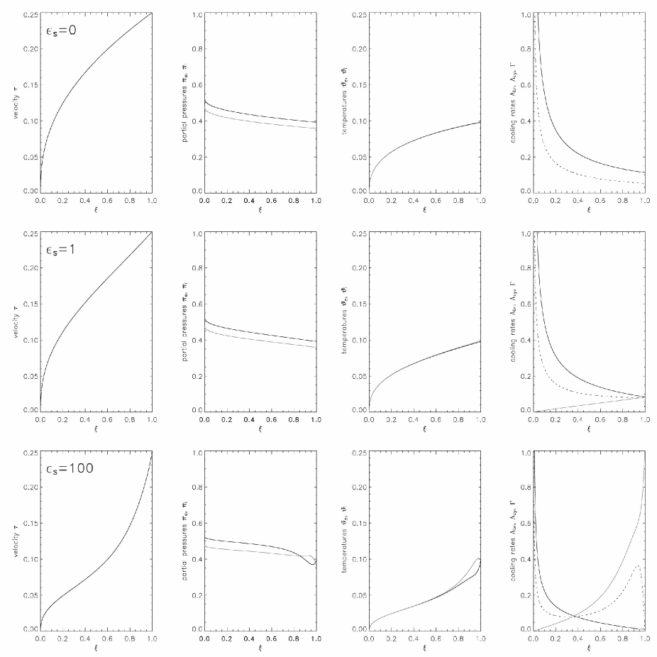
Figure 1: Stationary structures of accretion shocks with $(\sigma{\rm{}_{s}},\psi_{\rm ei})=(\overline{Z},10)$ and solar metallicity ($\overline{Z}={\overline{Z}}_{\odot}$). The parameter that sets the relative efficiency of cycloton cooling to bremsstrahlung cooling is $\epsilon{\rm{}_{s}}=0,1,100$, from top to bottom. The first column shows the flow velocity $\tau$. The second column shows the electron pressure $\pi{\rm{}_{e}}$ (black) and the ion pressure $\pi{\rm{}_{i}}$ (grey). The third column shows the electron temperature $\vartheta{\rm{}_{e}}\equiv\tau\pi{\rm{}_{e}}$ (black) and the ion temperature $\vartheta{\rm{}_{i}}\equiv\overline{Z}\tau\pi{\rm{}_{i}}$ (grey). The fourth column shows the local values of the normalised bremsstrahlung cooling rate (black), the normalised cyclotron cooling rate (grey), and the electron-ion exchange rate (dotted). These flows are quasi-one-temperature, and the two-temperature case with small $\epsilon{\rm{}_{s}}$ are practically indistinguishable from the one-temperature flows.

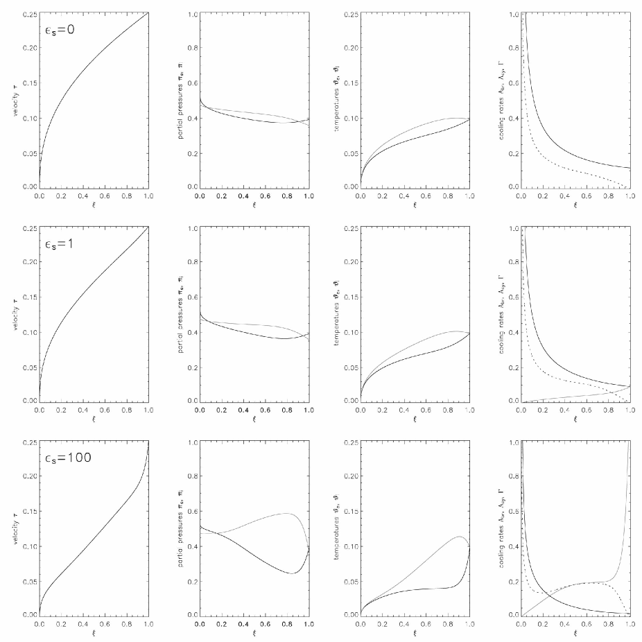
Figure 2: Stationary structures of two-temperature accretion shock. The system parameters are the same as those in Figure 1 except $(\sigma{\rm{}_{s}},\psi_{\rm ei})=(\overline{Z},0.2)$, i.e. the electron-ion collisional coupling are weaker.

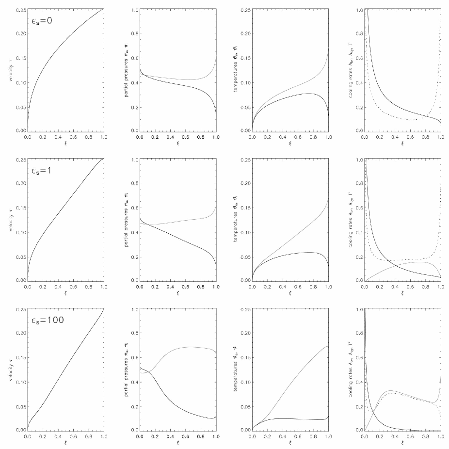
Figure 3: Stationary structures of two-temperature accretion shock. The system parameters are the same as those in Figures 1 and 2 except $(\sigma{\rm{}_{s}},\psi_{\rm ei})=(0.2,0.2)$.

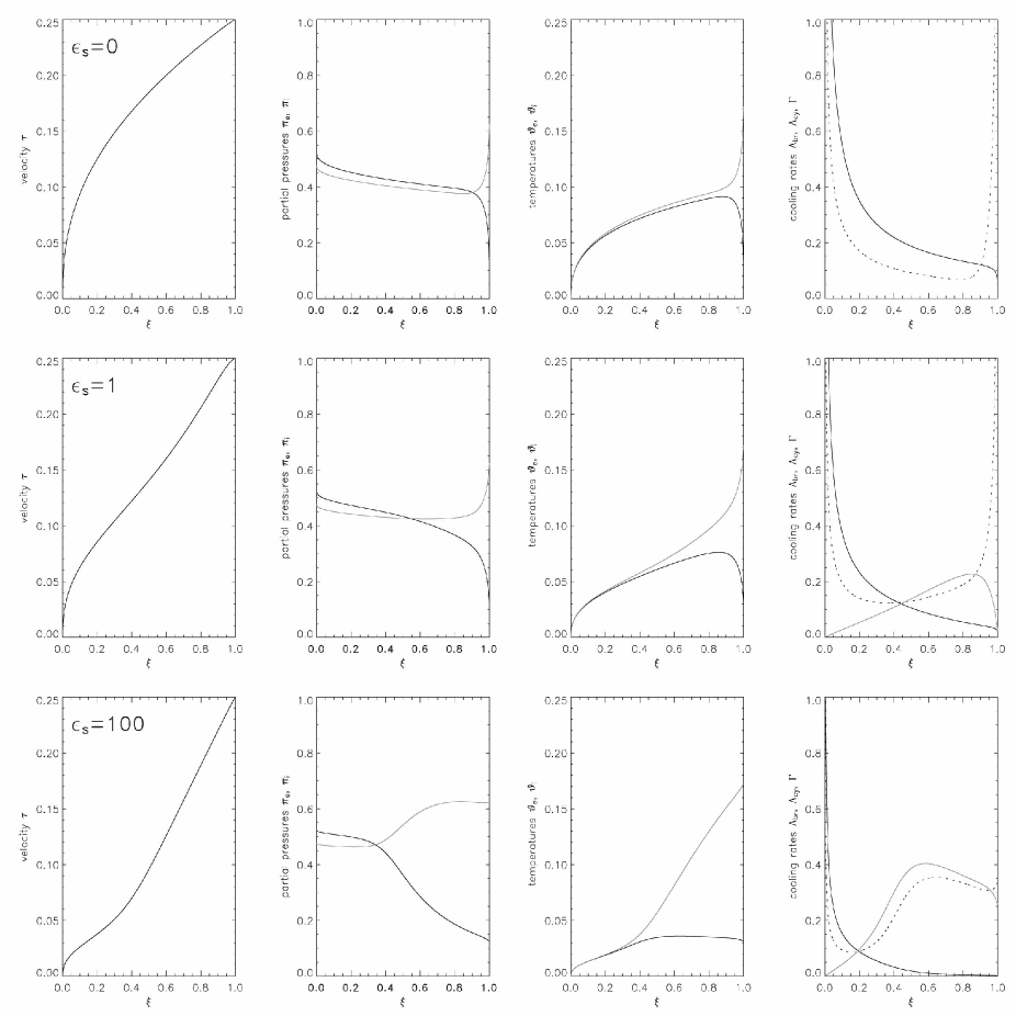
Figure 4: Stationary structures of two-temperature accretion shock. The system parameters are the same as those in Figures 1 and 2 except $(\sigma{\rm{}_{s}},\psi_{\rm ei})=(0.2,1)$.

We integrate the mass continuity and the momentum equations, yielding

$$\tau\zeta = 1,$$ (13)

$$\pi_{\rm 0} = 1-\tau.$$ (14)

Substituting these into the energy equations and eliminating $\pi_{\rm i}$, we obtain two differential equations:

$${{\partial\tau}\over{\partial\xi}}={{\tilde{\Lambda}}\over{\gamma(1-\tau)-\tau}}\ ;$$ (15)

$${{\partial\pi_{\rm e}}\over{\partial\xi}}={1\over\tau}\left[{\tilde{\Lambda}-{{\gamma\tau\pi_{\rm e}\tilde{\Lambda}}\over{\gamma(1-\tau)-\tau}}-\tilde{\Gamma}}\right]\ ,$$ (16)

where

$$\tilde{\Lambda}=(\gamma-1)x_{\rm s}\rho v_{\mathrm{ff}}^{-2}A\sqrt{{\pi_{\rm e}}\over{\tau^{3}}}[1+\epsilon_{\rm s}f(\tau,\pi_{\rm e})]\ ,$$ (17)

$$\tilde{\Gamma}=(\gamma-1)x_{\rm s}\rho_{\rm a}v_{\mathrm{ff}}^{-4}X{{1-\tau-\chi\pi_{\rm e}}\over{\tau^{5/2}\pi_{\rm e}^{3/2}}}\ ,$$ (18)

the constants $A$ and $X$ depend on the composition of the plasma (see Appendices A.1-A.2),

$$f(\tau,\pi{\rm{}_{e}})={{4^{\alpha+\beta}}\over{3^{\alpha}}}\left({{1+\sigma{\rm{}_{s}}}\over{\sigma{\rm{}_{s}}}}\right)^{\alpha}\pi{\rm{}_{e}}^{\alpha}\tau^{\beta}$$ (19)

describes the efficiency of the secondary cooling process (e.g. cyclotron cooling) relative to thermal bremsstrahlung cooling. The constant $\chi=(\overline{Z}+1)/\overline{Z}$ depends on the abundance-weighted mean charge of the ions. We define a parameter $\psi_{\rm ei}=X/Av_{\mathrm{ff}}^{2}$ to express the efficiency of ion-electron energy exchange compared to the radiative cooling.

The velocity, density, temperature and pressure profiles of the ions and electrons in the post-shock flow can be obtained by integrating equations (15) and (16).

Assuming a neutral balance of electron and ion charges within the plasma, the one-temperature condition, $T_{\rm e}=T_{\rm i}$, implies a particular ratio of the partial pressures, $\pi_{\rm e}=\overline{Z}\pi_{\rm i}$. By setting $\gamma=5/3$, $\sigma{\rm{}_{s}}=\overline{Z}$ (see equation 29 in the appendices) and $\pi_{\rm e}=(1-\tau)/\chi$ in equation (15), we recover equation (2) in Wu (1994) (with $\alpha=2.0$ and $\beta=3.85$) for the one-temperature flows with a power-law approximation to cyclotron cooling. If we assume the same expression for $\Gamma$, $\sigma{\rm{}_{s}}$ and $\pi_{\rm e}$ in equation (16), we will obtain an equation differing from equation (15) by a factor of $1/\chi$ in the terms at the left side. This is because the assumptions of charge neutrality and equi-partition between the electron and ion energy (i.e. $\pi_{\rm e}=\overline{Z}\pi_{\rm i}$) in the entire shock-heated region requires the exchange term to be determined by the electron cooling rate. An additional assumption of the energy-exchange rate depending on the difference between the ions’ and the electrons’ temperatures will inevitably lead to inconsistency. If we replace the energy-exchange term in equation (16) by $1/\chi$ of the cooling term, then equations (15) and (16) are identical for $\gamma=5/3$, $\sigma{\rm{}_{s}}=\overline{Z}$ and $\pi_{\rm e}=(1-\tau)/\chi$.

3.1 Quasi-one-temperature flows

When the electron-ion coupling is strong (i.e. the value of $\psi_{\rm ei}$ is sufficiently large), we expect the flow to be quasi-one-temperature. In Figure 1 we show the examples of flows which are effectively one-temperature (with $\sigma{\rm{}_{s}}=\overline{Z}$ and $\psi_{\rm ei}=10$) and then how the flows deviate from the one-temperature limit when we increase the cyclotron cooling rate. Cases shown are those of bremsstrahlung-only cooling ($\epsilon{\rm{}_{s}}=0$), equally efficient bremsstrahlung and cyclotron cooling at the shock ($\epsilon{\rm{}_{s}}=1$), and dominant cyclotron cooling throughout much of the post-shock region ($\epsilon{\rm{}_{s}}=100$).

For flows with small $\epsilon{\rm{}_{s}}$, the electron and ion pressures have the same profiles throughout the post-shock region. The temperatures of the electrons and ions are indistinguishable, and the flows are one-temperature. When $\epsilon{\rm{}_{s}}$ is large (i.e. very efficient cyclotron cooling), the electron and ion pressure have a different profiles and the electron temperature deviates from the ion temperature in a small region near the shock. The flow velocity also deviates from one-temperature model near the shock. However, the temperatures of the electrons and ions eventually become the same further downstream, and the flow is effectively one-temperature in the base region of the two-temperature cases. Bremsstrahlung X-rays are emitted at the high-density regions at the bottom, where the flow is practically one-temperature. We would therefore expect the X-ray properties to be similar to those of the corresponding one-temperature cases. The optical/IR radiation from these flows would be somewhat different from those of their one-temperature correspondences, as cyclotron radiation (which occurs in the optical/IR wavelengths and has a substantial optical depth), is emitted mainly from the hotter, less dense upper region of the post-shock flow.

3.2 Two-temperature flows

In general, where electron-ion exchange is inefficient compared to radiative cooling (i.e. small $\psi_{\rm ei}$), two-temperature effects become significant. Two-temperature flows can also occur for moderately large $\psi_{\rm ei}$, if the initial difference between the electron and ion pressures at the shock is substantial, i.e. small $\sigma{\rm{}_{s}}$. In Figures 2, 3 and 4 we show three examples of the two-temperature flows with various combinations of the values for the parameters $\sigma{\rm{}_{s}}$ and $\psi_{\rm ei}$.

For $(\sigma{\rm{}_{s}},\psi_{\rm ei})=(\overline{Z},0.2)$, the collisional energy exchange with the ions does not keep pace with radiative loss of the electrons in the flow. Even though the electrons and ions are set to have the equal temperatures at the shock, a strong disequilibrium ($T{\rm{}_{e}}<T{\rm{}_{i}}$) prevails throughout most of the post-shock region. Moreover, while the ions are shock-heated, the electron temperature does not rise accordingly due to efficient radiative cooling and thermal decoupling with the ions. The difference between the electron and ion temperatures is obvious for all three cases (with different $\epsilon{\rm{}_{s}}=1$) that we consider, and so is the difference between their electron pressure and ion pressure. When cyclotron cooling is weak ($\epsilon{\rm{}_{s}}\la 1$), the velocity profiles of the two-temperature flow and one-temperature flows are indistinguishable, but when cyclotron cooling is sufficiently strong (say $\epsilon{\rm{}_{s}}=100$) the velocity profile deviates substantially from that of the one-temperature model.

In all cases, the density is high at the base of the post-shock region, and collisional energy exchanges are more efficient than cyclotron loss. The collisional exchanges tend to bring the electrons and ions towards thermal equilibrium here. The bremsstrahlung X-rays are emitted copiously from the base of the post-shock flow. In a two-temperature flow, the electrons and the ions gradually attain thermal equilibrium near the base because the electron-ion collision rates increases with density, and the flow become practically one-temperature again. In spite of this, the electron temperature gradients near the white-dwarf surface differ between the one-temperature and two-temperature flow models. These differences are, in some cases, sufficient to affect the line and continuum X-ray spectra (see §4 and discussions in the later sections).

We note that the situation can be more complicated in the regions near the shock. In the prescription that we consider, the electron-ion exchange depends on the difference between the electron and ion temperatures. Thus, the efficiency of the energy exchanges between the electrons and ions is implicitly determined by the parameter $\sigma{\rm{}_{s}}$. Moreover, the cyclotron cooling rate, which depends mainly on the electron temperature and is most effective in the hot region near the accretion shock, is also limited by the efficiency of electron-ion exchange and hence $\sigma{\rm{}_{s}}$. The differences in properties of cyclotron emission for the one-temperature and two-temperature flows should be noticeable. We can clearly see these effects in Figures 3 and 4 (cf. Figures 1 and 2). The difference are more prominent when the radiative cyclotron cooling rate at the shock, $\epsilon_{\rm s}$, is large.

Table 1: The total power of bremsstrahlung radiation $L_{\rm br}$, and cyclotron radiation $L_{\rm cy}$ (normalised to $\rho_{\rm a}v_{\mathrm{ff}}^{3}/x{\rm{}_{s}}$, the kinetic energy of the pre-shock flow) for different of $(\sigma{\rm{}_{s}},\psi_{\rm ei},\epsilon{\rm{}_{s}})$. In any case with $\epsilon{\rm{}_{s}}=0$, i.e. cyclotron cooling absent, we have $L_{\rm br}=0.5$ and $L_{\rm cy}=0$ trivially.

$\begin{array}[]{ccc}\begin{array}[]{ccrcc}\hline\cr\sigma{\rm{}_{s}}&\psi_{\rm ei}&\epsilon{\rm{}_{s}}&L_{\rm br}&L_{\rm cy}\\ \hline\cr 0.2&0.1&0.1&0.459&0.041\\ 0.2&0.1&1.0&0.346&0.154\\ 0.2&0.1&10.0&0.216&0.284\\ 0.2&0.1&100.0&0.123&0.377\\ \\ 0.2&0.2&0.1&0.451&0.049\\ 0.2&0.2&1.0&0.330&0.170\\ 0.2&0.2&10.0&0.202&0.298\\ 0.2&0.2&100.0&0.114&0.386\\ \\ 0.2&0.5&0.1&0.443&0.057\\ 0.2&0.5&1.0&0.316&0.184\\ 0.2&0.5&10.0&0.190&0.310\\ 0.2&0.5&100.0&0.108&0.392\\ \\ 0.2&1.0&0.1&0.440&0.060\\ 0.2&1.0&1.0&0.309&0.191\\ 0.2&1.0&10.0&0.185&0.315\\ 0.2&1.0&100.0&0.104&0.396\\ \hline\cr\end{array}&\begin{array}[]{ccrcc}\hline\cr\sigma{\rm{}_{s}}&\psi_{\rm ei}&\epsilon{\rm{}_{s}}&L_{\rm br}&L_{\rm cy}\\ \hline\cr 0.5&0.1&0.1&0.486&0.014\\ 0.5&0.1&1.0&0.419&0.081\\ 0.5&0.1&10.0&0.288&0.212\\ 0.5&0.1&100.0&0.171&0.329\\ \\ 0.5&0.2&0.1&0.484&0.016\\ 0.5&0.2&1.0&0.408&0.092\\ 0.5&0.2&10.0&0.273&0.227\\ 0.5&0.2&100.0&0.161&0.339\\ \\ 0.5&0.5&0.1&0.481&0.019\\ 0.5&0.5&1.0&0.398&0.102\\ 0.5&0.5&10.0&0.260&0.240\\ 0.5&0.5&100.0&0.152&0.348\\ \\ 0.5&1.0&0.1&0.480&0.020\\ 0.5&1.0&1.0&0.393&0.107\\ 0.5&1.0&10.0&0.254&0.246\\ 0.5&1.0&100.0&0.147&0.353\\ \hline\cr\end{array}&\begin{array}[]{ccrcc}\hline\cr\sigma{\rm{}_{s}}&\psi_{\rm ei}&\epsilon{\rm{}_{s}}&L_{\rm br}&L_{\rm cy}\\ \hline\cr 1.0&0.1&0.1&0.492&0.008\\ 1.0&0.1&1.0&0.446&0.054\\ 1.0&0.1&10.0&0.326&0.174\\ 1.0&0.1&100.0&0.203&0.297\\ \\ 1.0&0.2&0.1&0.491&0.009\\ 1.0&0.2&1.0&0.441&0.059\\ 1.0&0.2&10.0&0.315&0.185\\ 1.0&0.2&100.0&0.192&0.308\\ \\ 1.0&0.5&0.1&0.491&0.009\\ 1.0&0.5&1.0&0.436&0.064\\ 1.0&0.5&10.0&0.305&0.195\\ 1.0&0.5&100.0&0.183&0.317\\ \\ 1.0&1.0&0.1&0.490&0.010\\ 1.0&1.0&1.0&0.434&0.066\\ 1.0&1.0&10.0&0.300&0.200\\ 1.0&1.0&100.0&0.178&0.322\\ \hline\cr\end{array}\end{array}$

3.3 Total radiative loss and X-ray luminosity

In the hydrodynamic formulation that we consider and the boundary conditions that we adopt, all the kinetic energy of the accreting gas will be liberated via emitting bremsstrahlung X-rays and optical/IR cyclotron radiation. We now show that our prescription of the cooling function ensures energy conservation and hence self-consistency in the hydrodynamic calculations.

The energy conservation requirement that the total power radiated from the post-shock region equals the kinetic energy of the pre-shock flow, which is ${\frac{1}{2}}\rho_{\rm a}v_{\mathrm{ff}}^{2}$, if no energy is transported across the white-dwarf surface. We can obtain the total power of radiation directly by integrating the total cooling function over the whole post-shock structure. In an explicit representation (with normalised density and velocity at the shock),

$$L = \int_{0}^{1}d\xi~{}{{{\tilde{\Lambda}}}\over{\gamma-1}}\ =\int_{0}^{1/4}d\tau~{}\biggl{[}{{\gamma(1-\tau)-\tau}\over{\gamma-1}}\biggr{]}$$ (20)

$$= {{7\gamma-1}\over{32(\gamma-1)}}\ .$$

Setting $\gamma=5/3$ yields the the total power radiated via all processes $L=1/2$, the result expected for exact energy conservation.

The power of the bremsstrahlung X-rays is

$$L_{\rm br}=\int_{0}^{1/4}d\tau~{}\biggl{[}{{\gamma(1-\tau)-\tau}\over{\gamma-1}}\biggr{]}\biggl{(}{1\over{1+{\tilde{\Lambda}}_{\rm cy}/{\tilde{\Lambda}}_{\rm br}}}\biggr{)}\ ,$$ (21)

and the power of cyclotron radiation is simply

$$L_{\rm cy}=L-L_{\rm br}\ .$$ (22)

Values of $L_{\rm br}$ and $L_{\rm cy}$ for different choices of the dimensionless system parameters are shown in Table 1. Values for representative choices of white dwarf mass, magnetic field and specific accretion rate are given in Table 2.

Table 2: Parameters of represenative accretion shock models, specified in terms of white dwarf mass, magnetic field strength and the election/ion pressure ratio at the shock, $\sigma_{\mathrm{s}}$. We consider cases with $\sigma_{\rm s}=0.2$, $\sigma_{\rm s}=\overline{Z}$ ($T_{\rm e}=T_{\rm i}$ at the shock), and a one-temperature model (1T) throughout the flow (Wu, 1994). The following columns present corresponding values of the parameters $\psi_{\rm ei}$ and $\epsilon_{\rm s}$, the bremsstrahlung and cyclotron luminosities (in units of $\dot{m}v_{\mathrm{ff}}^{2}/x_{\rm s}$), the shock height $x_{\rm s}$, and the electron temperature at the shock, $T_{\rm e,s}$. The plasma composition is approximately solar and the mass flux is set to $\dot{m}=1\ {\mathrm{g}}\ {\mathrm{cm}}^{-2}\ {\mathrm{s}}^{-1}$ and the stream has cross-section $10^{15}\ {\mathrm{cm}}^{2}$.

$\begin{array}[]{ccccrrrcr}\hline\cr M/M_{\odot}&B/10\ {\mathrm{MG}}&\sigma_{\mathrm{s}}&\psi_{\mathrm{ei}}&\epsilon_{\mathrm{s}}&L_{\mathrm{br}}&L_{\mathrm{cy}}&x_{\mathrm{s}}/{\mathrm{cm}}&T_{\rm e,s}/{\rm keV}\\ \hline\cr\\ 0.5&1&0.2&2.83&0.0528&0.461&0.039&2.08\times 10^{7}&5.21\\ 0.5&3&0.2&2.83&1.21&0.292&0.208&7.72\times 10^{6}&5.21\\ 0.5&5&0.2&2.83&5.18&0.210&0.290&3.74\times 10^{6}&5.21\\ 0.5&1&\overline{Z}&2.83&0.521&0.461&0.039&2.06\times 10^{7}&16.4\\ 0.5&3&\overline{Z}&2.83&11.9&0.291&0.209&7.48\times 10^{6}&16.4\\ 0.5&5&\overline{Z}&2.83&51.2&0.209&0.291&3.54\times 10^{6}&16.4\\ 0.5&1&{\rm 1T}&{\rm 1T}&0.521&0.460&0.040&2.05\times 10^{7}&16.4\\ 0.5&3&{\rm 1T}&{\rm 1T}&11.9&0.288&0.212&7.20\times 10^{6}&16.4\\ 0.5&5&{\rm 1T}&{\rm 1T}&51.2&0.206&0.293&3.28\times 10^{6}&16.4\\ \\ 0.7&1&0.2&1.64&0.262&0.389&0.111&3.32\times 10^{7}&9.01\\ 0.7&3&0.2&1.64&6.00&0.205&0.294&8.43\times 10^{6}&9.01\\ 0.7&5&0.2&1.64&25.7&0.144&0.356&3.99\times 10^{6}&9.01\\ 0.7&1&\overline{Z}&1.64&2.59&0.387&0.113&3.24\times 10^{7}&28.3\\ 0.7&3&\overline{Z}&1.64&59.2&0.204&0.296&7.75\times 10^{6}&28.3\\ 0.7&5&\overline{Z}&1.64&254&0.143&0.357&3.53\times 10^{6}&28.3\\ 0.7&1&{\rm 1T}&{\rm 1T}&2.47&0.384&0.115&3.15\times 10^{7}&28.3\\ 0.7&3&{\rm 1T}&{\rm 1T}&56.5&0.199&0.301&6.85\times 10^{6}&28.3\\ 0.7&5&{\rm 1T}&{\rm 1T}&242&0.139&0.361&2.87\times 10^{6}&28.3\\ \\ 1.0&1&0.2&0.808&2.06&0.267&0.233&4.50\times 10^{7}&18.3\\ 1.0&3&0.2&0.808&47.3&0.127&0.373&9.96\times 10^{6}&18.3\\ 1.0&5&0.2&0.808&203&0.088&0.412&4.84\times 10^{6}&18.3\\ 1.0&1&\overline{Z}&0.808&20.4&0.264&0.236&4.08\times 10^{7}&57.4\\ 1.0&3&\overline{Z}&0.808&467&0.126&0.374&8.16\times 10^{6}&57.4\\ 1.0&5&\overline{Z}&0.808&2002&0.087&0.413&3.77\times 10^{6}&57.4\\ 1.0&1&{\rm 1T}&{\rm 1T}&20.4&0.256&0.244&3.58\times 10^{7}&57.4\\ 1.0&3&{\rm 1T}&{\rm 1T}&467&0.120&0.380&5.67\times 10^{6}&57.4\\ 1.0&5&{\rm 1T}&{\rm 1T}&2002&0.083&0.417&2.26\times 10^{6}&57.4\\ \\ \hline\cr\end{array}$

Figure 5: The quotient X-ray spectra in the 0.1$-$10 keV band for various mCV parameters. Each panel presents the ratio of the spectrum of the one-temperature flow model to the spectrum of the corresponding two-temperature flow model. In all cases we set $\sigma_{\rm s}=\overline{Z}$ and assume a solar metallicity. The specific mass accretion rate is fixed to be $1.0~{}{\rm g}~{}{\rm cm}^{-2}{\rm s}^{-1}$. The white-dwarf masses are 0.5, 0.7 and 1.0 $M_{\odot}$ (from top row to bottom row). The white-dwarf magnetic fields are 10, 30 and 50 $\mathrm{MG}$ (from left column to right column). In all cases, the two-temperature flow predicts a harder spectrum than a one-temperature flow. The hardness is more severe when the white-dwarf mass and magnetic field increase.

Figure 6: The quotient X-ray spectra in the 0.1$-$10 keV band: the ratio of the two-temperature models with $\sigma_{\rm s}=0.2$ to that of $\sigma_{\rm s}=\overline{Z}$. The mCV parameters are equivalent to those in Figure 5. Only the hard part of the spectrum is affected appreciably, with the case of $\sigma_{\rm s}=0.2$ yielding the harder results. The difference at 10 keV is at a level of less than $2\%$ for the case with greatest white dwarf mass and magnetic field intensity.

4 X-ray spectroscopy

We now calculate the X-ray spectra of two-temperature flow models and compare them with the spectra obtained by the canonical one-temperature flow models. The question that we intend to answer is: how different are the spectral properties of two models for a given set of mCV parameters? More specifically, will the two-temperature flows produce harder X-ray spectra than the one-temperature flows?

We use the hydrodynamic formulation described in the previous sections to generate the density and temperature structures of the post-shock emission regions, assuming appropriate mCV system parameters. In the spectral calculations we adopt the same procedures as in Cropper et al. (1999). We divide the post-shock emission region into a number of strata. The strata are each assumed to have constant density and electron temperature, which take the corresponding mean values in the stratum. The radiative processes in the plasma are collisional-ionisation dominated (we ignore photo-ionisation). Each stratum is assumed to be optically thin to the keV X-ray lines and continuum (however see Wu et al., 2001), and we may use the MEKAL optically thin thermal plasma model (Mewe et al., 1985; Kaastra & Mewe, 1993) in XSPEC to calculate the local X-ray spectrum. The total spectrum is the sum of the contributions from all the strata in the post-shock region (with the implicit, simplified assumption that line transfer and scattering effects are unimportant, cf. Kuncic et al. 2005).

We consider white-dwarf masses of 0.5, 0.7 and 1.0 $M_{\odot}$, and magnetic-field strengths of 10, 30 and 50 MG. The specific mass accretion rates $\dot{m}$ is fixed to be 1.0 ${\rm erg}~{}{\rm cm}^{-2}{\rm s}^{-1}$. The electron and ion temperatures are set to equal at the shock, i.e. $\sigma_{\rm s}=\overline{Z}$, and a solar composition is used in determining $\overline{Z}$ and in generating the MEKAL spectra in XSPEC.

Given the complexity of the lines and the power-law like continuum, the spectra of the two-temperature flows are not always easy to distinguish visually from those of the one-temperature flows, We therefore consider the quotient spectra, which are the ratios of the spactra of the one-temperature flows to the spectra of the two-temperature flows.

Figure 5 shows the quotient spectra (in the 0.1$-$10.0 keV band) for various combinations of system parameters. These spectra demonstrate that the competition between the radiative cooling of the electrons and the electron-ion energy exchange affects the post-shock structure enough to influence the spectral properties, and the effects are quite significant in some cases. Generally, the one-temperature model predicts a softer X-ray spectrum for a given white dwarf mass. It also produces stronger emission lines, especially the Fe L lines. These effects are more significant for greater white-dwarf masses.

The softer X-ray emission of a one-temperature flow could be due to the fact that the one-temperature flow tends to have a steep velocity gradient in the mid-section of the post-shock region, leading to a rapid increase in the electron and ion densities. As the X-ray emissivities are proportional to the square of matter density (for neutral plasmas), this increases the relative contribution of the base region to the total the emission. The more realistic two-temperature model predicts a more gentle velocity gradient and hence density gradient, and substantial X-ray lines and continuum are therefore emitted in the hotter strata of the post-shock region. When compared with a two-temperature flow, the effective temperature of an one-temperature flow is biased toward the cooler temperatures, and as a consequence a softer spectrum results. The excess of the Fe L lines in the one-temperature flow can also be explained in the same manner.

These differences imply that if we fit the observed spectrum of a mCV with both models assuming the same magnetic field and specific mass accretion rate, then the one-temperature model (Cropper et al., 1999) will give a higher white-dwarf mass than the two-temperature model. Thus, using the one-temperature model will over-estimate the white-dwarf mass, and the bias is more severe for systems with a strongly magnetised, massive white dwarf. (We defer the estimation of observed systems’ masses for future work; at some level of detail the results may be sensitive to the power-law approximation for cyclotron cooling, § 2.)

Now an important question is: how robust are the results given that we have assumed a specific $\sigma_{\rm s}$? While the value $\psi_{\rm ei}$ is determined by $\overline{Z}$ and $M_{\rm w}$ (see Appendix A.2), we treat $\sigma{\rm{}_{s}}$ as a free parameter. We carry out calculations for two-temperature models with $\sigma_{\rm s}=0.2$ and find that they produce spectra which differ by less than 2% from those where $\sigma_{\rm s}=\overline{Z}$ (see Figure 6).

This result can be understood as follows: although $\sigma_{\rm s}$ can force the electrons and ions to have unequal temperatures at the shock, it has weak effects on the flow in the base region. This can be seen by comparing the structure profiles in the corresponding panels of Figures 2 and 3, which represent models that differ only in their values of $\sigma_{\rm s}$. The density and temperature profiles approach the same values, with nearly the same spatial gradients, near the white-dwarf surface. Thus, the flow structure at the base is insensitive to the electron-ion pressure ratio at the shock. As the majority of the X-ray lines and continuum originate from the bottom region near the white-dwarf surface, the X-ray properties of the two cases should be very similar. Although we cannot use the observed X-ray spectrum to infer the value of $\sigma_{\rm s}$ at the shock, we can be certain that the mass estimate depends on the effective shock temperature and is less affected by the choice of $\sigma_{\rm s}$ in the spectral modelling.

Inspection of Figure 5 reveals a ‘downward’ spike near the energy of Fe K$\alpha$ lines, which we identify as the emission from the H-like ions. This implies that the two-temperature flows and one-temperature flows predict very different ratios of the H-like (6.97 keV), He-like (6.7 keV) and neutral Fe K$\alpha$ (6.4 keV) lines. The H-like Fe K$\alpha$ line is weaker for the two-temperature flows than for the corresponding one-temperature flows, in the systems with a strongly magnetised white dwarf. This effect is stronger for more massive white dwarfs. The emission of H-like Fe K$\alpha$ line requires a high plasma temperature ($\sim 10$ keV). The H-like Fe K$\alpha$ lines is expected to originate from regions closer to the shock, which have higher temperatures than the region that produces the He-like and neutral Fe K$\alpha$ lines (see e.g. Wu et al., 2001). Thus, the H-like line does not share the characteristics of the lower ionised Fe lines. Nor, for the same reasons, does it share the characteristics of lines of the lighter metals, such as Si, S, Ar and O in the keV spectrum. Moreover, as the emission region of the Fe K$\alpha$ line is relatively near to the shock (where the difference between the electron and ion temperatures is greatest), the properties of the lines are sensitive to the assumed value of $\sigma_{\rm s}$ in the model (see Figure 6).

5 Conclusions

We have presented a two-temperature hydrodynamical formulation for accretion flows in mCVs and used it to calculate the temperature and density structures of the post-shock emission region. Two-temperature effects are significant when the radiative loss is very efficient such that electrons cannot acquire energy fast enough from the ions via collisions. We expect two-temperature flows to occur in systems in which the white dwarf is massive and has a strong magnetic field. The magnetic field has less influence on the two-temperature effects if the white dwarf mass is small, but a relatively large effect for more massive white dwarfs. (For example, contrast the flow structures in Figures 1 and 2; or in Figure 5 consider the greater sensitivity of the spectra in the bottom row where $M=1.0M_{\odot}$). In high-mass, strong-field systems, cyclotron cooling is more efficient than bremsstrahlung cooling. In all cases, the flows eventually become one-temperature near the base of the post-shock region, where most of the X-rays are emitted.

In spite of this, two-temperature flows and one-temperature flows have distinguishable X-ray properties because of the differences in the density and temperature gradients between the two flows. Our calculations show that the X-ray spectra of one-temperature flows are softer than the two-temperature flows, if we assume the same system parameters, such as white dwarf mass, magnetic field and specific mass accretion rate. This result is insensitive to the initial difference between the electron and ion temperatures at the shock. White-dwarf masses of mCVs obtained by fitting the X-ray spectra using a one-temperature flow model will lead to overestimates, especially for the systems with high white-dwarf masses and magnetic fields.

Appendix A System parameters

A.1 Hydrodynamic variables

The gas is composed of electrons with mass $m{\rm{}_{e}}$ plus species of ions with masses $m{\rm{}_{i}}$ and charges $Z_{\rm i}$. If the ionic species have fractional abundances $f{\rm{}_{i}}$ by particle number then the weighted mean ionic mass, charge and squared charge are $\overline{m}\equiv\sum_{\rm i}f_{\rm i}m_{\rm i}$, $\overline{Z}\equiv\sum_{\rm i}f_{\rm i}Z_{\rm i}$ and $\overline{Z^{2}}\equiv\sum_{\rm i}f_{\rm i}Z_{\rm i}^{2}$. For example, in the specific case of a completely ionised, purely hydrogen plasma these constants are $\overline{m}=m_{\rm p}$, $\overline{Z}=1$ and $\overline{Z^{2}}=1$.

In these terms, the number density of electrons is

$$n{\rm{}_{e=}}\left({{\overline{Z}}\over{\overline{m}/m{\rm{}_{e}}+\overline{Z}}}\right){\rho\over m{\rm{}_{e}}}$$ (23)

and the number density of each ionic species is

$$n{\rm{}_{i=}}\left({{f{\rm{}_{i}}}\over{\overline{m}/m{\rm{}_{e}}+\overline{Z}}}\right){\rho\over m{\rm{}_{e}}}={{f{\rm{}_{i}}}\over{\overline{Z}}}n{\rm{}_{e}}\ ,$$ (24)

ensuring a balance of electric charge, $n{\rm{}_{e}}=\sum_{\mathrm{i}}n{\rm{}_{i}}Z{\rm{}_{i}}$.

For a two-temperature shock, the electron and ion pressures are unequal. The thermal variables, $\theta_{\{\mathrm{e,i}\}}$, are given by

$$\theta{\rm{}_{e}}\equiv{{kT{\rm{}_{e}}}\over{m{\rm{}_{e}}c^{2}}}={{P{\rm{}_{e}}}\over{n{\rm{}_{e}}m{\rm{}_{e}}c^{2}}}={{P{\rm{}_{e}}}\over{\rho c^{2}}}\left({{\overline{m}/m{\rm{}_{e}}+\overline{Z}}\over{\overline{Z}}}\right)\ ,\mbox{and}$$ (25)

$$\theta{\rm{}_{i}}\equiv{{kT{\rm{}_{i}}}\over{m{\rm{}_{i}}c^{2}}}={{P{\rm{}_{i}}}\over{n{\rm{}_{i}}m{\rm{}_{i}}c^{2}}}={{P{\rm{}_{i}}}\over{\rho c^{2}}}\left({{\overline{m}/m{\rm{}_{e}}+\overline{Z}}\over{f{\rm{}_{i}}m{\rm{}_{i}}/m{\rm{}_{e}}}}\right)\ .$$ (26)

At the shock surface we define a parameter for the ratio of electron and ion partial pressures, $\sigma{\rm{}_{s}}\equiv P{\rm{}_{e,s}}/\sum_{\rm i}P{\rm{}_{i,s}}$, with summation over ion species ${\rm i}$. For a strong shock, the total post-shock pressure equals $P=P{\rm{}_{e}}+\sum{\rm{}_{i}}P{\rm{}_{i}}={\frac{3}{4}}\rho_{\rm a}v_{\mathrm{ff}}^{2}$. As the partial pressures are $P{\rm{}_{e}}=n{\rm{}_{e}}kT{\rm{}_{e}}$ and $P{\rm{}_{i}}=n{\rm{}_{i}}kT{\rm{}_{i}}$, the temperatures of electrons and ions are related at the shock,

$$n{\rm{}_{e,s}}T{\rm{}_{e,s}}=\sigma{\rm{}_{s}}\sum_{\rm i}n{\rm{}_{i,s}}T{\rm{}_{i,s}}.$$ (27)

The post-shock electron temperature is

$$T{\rm{}_{e,s}}={3\over{16}}{{m{\rm{}_{e}}v_{\mathrm{ff}}^{2}}\over k_{{}_{\rm B}}}\left({{\sigma{\rm{}_{s}}}\over{\sigma{\rm{}_{s}}+1}}\right){{\overline{Z}+\overline{m}/m{\rm{}_{e}}}\over{\overline{Z}}}\ .$$ (28)

and the ion temperature (assumed to be the same for all i) is

$$T{\rm{}_{i,s}}={{\overline{Z}}\over{\sigma{\rm{}_{s}}}}T{\rm{}_{e,s}}\ .$$ (29)

The upstream pre-shock velocity is assumed to be the free-fall velocity at the white-dwarf surface. We use the white dwarf mass-radius relation of Nauenberg (1972). The mass flux of the accretion column $\dot{m}$ gives the pre-shock density $\rho_{\rm a}=\dot{m}/v_{\mathrm{ff}}$. The shock height $x{\rm{}_{s}}$ is calculated by equating the bremsstrahlung cooling function at the shock with the realistic bremsstrahlung luminosity (involving $\rho_{\rm a}$ and $v_{\mathrm{ff}}$), and substituting the numerically-determined normalisation constant $\psi_{\rm c}$.

A.2 Electron-ion exchange efficiency $\psi_{\rm ei}$

When (23), (24), (25) and (26) are substituted into (6) and the $\Gamma_{\rm ei}$ functions are summed over ion species i then it can be shown that the total electron-ion energy exchange is

$$\Gamma=X\rho^{5/2}P{\rm{}_{e}}^{-3/2}(P-\chi P{\rm{}_{e}})$$ (30)

where we define $\chi\equiv(\overline{Z}+1)/\overline{Z}$ and

$$X = {{4\sqrt{2\pi}e^{4}}\over{m{\rm{}_{e}}^{3}}}\ln C\ \left({{\overline{Z}}\over{\overline{m}/m{\rm{}_{e}}+\overline{Z}}}\right)^{5/2}\overline{\left({{m{\rm{}_{e}}Z^{2}}/{m}}\right)}$$ (31)

$$\approx 9.65\times 10^{18}\ {{\ln C}\over{15}}\left({{\overline{Z}}\over{\overline{m}/m{\rm{}_{e}}+\overline{Z}}}\right)^{5/2}\overline{Z^{2}/m}$$

in c.g.s. units. Equivalent substitutions in (8) and summation over ion species i leads to the total bremsstrahlung cooling function

$$\Lambda_{\mathrm{b}r}=A\rho^{2}(P{\rm{}_{e}}/\rho)^{1/2}$$ (32)

where

$$A = 16\left({{2\pi}\over{3}}\right)^{3/2}{{e^{6}}\over{m{\rm{}_{e}}^{3}c^{3}h}}g_{{}_{\rm B}}{{\overline{Z^{2}}}\over{\overline{Z}}}\left({{\overline{Z}}\over{\overline{m}/m{\rm{}_{e}}+\overline{Z}}}\right)^{3/2}$$ (33)

$$\approx 5.61\times 10^{16}g_{{}_{\rm B}}\overline{Z^{2}}\ {\overline{Z}}^{1/2}\left({{\overline{m}+\overline{Z}m{\rm{}_{e}}}\over m_{\mathrm{p}}}\right)^{-3/2}$$

in c.g.s units.

In a pure hydrogen plasma with equal electron and ion partial pressures ($P{\rm{}_{e}}=P/2$), the bremsstrahlung cooling rate is $\Lambda_{\mathrm{b}r}\approx 3.97\times 10^{16}{\mathrm{erg}}\ {\mathrm{cm}}^{-3}\ {\mathrm{s}}^{-1}(\rho/{\mathrm{g}}\ {\mathrm{cm}}^{-3})^{3/2}(P/{\mathrm{dyn}}\ {\mathrm{cm}}^{-2})^{1/2}$. For solar plasma composition (i.e. $\overline{Z}=\overline{Z}_{\odot}$), we have $\overline{Z}-1=0.09987$, $\overline{Z^{2}}=1.391$, $\overline{Z^{2}/m}=6.007\times 10^{23}\ {\rm g}^{-1}$, $\overline{m}/m{\rm{}_{e}}=2366$. It follows that $A=6.99\times 10^{16}$ and $X=2.70\times 10^{34}$ in c.g.s units. Thus the general effect of increasing metallicity is to increase the efficiency of bremsstrahlung cooling, which reduces the shock height if all else is equal.

The unitless form of the energy exchange function is

$$\tilde{\Gamma}\equiv(\gamma-1){{x{\rm{}_{s}}}\over{\rho_{\rm a}v_{\mathrm{ff}}^{3}}}\Gamma=(\gamma-1)\psi_{c}\psi_{\mathrm{e}i}{{(1-\tau-\chi\pi{\rm{}_{e}})}\over{\tau^{5/2}\pi{\rm{}_{e}}^{3/2}}}\ ,$$ (34)

and the equivalent unitless function for the bremsstrahlung cooling is

$$\tilde{\Lambda}_{\mathrm{b}r}\equiv(\gamma-1){{x{\rm{}_{s}}}\over{\rho_{\rm a}v_{\mathrm{ff}}^{3}}}\Lambda_{\mathrm{b}r}=(\gamma-1)\psi_{c}\tau^{-3/2}\pi{\rm{}_{e}}^{1/2}\ .$$ (35)

The dimensionless parameters $\psi_{\rm c}$ and $\psi_{\rm ei}$ (defined in Imamura et al., 1996) are constants of each accreting white dwarf system in its particular accretion state. Their values are, in terms of the characteristics of the accretion flow and universal physical constants, given by:

$$\psi_{\rm ei}\psi_{\rm c}=Xx{\rm{}_{s}}\rho_{\rm a}v_{\mathrm{ff}}^{-4}$$ (36)

and

$$\psi_{\rm c}=Ax{\rm{}_{s}}\rho_{\rm a}v_{\mathrm{ff}}^{-2}\ ,$$ (37)

implying that

$$\psi_{\rm ei}={X\over{Av_{\mathrm{ff}}^{2}}}\ ,$$ (38)

which is purely a function of the white dwarf mass and composition of the accreting gas. The model parameter $\psi_{\rm ei}$ roughly describes the rate of electron-ion energy exchange compared to the rate of radiative cooling. Upon substitution of (31) and (33) we have

$$\psi_{\rm ei}={{71.2}\over{g_{{}_{\rm B}}{v_{8}}^{2}}}\left({{\ln C}\over{15}}\right){{(\overline{Z})^{2}}\over{\overline{Z^{2}}}}{{m_{\mathrm{p}}}\over{\overline{m}+\overline{Z}m{\rm{}_{e}}}}\overline{Z^{2}m_{\mathrm{p}}/m}\ ,$$ (39)

where $v_{8}=v_{\mathrm{ff}}/10^{8}\ {\mathrm{cm}}\ {\mathrm{s}}^{-1}$. For accreting magnetic white dwarfs $\ln C\approx 15$ typically, and we take the Gaunt factor as $g_{{}_{\rm B}}\approx 1.25$. The factors that depend on gas composition tend to lower the value of $\psi_{\rm ei}$ for accretion flows of higher metallicity. Solar abundances imply a value of $\psi_{\rm ei}$ roughly 32% smaller than for pure hydrogen.

Using our assumption of solar abundances, the free-fall velocity must be greater than $v_{\mathrm{ff}}>6.21\times 10^{8}~{}{\rm cm}~{}{\rm s}^{-1}$ in order to make $\psi_{\rm ei}<1$, i.e. radiative cooling comparable to, or more efficient than the exchange of thermal energy between electrons and ions. For white dwarfs with masses $\ga 0.9M_{{}_{\odot}}$, the values of $\psi_{\rm ei}$ are below 1, and become as low as $0.3$ for very massive white dwarfs with $v_{\mathrm{ff}}=1.13\times 10^{9}~{}{\rm cm}~{}{\rm s}^{-1}$. To obtain an extreme value of $\psi_{\rm ei}=0.1$, a free-fall velocity of $v_{\mathrm{ff}}=1.96\times 10^{9}~{}{\rm cm}~{}{\rm s}^{-1}$ is required. In this paper we consider values of orders $\psi_{\rm ei}\sim 0.1-10$, as calculated in Figure 7, using the white dwarf mass-radius relation of Nauenberg (1972) and mean molecular weight $\mu_{\rm w}=2.00$. In Imamura et al. (1996), values of $\psi_{\rm ei}$ ranging from 0.01 to 1.0 were, however, used. We note that for white dwarfs in mCVs, values of $\psi_{\rm ei}$ much greater than $0.01$ are necessary.

Figure 7: Electron-ion exchange efficiency parameter $\psi_{\rm ei}$ verses white-dwarf mass. We assume approximately solar abundances. This parameter is independent of the magnetic field strength and $\sigma_{\rm s}$.

A.3 Cyclotron cooling efficiency $\epsilon{\rm{}_{s}}$

The timescales of the bremsstrahlung and cyclotron cooling processes are respectively

$$t_{\rm br}={\frac{3}{2}}{{(n{\rm{}_{e}}+n{\rm{}_{i}})k_{{}_{\rm B}}T{\rm{}_{e}}}\over{\Lambda_{\rm br}}}$$ (40)

$$t_{\rm cy}={\frac{3}{2}}{{(n{\rm{}_{e}}+n{\rm{}_{i}})k_{{}_{\rm B}}T{\rm{}_{e}}}\over{\Lambda_{\rm cy}}}\ .$$ (41)

It is useful to compare the cooling timescales to express the local efficiency of cyclotron cooling with respect to bremsstrahlung cooling. The ratio of timescales at any given position in the post-shock flow will be written as

$$\epsilon(x)\equiv{{t_{\rm br}}\over{t_{\rm cy}}}={{\Lambda_{\rm cy}}\over{\Lambda_{\rm br}}}\ .$$ (42)

This leads to the construction of $\epsilon{\rm{}_{s}}$, the relative efficiency of the cyclotron cooling as evaluated at the shock surface, which is an important dimensionless physical parameter used for the description and analysis of cooling accretion flows in which both bremsstrahlung and cyclotron processes are present. Assuming that the cross-section of the flow is circular, $\epsilon{\rm{}_{s}}$ is obtained in realistic terms by substituting appropriate system parameters and shock conditions into the equations for the $\Lambda$ cooling functions and (42).

In general, the efficiency of cyclotron cooling relative to bremsstrahlung cooling, in terms of electron temperatures and number densities, is

$$\epsilon=0.0762{{\overline{Z}}\over{g_{{}_{\rm B}}\overline{Z^{2}}}}a_{15}^{-0.425}B_{7}^{2.85}n{\rm{}_{e16}}^{-1.85}T_{8}^{2}\ .$$ (43)

Since a circle is the two-dimensional geometric shape with the minimum ratio of perimeter to internal area, the above expression for $\epsilon$ is actually a lower limit. For more realistic cross-sections, the numerical factor $0.0762$ would become larger.

By substituting expressions relating $n{\rm{}_{e16}}$ and temperature (28) to the pre-shock density $\rho_{\rm a}$ and free-fall velocity $v_{\mathrm{ff}}$, the efficiency $\epsilon{\rm{}_{s}}$ can be re-expressed in terms of the properties of the white-dwarf accretion flow. In the general case with multiple species of ions

$$\epsilon{\rm{}_{s}} = {{2.13\times 10^{-16}(\overline{Z}+\overline{m}/m{\rm{}_{e}})^{3.85}}\over{g_{{}_{\rm B}}\overline{Z}^{2.85}\overline{Z^{2}}\left({1+\sigma{\rm{}_{s}}^{-1}}\right)^{2}}}$$ (44)

$$\hskip 42.67912pt\times a_{15}^{-0.425}B_{7}^{2.85}\rho_{\rm a-8}^{-1.85}v_{8}^{4}\ ,$$

where $\rho_{\rm a-8}\equiv\rho_{\rm a}/{10^{-8}{\rm g}\cdot{\rm cm}^{-3}}$ and $v_{8}\equiv v_{\mathrm{ff}}/{10^{8}{\rm cm}\cdot{\rm s}^{-1}}$. This expression is slightly different from the cyclotron/bremsstrahlung efficiency ratio given in Langer et al. (1982) where the emission region is semi-infinite but without a specific geometry. Assuming a circular flow cross-section and parameters appropriate for accretion shocks in AM Herculis systems, with $a_{15}=1$ and $\dot{m}=1~{}{\rm g}~{}{\rm cm}^{-2}{\rm s}^{-1}$, the cyclotron-cooling efficiency parameter varies with white-dwarf mass and magnetic field as shown in Figures 8 and 9.

Figure 8: Cyclotron efficiency parameter $\epsilon{\rm{}_{s}}$ as a function of white-dwarf mass, given for five choices of magnetic field strength. Here we set the ratio of pressures at the shock as $\sigma{\rm{}_{s}}=\overline{Z}$; the mass accretion rate is $\dot{m}=1~{}{\rm g}~{}{\rm cm}^{-2}~{}{\rm s}^{-1}$; the pole area is $a=1.0\times 10^{15}~{}{\rm cm}^{2}$. The flow cross-section is assumed to be circular, and the composition is solar.

Figure 9: Same as Figure 8 but with $\sigma{\rm{}_{s}}=0.2$.

A.4 System geometry

The geometry of the accretion stream could be important as optically thick cyclotron cooling depends on the emitting surface area. Under our approximation, (43), the efficiency parameter $\epsilon{\rm{}_{s}}$ is proportional to the ratio of perimeter to cross-sectional area.

A circular cross section for the accretion column gives the minimum value of $\epsilon{\rm{}_{s}}$. All else being equal, flows with cross-sections departing from a circle cannot have lower values of $\epsilon{\rm{}_{s}}$ than given by (44). The greater the non-circularity, the greater $\epsilon{\rm{}_{s}}$ must be. There is observational evidence that in AM Herculis type systems (polars) the cross-section of the accretion column near the the white-dwarf surface is a banana-like arc (Cropper, 1985; Wickramasinghe & Ferrario, 1988; Potter et al., 1998). This geometry ought to give a $\epsilon{\rm{}_{s}}$ value several times higher. Whether the real banana-shaped cross-sections have more crenulated or convoluted edges at finer spatial scales is unknown. If they do, then the equivalent $\epsilon{\rm{}_{s}}$ values may be considerably greater than the lower limit of the circular approximation. Because of the effect of the surface area to volume ratio in a system radiating via an optically thick process, real effective values of $\epsilon{\rm{}_{s}}$ may be less sensitive to the magnitude of the polar magnetic field than to other influences determining the flow structure, e.g. the geometric relationship between the magnetosphere and the companion star, and the condition of the flow where it threads onto the magnetic field. If flow geometries are sufficiently diverse among mCV systems then there may exist some strong-field systems which have lower $\epsilon{\rm{}_{s}}$ than weaker-field systems that have more circular flow sections. The magnetic field strength is measurable, implying a lower limit on $\epsilon{\rm{}_{s}}$ in each system, but unfortunately the value of $\epsilon{\rm{}_{s}}$ is not a directly observable quantity.

References

- Aizu (1973) Aizu K., 1973, Prog. Theor. Phys, 49, 1184
- Beuermann (2004) Beuermann K., 2004, in Vrielmann S., Cropper M., eds, ASP Conf. Ser. Vol. 315, Magnetic cataclysmic variables. p. 187
- Canalle et al. (2005) Canalle J. B. G., Saxton C. J., Wu K., Cropper M., Ramsay G., 2005, A&A, in press
- Chevalier & Imamura (1982) Chevalier R. A., Imamura J. N., 1982, ApJ, 261, 543
- Cropper (1985) Cropper M., 1985, MNRAS, 212, 709
- Cropper (1990) Cropper M., 1990, Space Sci. Rev., 54, 195
- Cropper et al. (1998) Cropper M., Ramsay G., Wu K., 1998, MNRAS, 293, 222
- Cropper et al. (1999) Cropper M., Wu K., Ramsay G., Kocabiyik A., 1999, MNRAS, 306, 684
- Ezuka & Ishida (1999) Ezuka H., Ishida M., 1999, ApJS, 120, 277
- Fischer & Beuermann (2001) Fischer A., Beuermann K., 2001, A&A, 373, 211
- Fujimoto & Ishida (1997) Fujimoto R., Ishida M., 1997, ApJ, 474, 774
- Imamura (1981) Imamura J. N., 1981, PhD thesis, Indiana University, U.S.A.
- Imamura et al. (1996) Imamura J. N., Aboasha A., Wolff M. T., Kent K. S., 1996, ApJ, 458, 327
- Imamura et al. (1987) Imamura J. N., Durisen R. H., Lamb D. Q., Weast G. J., 1987, ApJ, 313, 298
- Ishida et al. (1991) Ishida M., Silber A., Bradt H. V., Remillard R. A., Makishima K., Ohashi T., 1991, ApJ, 367, 270
- Kaastra & Mewe (1993) Kaastra J. S., Mewe R., 1993, A&AS, 97, 443
- Kuncic et al. (2005) Kuncic Z., Wu K., Cullen J. G., 2005, PASA, 22, 56
- Lamb & Masters (1979) Lamb D. Q., Masters A. R., 1979, ApJ, 234, L117
- Langer et al. (1982) Langer S. H., Chanmugam G., Shaviv G., 1982, ApJ, 258, 289
- Mewe et al. (1985) Mewe R., Gronenschild E. H. B. M., van den Oord G. H. J., 1985, A&AS, 62, 197
- Mukai (2003) Mukai K., 2003, Adv. Space Rev., 32, 2067
- Nauenberg (1972) Nauenberg M., 1972, ApJ, 175, 417
- Potter et al. (1998) Potter S. B., Hakala P. J., Cropper M., 1998, MNRAS, 297, 1261
- Ramsay (2000) Ramsay G., 2000, MNRAS, 314, 403
- Ramsay et al. (1998) Ramsay G., Cropper M., Hellier C., Wu K., 1998, MNRAS, 297, 1269
- Rothschild et al. (1981) Rothschild R. E., Gruber D. E., Knight F. K., Matteson J. L., Nolan P. L., Swank J. H., Holt S. S., Serlemitsos P. J., Mason K. O., Tuohy I. R., 1981, ApJ, 250, 723
- Rybicki & Lightman (1979) Rybicki G. B., Lightman A. P., 1979, Radiative Processes in Astrophysics. Wiley, New York
- Saxton (1999) Saxton C. J., 1999, PhD thesis, University of Sydney, Australia
- Saxton & Wu (1999) Saxton C. J., Wu K., 1999, MNRAS, 310, 677
- Saxton & Wu (2001) Saxton C. J., Wu K., 2001, MNRAS, 324, 659
- Spitzer (1962) Spitzer L., 1962, Physics of Fully Ionized Gases, 2nd Ed.. Interscience, New York
- Tennant et al. (1998) Tennant A. F., Wu K., O’dell S. L., Weisskopf M. C., 1998, PASA, 15, 339
- Wada et al. (1980) Wada T., Shimizu A., Suzuki M., Kato M., Hoshi R., 1980, Progress of Theoretical Physics, 64, 1986
- Warner (1995) Warner B., 1995, Cataclysmic Variable Stars. Cambridge University Press, Cambridge
- Wickramasinghe & Ferrario (1988) Wickramasinghe D. T., Ferrario L., 1988, ApJ, 334, 412
- Woelk & Beuermann (1996) Woelk U., Beuermann K., 1996, A&A, 306, 232
- Wu (1994) Wu K., 1994, PASA, 11, 61
- Wu (2000) Wu K., 2000, Space Sci. Rev., 93, 611
- Wu et al. (1994) Wu K., Chanmugam G., Shaviv G., 1994, ApJ, 426, 664
- Wu et al. (1995) Wu K., Chanmugam G., Shaviv G., 1995, ApJ, 455, 260
- Wu & Cropper (2001) Wu K., Cropper M., 2001, MNRAS, 326, 686
- Wu et al. (2001) Wu K., Cropper M., Ramsay G., 2001, MNRAS, 327, 208