Line Polarization of Molecular Lines at Radio Frequencies: The case of DR21(OH)

Abstract

We present polarization observations in DR21(OH) from thermal dust emission at 3 mm and from CO J=$1\rightarrow 0$ line emission. The observations were obtained using the Berkeley-Illinois-Maryland Association array. Lai et al. (2003) observed this region at 1.3 mm for the polarized continuum emission, and also measured the CO $J=2\rightarrow 1$ polarization. Our continuum polarization results are consistent with those of Lai et al. (2003). However, the direction of the linear polarization for the $J=1\rightarrow 0$ is perpendicular to that of the CO $J=2\rightarrow 1$ polarization. This unexpected result was explored by obtaining numerical solutions to the multilevel, radiative transfer equations for a gas with anisotropic optical depths. We find that in addition to the anisotropic optical depths, anisotropic excitation due to a source of radiation that is external to the CO is needed to understand the orthogonality in the directions of polarization. The continuum emission by dust grains at the core of DR21(OH) is sufficient to provide this external radiation. The CO polarization must arise in relatively low density ( n${}_{H_{2}}$ $\sim$ 100 cm^-3 ) envelope gas. We infer $B\sim 10\mu G$ in this gas, which implies that the envelope is subcritical.

1 Introduction

The star formation process is one of the most complicated problems in current astrophysical research. Its study includes several physical parameters, of which the magnetic field is the least observed. Magnetic field observations are divided into measurements of the Zeeman effect (in order to obtain the magnetic field strength in the line of sight), and linear polarization observations of star forming regions. Dust polarization is believed to be perpendicular to the magnetic field under most conditions (Lazarian, 2003); hence, dust polarization has been used as a major probe for the magnetic field geometry. In order to efficiently measure the dust polarization and infer information about the magnetic field morphology, high resolution observations are required. The BIMA millimeter interferometer has been used to obtain high-resolution maps in several star forming cores (Rao et al., 1998; Girart & Crutcher, 1999; Lai et al., 2001, 2002, 2003). These results show fairly uniform polarization morphologies over the main continuum sources, suggesting that magnetic fields are strong, and therefore, should not be ignored in star formation theory.

The linear polarization of spectral line radiation from the molecular gas has been suggested to occur under anisotropic conditions (Goldreich & Kylafis, 1981a). The prediction is that linearly polarized radiation of a few percent is likely to be detected from molecular clouds and circumstellar envelopes in the presence of a magnetic field. The direction of this polarization should be either parallel or perpendicular to the magnetic field, depending on the angles between the line of sight, the magnetic field, and the direction associated with the anisotropic excitation (Goldreich & Kylafis, 1981b). This process is known as the Goldreich - Kylafis effect. Combining this effect with observation of the polarized emission from dust grains, we can probe the magnetic field morphology in the plane of the sky.

We observed the young and massive star forming region DR21(OH). We measured dust polarization at 3 mm and the CO $J=1\rightarrow 0$ line polarization. These observations were compared with the Lai et al. (2003) polarization observations at 1 mm and CO $J=2\rightarrow 1$, particularly the line polarization that has more extended emission than the dust. We found a $90^{\circ}$ difference in the position angle when comparing the line polarization data for the two transitions. This difference motivated a numerical study to explore polarized line emission orientation in different transitions.

The paper is divided into three major sections. In Section 2 we discuss the source and observation procedure, the line and dust polarization observations, and the comparison with the Lai et al. (2003) results. The numerical calculational procedure and results are described in Section 3. Section 4 contains the discussion and summary.

2 Observations and data reduction

2.1 Source description

DR21(OH) is a young massive star forming region located in the -3 km s^-1 DR21/W75S molecular cloud complex, centered at RA: 20:39:00.7 and DEC: 42:22:46.7 (J2000 coordinates). This region is also at the north-eastern part of the giant Cygnus-X H II complex. The distance to DR21(OH) is assumed to be 3 kpc; however, the value is uncertain. Dickel et al. (1978) used a value of 2 kpc. From thermal emission of dust Woody et al. (1989) resolved two compact cores in DR21(OH), MM1 and MM2, with a total mass of $\sim$ 125 M_☉. The MM1 component is the brighter one, with an integrated flux of 0.27 Jy at 2.72 mm (Mangum et al., 1991). DR21(OH) has been extensively mapped in CO by Dickel et al. (1978); Woody et al. (1989); Mangum et al. (1991); Chandler et al. (1993), and in CS by Plambeck & Menten (1990) and Chandler et al. (1993). DR21(OH) is also known for its association with maser emission from OH (Norris et al., 1982), H₂O (Genzel & Downes, 1977) and CH₃OH (Batrla & Menten, 1988; Plambeck & Menten, 1990). DR21(OH) has also been observed in the far-infrared (Williams et al., 1974; Harvey et al., 1986) and sub-millimeter (Gear et al., 1988; Richardson et al., 1994). No centimeter-wavelength continuum sources have been observed in DR21(OH) (Johnston et al., 1984); therefore, HII regions have not yet developed, so it appears to be in an early stage of evolution. This makes DR21(OH) a good candidate for early star formation and magnetic field studies.

Magnetic field observations have been carried out measuring Zeeman splittings. The CN line Zeeman splitting has been detected in both cores (the CN line traces n${}_{H_{2}}\sim$ 10⁵-10⁶ cm^-3) giving a line-of-sight magnetic field strength, B_los of -0.4 mG for MM1 and -0.7 mG for MM2 (Crutcher, 1999a). Lai et al. (2003) observed the CO $J=2\rightarrow 1$ molecular line and the 1.3 mm dust continuum simultaneously using the BIMA array. They obtained a detailed polarization map for the whole region. Their results show a remarkably uniform polarization pattern for the line over the main two continuum sources, while the dust polarization appears to be mostly perpendicular to the line. These results seem to be consistent with theoretical predictions.

2.2 Observation procedure

We observed DR21(OH) from October to November 2001, mapping the continuum emission at 3 mm and the CO $J=1\rightarrow 0$ molecular line (at 115.2712 GHz), using the BIMA array in C configuration. We set the digital correlator in mode 8 to observe both the continuum and the CO $J=1\rightarrow 0$ line simultaneously. The 750 MHz lower side band was combined with 700 MHz from the upper side band to map the continuum emission, leaving a 50 MHz window for the CO line observation (at a resolution of 2.06 km s^-1). Each BIMA telescope has a single receiver and thus the two polarizations must be observed sequentially. A quarter wave plate to select either R or L circular polarization is alternately switched in to the signal path ahead of the receiver. Switching between polarizations was sufficiently rapid (every 11.5 seconds) to give essentially identical uv-coverage. Cross-correlating the right (R) and left (L) circularly polarized signals from the sky gave RR, LL, LR, and RL for each interferometer baseline, from which maps in the four Stokes parameters were produced. The instrumental polarization was calibrated by observing 3c279, and the “leakages” solutions were calculated from these observations. The phase calibrator used was BL Lac. We used the same calibration procedure described by Lai et al. (2001).

The Stokes images I, U, Q and V were obtained by Fourier transforming the visibility data using natural weighting. The 3 mm continuum synthesized beam had a major axis of 8.4” and a minor axis of 6.9”, with a position angle (P.A.) of 35^∘. The MIRIAD (Sault & Kileen, 1995) package was used for data reduction.

2.3 3 mm Continuum results

Our 3 mm continuum results did not resolve the two continuum sources (MM1 and MM2) resolved by Lai et al. (2003). The larger beam at 3 mm gives poorer resolution than the 1.3 mm observations (with BIMA at the same configuration). Our 3 mm continuum observations have a peak emission of 0.22 Jy beam^-1, centered at 20^h39^m00^s.7 RA and 42^∘22${}^{{}^{\prime}}$46^".7 DEC in J2000 coordinates. This center coincides roughly with the center of the MM1 continuum source. Johnston et al. (1984) found no continuum emission at 14.5 GHz from DR21(OH). Therefore we assume that free-free emission is negligible and all the continuum radiation comes from dust emission. The peak emission is consistent with Mangum et al. (1991), who obtained 0.192 Jy beam^-1 at 2.7 mm with a comparable beam size.

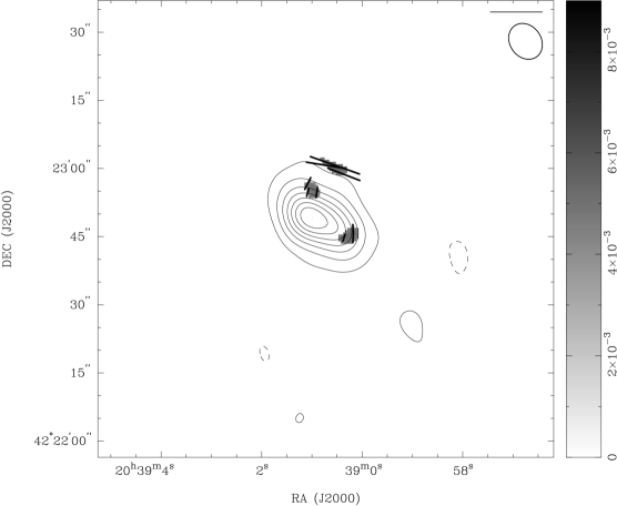
Figure 1: Polarization map of DR21(OH) at 3 mm. The contours represent Stokes I at -0.02, 0.02, 0.04, 0.07, 0.09, 0.11, 0.14, 0.16 and 0.18 Jy beam^-1. The pixel gray scale show $3\sigma$ polarized intensity ($\sqrt{Q^{2}+U^{2}}$) for the dust continuum emission also in Jy beam^-1, while the black vectors are the dust fractional polarization. The length of the vectors are proportional to fractional polarization with the length of the bar at the top-right corresponding to a fractional polarization of 0.33.

Polarization detection is very sensitive to the signal to noise ratio. Because of bad weather conditions during part of our observations we did not achieve the same level of polarization sensitivity as Lai et al. (2003) did. We have 3$\sigma$ polarization detections (figure 1) scattered over 3 positions in the map. The dust polarization detected is consistent with the result of Lai et al. (2003).

2.4 CO $J=1\rightarrow 0$ Observational results

Figure 2 shows the Stokes I spectra integrated over a region that contains the MM1 and MM2 sources (Lai et al., 2003). This region covers the box from RA: 20^h39^m2^s - 20^h38^m59^s.5 to DEC:42^∘22’35” - 42^∘23’2”. Plotted over the Stokes I are the P.A. and the fractional polarization at each velocity channel. The Stokes I spectra generally agree with the CO $J=2\rightarrow 1$ spectra from Lai et al. (2003). In our case the spectrum has a peak at $v_{lsr}=-8$ km s^-1, a minimum at $v_{lsr}=-2$ km s^-1, and a second peak at $v_{lsr}=2$ km s^-1. The velocity of these peaks are different from previous CS and CN observations, which are at -5 km s^-1 (Chandler et al., 1993; Richardson et al., 1994), and -5 km s^-1 and -1 km s^-1 (Crutcher, 1999a). The CO line is optically thick (Figure 2) and the dip, or zero emission range, observed in both CO $J=2\rightarrow 1$ and $J=1\rightarrow 0$ lines, is probably due to self-absorption. In CO $J=1\rightarrow 0$, the dip covers a velocity range from -6 km s^-1 to 2 km s^-1 which coincides with the C³⁴S $J=2\rightarrow 1$ emission peak range from Chandler et al. (1993), which goes from -6 km s^-1 to 1.5 km s^-1. In the same velocity range ¹³CO emission was detected (Dickel et al., 1978) from -3 km s^-1 to 0.5 km s^-1. C³⁴S traces higher densities than CO, and ¹³CO is more optically thin than CO. The presence of peak emission from these lines in the same velocity range of our dip suggests that our CO observations may come from a different region from the higher density gas (which probably comes from the core). Additionally, it is expected that CO polarized line emission will arise from optically thin regions ($\tau\sim 1$) (Goldreich & Kylafis, 1981a; Deguchi & Watson, 1984). Therefore, it is likely that the CO polarized emission that we detected comes from an envelope around DR21(OH).

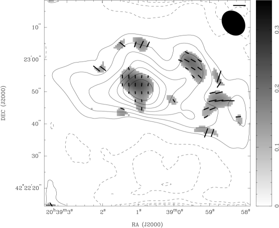
Figure 3: The CO $J=1\rightarrow 0$ polarization emission from DR21(OH) at $v_{lsr}=$-8 km s^-1. The contours represent Stokes I at -6.15, -4.61, -3.08, -1.54, 1.54, 3.08, 4.61, 6.15, 7.7, 9.23, 10.77 and 12.31 Jy beam^-1. The gray scale represents $3\sigma$ polarized emission ($\sqrt{Q^{2}+U^{2}}$) also in Jy beam^-1. The vectors are a representation of the fractional polarization, the length of the bar at the top-right corresponds to a fractional polarization of 0.086. The most widespread polarization pattern occurs at this velocity, which coincides with the peak of the CO emission (Stokes I image).

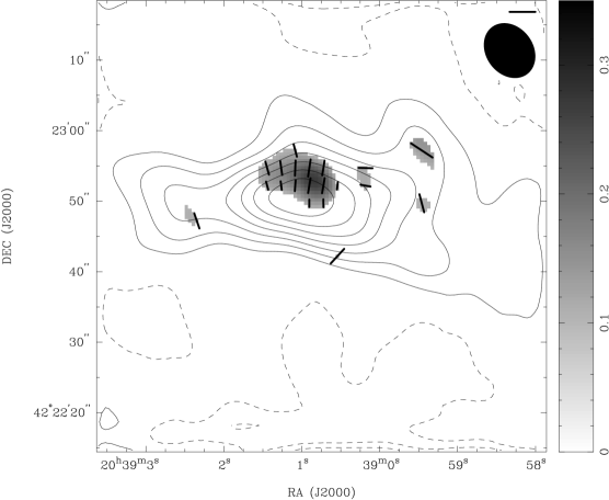
Figure 4: The CO $J=1\rightarrow 0$ polarization emission from DR21(OH) at $v_{lsr}=$-10 km s^-1. The contours represent Stokes I at -2.73, -1.82, -0.91, 0.91, 1.82, 2.73, 3.64, 4.56, 5.47, 6.38 and 7.3 Jy beam^-1. The gray scale represent $3\sigma$ polarized emission ($\sqrt{Q^{2}+U^{2}}$) also in Jy beam^-1. The vectors are a representation of the fractional polarization, the length of the bar at the top-right corresponds to a fractional polarization of 0.064. This map represent the same velocity channel presented by Lai et al. (2003). Comparing with Lai et al. (2003) at the same velocity channel we see that most of the polarization is perpendicular to the CO $J=2\rightarrow 1$ polarization.

Figure 3 shows our CO polarization map at $v_{lsr}=$-8 km s^-1. This map represents the highest significance polarization distribution in our observations. It also coincides with the peak emission of the CO. Figure 4 shows our polarization map at $v_{lsr}=$-10 km s^-1, which is the same velocity map presented by Lai et al. (2003). In our case the $v_{lsr}=$-10 km s^-1 map does not present the same spatial distribution of polarization as the -8 km s^-1 map, almost certainly due to the limited sensitivity of the polarization data. Table 1 gives a comparison between P.A. for both CO transitions. We can see that there is a consistent 90^∘ difference between the transitions.

2.5 Comparison between CO $J=1\rightarrow 0$ and CO $J=2\rightarrow 1$ polarization

Lai et al. (2003) presented a single velocity channel map of their line polarization observations (at $v_{lsr}=-10$ km s^-1); this is the velocity of the peak value in the Stokes I emission. Our CO $J=1\rightarrow 0$ observations have a peak Stokes I at $v_{lsr}=-8$ km s^-1 (Figure 3 ), which also coincides with our most complete polarization spatial distribution.

The Lai et al. (2003) map shows distributed CO emission that is more extensive than the region of the 1.3 mm continuum sources. We see a similar situation in our observations (Figure 3). We also see that our line polarization has better coverage over the CO emission than the Lai et al. (2003) observations (Figure 4). Our observations seem to indicate that with better signal to noise, it might be possible to achieve complete polarization coverage over the region of CO emission. The maximum polarized intensity coincides with the position of the continuum source, a fact which suggests the importance of a continuum radiation field in polarizing the line emission. This was studied in our numerical calculation.

Comparing polarization vectors from Figure 3 and Figure 4 with the map presented by Lai et al. (2003), we found that the P.A. differ; in the central region in both maps most of the P.A. are orthogonal. This is a rather unexpected discovery. The Goldreich - Kylafis effect predicts that polarization can be either parallel or perpendicular to the magnetic field (Goldreich & Kylafis, 1981a), but did not make a distinction between polarization of the same molecule at different transitions. This is because their calculation was done simulating a 2-level molecule. Deguchi & Watson (1984) extended the calculation to a multilevel molecule, but made no prediction about polarization direction in different transitions. Direct comparison of angles in Table 1 shows the $90^{\circ}$ difference between both CO transitions. This is particularly true in the central part of the map.

3 Polarization of molecular lines

3.1 The Goldreich - Kylafis effect

The Goldreich - Kylafis effect is described in a series of papers (Goldreich & Kylafis, 1981a, b; Kylafis, 1983a, b). They considered a molecule with only two (rotational) states having angular momenta $1$ and $0$, and investigated line formation and polarization in the presence of a magnetic field and anisotropic optical depths. Their original work predicted linear polarization up to about ten per cent. Motivated in part by an unsuccessful observational survey for this polarization (Wannier et al., 1983), Deguchi & Watson (1984) extended the calculations to include a number of rotational states and radiative transitions. As a result, the predicted linear polarizations were reduced, typically by a factor of about two. We have further extended the multilevel calculations by including an external source term to represent emission from dust in a compact source. We have also used improved rates for collisional excitation, though this proved to be unimportant. We focus on calculations to understand the polarization angles of the CO $J=2\rightarrow 1$ and $J=1\rightarrow 0$ transitions observed in DR21(OH).

3.2 Basic methods

The formulation used here follows Deguchi & Watson (1984). The radiative transfer equations are solved in the large velocity gradient or Sobolev approximation (hereafter LVG), and in the regime where the line width $\Delta\nu$, the Zeeman splitting $g\mu_{0}B$, and the natural line width $\gamma$ obey the relation $\Delta\nu\gg g\mu_{0}B\gg\gamma$. This strong inequality is easily satisfied here. The quantization $z$ axis is along the magnetic field direction, and the quantum states are specified in the usual way by the total angular momentum $J$ (there is no fine or hyperfine structure here) and by its projection $M$ on the $z$ axis. Under these conditions the radiative transfer equations for radiation associated with transitions between upper state $J$ and lower state $J^{\prime}$ can be written as

$$\frac{dI_{JJ^{\prime}}^{\perp}}{ds}=-\kappa_{JJ^{\prime}}^{\perp}(I_{JJ^{\prime}}^{\perp}-S_{JJ^{\prime}}^{\perp})$$ (1)

$$\frac{dI_{JJ^{\prime}}^{\parallel}}{ds}=-\kappa_{JJ^{\prime}}^{\parallel}(I_{JJ^{\prime}}^{\parallel}-S_{JJ^{\prime}}^{\parallel})$$ (2)

where $\parallel(\perp)$ indicates the intensity of the radiation with a linear polarization parallel (perpendicular) to the magnetic field.

The difference with Goldreich & Kylafis (1981a) comes in expressing the opacity and source terms in a way to allow for arbitrary angular momenta. The opacity and source terms are thus written as $\kappa_{JMJ^{\prime}M^{\prime}}$ and $S_{JMJ^{\prime}M^{\prime}}$ such that $\kappa_{JJ^{\prime}}^{q}$ and $S_{JJ^{\prime}}^{q}$ (where $q$ stands for $\parallel$ or $\perp$),

$$\kappa_{JJ^{\prime}}^{\perp}=\frac{1}{2}\phi(\nu-\nu_{JJ^{\prime}})\sum_{\Delta M=1}\kappa_{JMJ^{\prime}M^{\prime}}$$ (3)

$$S_{JJ^{\prime}}^{\perp}=\frac{\sum_{\Delta M=1}\kappa_{JMJ^{\prime}M^{\prime}}S_{JMJ^{\prime}M^{\prime}}}{\sum_{\Delta M=1}\kappa_{JMJ^{\prime}M^{\prime}}}$$ (4)

$$\kappa_{JJ^{\prime}}^{\parallel}=\phi(\nu-\nu_{JJ^{\prime}})\left(sin^{2}\theta\sum_{\Delta M=0}\kappa_{JMJ^{\prime}M^{\prime}}+\frac{1}{2}cos^{2}\theta\sum_{\Delta M=1}\kappa_{JMJ^{\prime}M^{\prime}}\right)$$ (5)

$$S_{JJ^{\prime}}^{\parallel}=\frac{sin^{2}\theta\sum_{\Delta M=0}\kappa_{JMJ^{\prime}M^{\prime}}S_{JMJ^{\prime}M^{\prime}}+\frac{1}{2}cos^{2}\theta\sum_{\Delta M=1}\kappa_{JMJ^{\prime}M^{\prime}}S_{JMJ^{\prime}M^{\prime}}}{sin^{2}\theta\sum_{\Delta M=0}\kappa_{JMJ^{\prime}M^{\prime}}+\frac{1}{2}cos^{2}(\theta)\sum_{\Delta M=1}\kappa_{JMJ^{\prime}M^{\prime}}}$$ (6)

where the symbol $\theta$ represents the angle between the magnetic field and the direction of propagation and $\kappa_{JMJ^{\prime}M^{\prime}}$ and $S_{JMJ^{\prime}M^{\prime}}$ are defined in terms of Einstein A-coefficients and the populations $n_{JM}$ per magnetic substate

$$\kappa_{JMJ^{\prime}M^{\prime}} =\frac{3}{8\pi}\left(\frac{c}{\nu_{JJ^{\prime}}}\right)^{2}A_{JMJ^{\prime}M^{\prime}}(n_{J^{\prime}M^{\prime}}-n_{JM})$$ (7)

$$S_{JMJ^{\prime}M^{\prime}} =\frac{h\nu_{JJ^{\prime}}^{3}}{c^{2}}\frac{n_{JM}}{n_{J^{\prime}M^{\prime}}-n_{JM}}.$$ (8)

Some equations here differ slightly from those in Deguchi & Watson (1984) because we are treating all magnetic substates explicitly. All statistical weight factors are one and are thus omitted for simplicity.

Since the radiative transfer equations are functions of the populations, rate equations must be solved for these populations. We assume steady state , $\frac{\partial n_{i}}{\partial t}=0$. The rate equations for the populations per magnetic substate are

$$\frac{\partial n_{i}}{\partial t}=-\sum_{j<i}P_{ij}+\sum_{j>i}P_{ji}+\sum_{j}(C_{ji}n_{j}-C_{ij}n_{i})=0$$ (9)

where the $P_{ij}$  (which involve the radiation) are given in terms of the Einstein $A_{JMJ^{\prime}M^{\prime}}$ coefficients and the stimulated emission coefficients $R_{ij}$. The indices $i,j$ correspond to $(J,M),(J^{\prime},M^{\prime})$. The $C_{ij}$ are the collisional excitation rates from state $i$ to state $j$. Deguchi & Watson (1984) used the $C_{ij}$ given by Green & Chapman (1978). In our calculation we have updated the values of $C_{ij}$ with the values provided by Flower (2001), which are given for a wide range of gas temperatures. We used a weighted average for the contribution of ortho and para hydrogen cross sections, specifically, $C_{ij}=0.7\times C_{ij}^{para}+0.3\times C_{ij}^{ortho}$. We considered temperatures up to $T_{gas}=200K$ and angular momenta up to $J=9$. The expressions for the $P_{ij}$ are

$$P_{ij}=A_{ij}[n_{i}+R_{ij}(-n_{j}+n_{i})].$$ (10)

The population equations constitute a nonlinear system, which we solve by numerical iteration.

In the limit in which the macroscopic velocity differences of the gas in the cloud are greater than the thermal velocities of the molecules, the LVG approximation can be used to simplify the solution for the radiative transfer equations. The LVG approximation expresses the intensity as a function of local variables. The intensity that emerges from the gas cloud and is detected by an observer is

$$I_{JJ^{\prime}}^{q}=\left(S_{JJ^{\prime}}^{q}-\frac{B}{2}\right)[1-exp(-\tau_{JJ^{\prime}}^{q})]$$ (11)

where $B$ represents the cosmic background radiation which is included in the calculation, and $\tau_{JJ^{\prime}}^{q}$ is the LVG optical depth for radiation with polarization $q$ at the frequency of the $JJ^{{}^{\prime}}$ transition,

$$\tau_{JJ^{\prime}}^{q}=\kappa_{JJ^{\prime}}^{q}\times L(\theta)$$ (12)

and where $L(\theta)$ is the LVG characteristic scale length for which we adopt the form,

$$L(\theta)=L_{0}/(\alpha\sin^{2}(\theta)+\cos^{2}(\theta)).$$ (13)

When $\alpha<<1,L(\theta)$ reflects a velocity gradient that is perpendicular to the magnetic field; for $\alpha>>1$, the velocity gradient is along the magnetic field (e.g., Deguchi & Watson (1984)). In the calculation, the constant $L_{0}$ enters multiplied by the total number density of CO molecules. We vary this product to obtain the solutions as a function of optical depth that are presented in the Figures.

The $R_{ij}$ in equation 10 involve the integral over frequency and over solid angle of the intensity within the cloud at the location of the CO, and are  non-zero only for $|J-J^{\prime}|=1$, $|M-M^{\prime}|=0$ and $|M-M^{\prime}|=1$ (Deguchi & Watson, 1984),

$$R_{JJ^{\prime}}^{0}=\frac{3c^{2}}{2h\nu^{3}}\int\frac{d\Omega}{4\pi}sin^{2}\theta\int d\nu\phi(\nu-\nu_{JJ^{\prime}})I_{JJ^{\prime}}^{\parallel}(\Omega)$$ (14)

$$R_{JJ^{\prime}}^{1}=\frac{3c^{2}}{4h\nu^{3}}\int\frac{d\Omega}{4\pi}\int d\nu\phi(\nu-\nu_{JJ^{\prime}})[I_{JJ^{\prime}}^{\perp}(\Omega)+cos^{2}\theta I_{JJ^{\prime}}^{\parallel}(\Omega)].$$ (15)

In the LVG approximation the integrals over frequency reduce to

$$\int I_{JJ^{\prime}}^{q}\phi(\nu-\nu_{JJ^{\prime}})d\nu=S_{JJ^{\prime}}^{q}(1-\beta_{JJ^{\prime}}^{q})+\frac{B+S(\Omega)}{2}\beta_{JJ^{\prime}}^{q}$$ (16)

in which the escape probability function is $\beta_{JJ^{\prime}}^{q}=[1-exp(-\tau_{JJ^{\prime}}^{q})]/\tau_{JJ^{\prime}}^{q}$, and S($\Omega$) represents the radiation that is incident from a compact, external continuum source. We express S$(\Omega)$ as

$$S(\Omega)=(1-e^{-\tau_{c}})B_{\nu}(T_{source})$$ (17)

for directions $\Omega$ that are subtended by the external source as viewed from the location of the CO. In other directions, S$(\Omega)=0$. In equation 17, B${}_{\nu}(T_{source})$ is the Planck function, $T_{source}$ is the source temperature, and $\tau_{c}$ is the continuum optical depth of the source at the relevant frequency. We adopted the parameterization of Mangum et al. (1991) for the combined emission from the dust core of DR21(OH), specifically, T${}_{source}=42$ K, $\tau_{c}$=1.5$[0.25/\lambda[mm]]^{2}$ and an effective source angular size (radius) of 10^′′ as seen from the earth. At the location of the CO, the angular size (radius) for the source is then approximately 1/2 radian (assuming 0.3 pc for the separation between the CO and the source). Finally, the fractional polarization is expressed as

$$P=\frac{I_{\perp}-I_{\parallel}}{I_{\perp}+I_{\parallel}}.$$ (18)

3.3 Calculation results

The objective of this calculation is to understand why the the directions of the polarizations for the CO $J=1\rightarrow 0$ and the CO $J=2\rightarrow 1$ radiation are perpendicular to one another in the DR21(OH) observations described in Section 2, with the $J=1\rightarrow 0$ polarization parallel to that of the emission by the dust grains. We want to calculate the linearly polarized radiation emitted by CO for physical conditions that are representative for the DR21(OH) star forming region, and determine whether the observed directions and magnitudes of the polarization can be reproduced. The orthogonality of the polarizations is reflected by a sign difference in $P$ in equation 18 . If $P>0$, $I_{\perp}$ dominates the emission and the polarization is perpendicular to the magnetic field. In the other case it is parallel.

The physical conditions for our multilevel calculation are described below. These conditions are consistent with the assumption that the polarized emission comes from a cold envelope around the DR21(OH) continuum sources. We assumed that the physical conditions are the same in the gas for both CO transitions.

To obtain a qualitative understanding of how the polarizations can be orthogonal for the two transitions, consider the $J=1\rightarrow 0$ transition by itself, and first without any external radiation.  If the velocity gradients are smaller in directions parallel to the magnetic field than in directions perpendicular to the magnetic field,  the optical depths for spectral lines will be the largest parallel to the field lines.  The escape of radiation involved in de-exciting the upper $J=1$ state will then be reduced more in directions along the field lines than in directions perpendicular to the field lines. This in turn leads to populations of the $M=\pm 1$ substates that are larger than the populations of the $M=0$ substate because of the difference in the angular distributions of the de-exciting radiation. The angular distribution of the $\sigma$ radiation ($\left|M-M\acute{}\right|$ $=1$ transitions) peaks in directions along the field lines whereas that of the $\pi$ radiation ($\left|M-M\acute{}\right|$ $=0$ transitions) peaks in directions perpendicular to the magnetic field. Hence, when the velocity gradients are smallest along the magnetic field, the rate for de-excitation of the $M=\pm 1$ substates is decreased more by trapping of the radiation than is the de-excitation rate of the $M=0$ substate . The excitation rate for all magnetic substates by collisions is the same. Under isotropic conditions, the populations of the magnetic substates are equal. For any direction, the $\sigma$ and $\pi$ radiation that emerges from the radiative decays of these states will combine to give zero net polarization. However, when the $M=\pm 1$ states have larger populations, the $\sigma$ radiation will be relatively stronger in comparison with the $\pi$ radiation. Their contributions to the polarization will not then cancel and the combined radiation will be linearly polarized—in the direction of the polarization of the $\sigma$ radiation which is perpendicular to the magnetic field.

Now consider by itself a compact, external source of radiation (i. e., no anisotropy in the optical depths as in the above paragraph) that is located in a direction perpendicular to the magnetic field. Because the angular distribution associated with $\pi$ transitions is larger for this direction than is the angular distribution of the $\sigma$ transitions, the $J=1,M=0$ substate will be excited more rapidly by absorption of this radiation than will be the $J=1,M=\pm 1$ substates. The $J=1,M=0$ substate would then become overpopulated in comparison with the other two magnetic substates and radiation that emerges from the gas would be polarized in the direction of $\pi$ radiation—parallel to the magnetic field.

Though the reasoning is more complicated because of the additional substates and transitions, analogous conclusions apply for the polarization of the radiation associated with the $J=2\rightarrow 1$ and higher transitions of the CO molecule.

When the above anisotropic velocity gradients and external source of radiation are both present, the direction of the polarization of the radiation that is emitted by the gas is determined by the relative importance of these two causes of anisotropy. Their relative importance is not, however, the same for the $J=2\rightarrow 1$ as for the $J=1\rightarrow 0$ transition. The dust radiation from the core of DR21(OH) is much higher at the CO $J=2\rightarrow 1$ transition frequency than the CO $J=1\rightarrow 0$ frequency, and thus the external radiation will play a greater role for the polarization of the $J=2\rightarrow 1$ transition than it does for the $J=1\rightarrow 0$ transition. The effect of the anisotropic velocity gradients is about the same for the two transitions since the collisional excitation rates are about the same for both transitions (the excitation energies for these states of CO are less than $kT_{gas}$). The $J=2\rightarrow 1$ radiation can then reflect the influence of the radiation and be polarized parallel to the magnetic field under conditions for which the $J=1\rightarrow 0$ radiation reflects the influence of the velocity gradient and is polarized perpendicular to the magnetic field. The results presented below from the numerical calculations demonstrate that this orthogonality in the polarizations occurs for physical conditions that are likely for the gas that is emitting the polarized CO radiation from DR21(OH). Velocity gradients that are anisotropic and systematically larger in the direction perpendicular to the magnetic field occur in magnetohydrodynamic turbulence (see Watson et al. (2004))

Calculations were performed for gas temperatures between 15 and 50 K and for a range of densities. Dickel et al. (1978) obtained a T_gas=28 K; this temperature is used as a reference for our calculations. The velocity gradient must be largest in the direction perpendicular to the magnetic field according to the above reasoning. We thus focus on $\alpha=0.1$ in the expression for $L(\theta)$, though we also present results for $\alpha$=0.3 for comparison.

Three curves for polarization versus LVG optical depth that correspond to calculations with densities $n_{H_{2}}=$ 25, 75 and 225 cm^-3 are shown in Figure 5 for $T_{gas}=28$ K. These densities are in agreement with what we might expect in a lower density envelope. Padin et al. (1989) obtained a $n_{H_{2}}$ density of $n_{H_{2}}=5\times 10^{6}$ cm^-3, but this corresponds to the MM1 continuum source and not to the DR21(OH) envelope. At the lowest optical depths, the external continuum source dominates in determining the direction of the polarization for both transitions whereas at the highest optical depths this radiation is largely excluded and the velocity gradient determines the direction of the polarization for both transitions. However, because the continuum emission from the core of DR21(OH) is much higher at the frequency of the $J=2\rightarrow 1$ transition than at the frequency of the $J=1\rightarrow 0$, the external radiation remains more important to higher optical depths for the $J=2\rightarrow 1$ transition than for the $J=1\rightarrow 0.$ Hence, a range of optical depths occurs over which the polarizations are orthogonal. This range of optical depths is mostly from $\log(\tau)\simeq 0$ to $-1$ in Figure 5. In this range of optical depths, the fractional polarizations typically are a few percent and are thus consistent with the observed magnitudes for the fractional polarizations of the two transitions. These small $\tau$ values are consistent with our assumption that the polarized CO emission arises from a cold, low density gas, which in turn is compatible with the likely conditions for the DR21(OH) envelope. At the highest optical depths, the fractional polarization tends to zero in Figure 5 for both transitions as expected. The polarizations in the second panel in Figure 5 (for $\alpha$=0.3) provide an indication of the sensitivity of the calculations to the magnitude of the velocity gradients. The polarizations for both transitions are presented only as a function of the CO $J=1\rightarrow 0$ optical depth. However, the CO $J=2\rightarrow 1$ optical depth is similar in our calculations.

The curves in Figure 5 correspond to the densities that represent our best results. Our calculations show that for densities over n${}_{H_{2}}$=500 cm^-3 the fractional polarization decreases dramatically for both lines, vanishing almost completely for densities over n${}_{H_{2}}$=1000 cm^-3. At the higher densities collisions are more rapid and the continuum source is no longer an important source of anisotropy. On the other hand, densities below n${}_{H_{2}}$=20 cm^-3 would require an envelope too big and far away from the continuum source, which would make the central continuum source ineffective as an additional source of anisotropy.

In Figure 6, we demonstrate explicitly that the polarization is positive for both transitions at all optical depths in our calculations when there is no continuum source so that the velocity gradients determine the direction of the polarization. The fractional polarization also tends to zero at large and at small optical depths as expected, and as found by the previous investigators.

In Figure 7, we present the results of our calculations for the other extreme; the limit in which the radiation from the continuum source dominates. We cannot eliminate collisions completely in our calculations. However, we can greatly reduce their influence by multiplying the collision rates by a small factor (10^-5). As expected, the polarization is now negative for both lines (parallel to the magnetic field), is independent of density and converges to zero for higher optical depths.

In our calculations, we also varied the gas temperature in order to explore the influence of uncertainty about the gas temperature in the envelope around DR21(OH). We found no significant variation in the polarizations for $T_{gas}$ between 15 and 50 K. What we found is that the range in $\tau$ for which the polarizations are orthogonal shifts slightly in $\tau$; there is a displacement to lower $\tau$ for higher temperatures. A molecular envelope might be heated by external UV photons or cosmic rays. This insensitivity to gas temperature shows a degree of robustness for the results of our calculations. We have also verified that the results are insensitive to the temperature of the dust by performing computations with $T_{source}$ up to 60 K.

The polarizations presented in Figures 5-7 are for the radiation that is emitted by the gas at an angle of 90^∘ with respect to the magnetic field. We have verified that the polarization characteristics are similar for emission at angles from 90^∘ to about 40^∘. At smaller angles, the polarized fraction decreases significantly—approaching zero at 0^∘, as expected.

3.4 Magnetic field strength and cloud support

Our work has shown that the line polarization will trace magnetic field geometry at lower densities than the dust polarization. However, comparing with the results of Lai et al. (2003), we believe that there is a correlation between the field traced by the dust (core) and the field traced by the line (envelope). Our dust polarization result at 3 mm shows similar P.A. to the 1.3 mm dust polarization of Lai et al. (2003). Also we now know why the line polarizations are perpendicular at two different transitions, which makes the CO $J=1\rightarrow 0$ polarization consistent with the CO $J=2\rightarrow 1$. At different frequencies the line polarization is either parallel or perpendicular to the dust polarization. The agreement in the geometries of the dust and line polarization suggests that the field in the core and the envelope are connected and not independent.

Lai et al. (2003) estimated the magnetic field strength to be about 0.9 mG for MM1 (n${}_{H_{2}}\sim 1\times 10^{6}$ cm^-3) and 1.3 mG for MM2 (n${}_{H_{2}}\sim 2\times 10^{6}$ cm^-3). Crutcher (1999a) measured a magnetic field in the line of sight $B_{los}\sim$ -0.4 mG for MM1 and $B_{los}\sim$ -0.7 mG for MM2. Chandrasekhar & Fermi (1953) predicted a magnetic field dependence proportional to $\rho^{1/2}$

$$B_{ChF}=Q\sqrt{4\pi\rho}\frac{\Delta v_{los}}{\Delta\phi}$$ (19)

The dispersions in the measured velocities and P.A. are similar for the $J=1\rightarrow 0$ and $J=2\rightarrow 1$ lines. Therefore, we can extrapolate the values of the magnetic field measured in the core to the envelope following a $\rho^{1/2}$ law. The molecular hydrogen number density for the cores is in the order of n${}_{H_{2}}$ = 10⁶ cm^-3, and taking a density of n${}_{H_{2}}$ = 100 cm^-3 for the envelope, we get a magnetic field in the envelope 100 times smaller than the core value of $\sim$ 1 mG (at n${}_{H_{2}}\sim 1\times 10^{6}$ cm^-3), or about 10 $\mu G$. We can use this value to estimate the mass to magnetic flux ratio; its critical value is given by (Mouschovias & Spitzer, 1976)

$$\frac{M}{\Phi_{B}}_{crit}=\frac{1}{\sqrt{63G}}$$ (20)

This equation can be expressed as a function of volume density in an spherical model, using the molecular hydrogen mass, equation 20, and expressing the magnetic field in G units, and the distance in cm. We arrived at

$$\frac{M/\Phi}{M/\Phi}_{crit}=9.1\times 10^{-27}\frac{R[cm]\times n[cm^{-3}]}{B[G]}$$ (21)

in which R is the radius of the cloud, $n$ is the number density of hydrogen molecules and B is the magnetic field. Using a density $n=$100 cm^-3, $B$=10 $\mu$G and a radius of R=0.3 pc, we obtained a mass-to-flux ratio of 0.13 times the critical value, and thus highly subcritical. Hence, the envelope is supported against gravitational contraction by the magnetic field. The value of R represents an angular distance of 0.3 pc of distance for DR21(OH). This radius may be underestimated due to resolution of more extended structure by the interferometer. However, single dish maps (Wilson & Mauersberger, 1990) suggest that R $<$ 1 pc.

4 Summary and conclusions

DR21(OH) was observed in 3 mm dust continuum and CO $J=1\rightarrow 0$ line emission. Comparing our line observations with Lai et al. (2003), we observed a consistent difference in polarization direction between the CO $J=2\rightarrow 1$ and CO $J=1\rightarrow 0$ lines; they are perpendicular to each other over the central region (which coincides with the position of the MM1 and MM2 continuum sources). We developed a code based on the Deguchi & Watson (1984) calculation in order to solve the radiative transfer equations and calculate the fractional linear polarization for different transitions of the CO molecule. We found that the presence of a small continuum source will likely produce an increase in the anisotropy of the radiation field over the CO gas. An anisotropic radiation field will unevenly populate the magnetic sub-levels of the CO molecule, which will produce linearly polarized emission. We showed that the presence of a compact continuum source will produce a gradual change in the fractional polarization, with a sign change, as a function of optical depth. This would explain the orthogonal orientations of the CO polarization in different transitions. In the particular case of DR21(OH), the physical conditions that are consistent with the polarization data correspond to a hot continuum source ($T_{dust}$ $\sim$ 42 K) and a CO gas temperature of $T_{gas}\sim$ 28 K, for a $n_{H_{2}}\sim$100 cm^-3.

Line polarization observations can become a powerful tool to constrain the magnetic field geometry. We have seen that a clear understanding of the physical conditions in a molecular cloud will give more accurate information about the fractional polarization sign. A good knowledge of the sources of anisotropy in a cloud will help to understand and constraint the geometry in line polarization observations at multiple frequencies.

We also found that line polarization traces low density material; this is important in order to connect the magnetic field geometries at different densities. In the particular case of DR21(OH) we believe that there may be a correlation between the field traced by the dust at densities of 10⁶ cm^-3 and the field traced by line polarization at 10² - 10³ cm^-3. However, we were only able to compare our calculation with polarization observations of CO molecular transitions. We believe that polarization information from additional molecules may probe the magnetic field geometry at intermediate densities giving a more accurate picture of the field morphology in star forming regions.

Having information about the magnetic field at different densities is useful to test the gravitational state of equilibrium for the cloud. Polarization mapping can allow the Chandrasekhar-Fermi method to be used to obtain an estimate of the magnetic field strength and test whether the envelope is magnetically supported or not. The envelope of DR21(OH) appears to be magnetically supported.

This research has been supported partially by NSF grants AST 02-05810 and AST 99-88104.

Table 1: Position angle for CO $J=2\rightarrow 1$ and CO $J=1\rightarrow 1$ at velocity channel map $v=$ -10 km s^-1. Data was interpolated at a tolerance of 0.2^′′ that corresponds to approximate 2.7 $\times$ 10^-4 pc using a distance to DR21(OH) of 3 kpc.

Offsets in arcsec	$\phi_{J=2\rightarrow 1}$	Offsets in arcsec	$\phi_{J=1\rightarrow 0}$
(1.0,2.0)	78$\pm$5	(1.0,2.0)	3.6$\pm$9.2
(-0.6,2.0)	77$\pm$5	(-0.6,2.0)	4$\pm$9.6
(4.2,4.0)	87$\pm$7	(4.0,4.0)	-0.2$\pm$8.9
(2.6,4.0)	85$\pm$6	(2.5,4.0)	-5.2$\pm$6.2
(1.0,4.0)	83$\pm$7	(1.0,4.0)	-6.1$\pm$5.3
(-0.6,4.0)	84$\pm$7	(-0.5,4.0)	-4.6$\pm$6.2
(9.0,6.0)	-60$\pm$5	(9.0,6.0)	15.3$\pm$9.7
(7.4,6.0)	-70$\pm$6	(7.5,6.0)	13.0$\pm$7.6
(5.8,6.0)	-85$\pm$8	(6.0,6.0)	6.7$\pm$6.9
(4.2,6.0)	88$\pm$8	(4.2,6.0)	-3.5$\pm$5.5
(2.6,6.0)	87$\pm$8	(2.5,6.0)	-9.3$\pm$4.1
(9.0,8.0)	-50$\pm$7	(9.0,8.0)	18.4$\pm$9.6
(7.4,8.0)	-62$\pm$8	(7.5,8.0)	14.1$\pm$7.6
(5.8,8.0)	-76$\pm$9	(6.0,8.0)	8.0$\pm$6.6

Figure 2: The spatially averaged Stokes I spectrum from the CO $J=1\rightarrow 0$ emission. We observe a peak of 5.6 Jy beam^-1 at $v_{lsr}=-8$ km s^-1, while the minimum is located at $v_{lsr}=-2$ km s^-1. (upper panel). Plotted over is the averaged P.A. over the Stokes I spectrum. Most of the velocity channels have P.A. that are orthogonal to the Lai et al. (2003) result. (lower panel) The integrated fractional polarization is plotted over the Stokes I spectrum.

Figure 5: Fractional polarization $P$ calculated for the CO transitions $J=1\rightarrow 0$ and $J=2\rightarrow 1$ as a function of the LVG optical depth for the CO $J=1\rightarrow 0$ transition. Here, $T_{gas}=$28 K and $T_{source}=$42 K. Each pair of curves represents calculations for a different density of molecular hydrogen—25 cm^-3, 75 cm^-3 and 225 cm^-3. In the upper panel, the velocity gradient is characterized by $\alpha$=0.1. In order to test the robustness of the calculation, we decreased the degree of anisotropy by setting $\alpha$=0.3. This is shown in the lower panel.

Figure 6: Fractional polarizations $P$ calculated for the CO transitions $J=1\rightarrow 0$ and $J=2\rightarrow 1$ are shown as a function of $\tau$ for the molecular hydrogen densities 25, 75 and 225 cm^-3 when there is no compact, external source of continuum radiation. Here, the direction of the polarizations is determined by the direction of the velocity gradient and is perpendicular to the direction of the magnetic field. Note that the polarizations of the CO $J=1\rightarrow 0$ and $J=2\rightarrow 1$ transitions are never orthogonal (i. e. they always have the same sign.)

Figure 7: Fractional polarization $P$ for the CO transitions $J=1\rightarrow 0$ and $J=2\rightarrow 1$ are shown as a function of $\tau$ when the collision rates used in Figure 5 are reduced by multiplying by a factor 10^-5. For the relevant hydrogen densities (25 - 225 cm^-3), the external continuum source dominates in determining the direction of the polarization for both transitions and the polarizations do not depend on density. For both spectral lines, the polarization is parallel to the magnetic field (negative sign) as expected, and converges to zero for large values of $\tau$.

References

- Barvainis & Wooten (1987) Barvainis, R., & Wooten, A., 1987. AJ, 93, 168
- Batrla & Menten (1988) Batrla, W., & Menten, K., M., 1988. ApJ, 329, L117
- Chandrasekhar & Fermi (1953) S., Chandrasekhar, E., Fermi, 1953. ApJ, 118, 113
- Crutcher (1999b) R., M., Crutcher 1999. ApJ, 520, 706
- Crutcher (1999a) R., M., Crutcher, T., H., Troland, B., Lazaref, G., Paubert, & I. Kazes, 1996. ApJ, 456, 217
- Chandler et al. (1993) Chandler, C., Moore, T., Gear, W., K., Chini, R., 1993, MNRAS, 260, 337.
- Chandler et al. (1993) Chandler, C., Moore, T., Mountain, C., Yamashita, T., 1993, MNRAS, 261, 694.
- Deguchi & Watson (1984) Deguchi, S., Watson, W., D., 1984. ApJ, 185, 126
- Dickel et al. (1978) Dickel, H., Dickel, J., Wilson, W., 1978, ApJ, 223, 840.
- Flower (2001) Flower, D., R., 2001, J.Phys.B., 34, 2731
- Gear et al. (1988) Gear, W., K., Chandler, C., J., Moore, T., J., T., Cunningham, C., T., Duncan, W., D., 1988. MNRAS, 231, 47
- Genzel & Downes (1977) Genzel, R., & Downes, D., 1977. A&AS, 30, 145
- Girart & Crutcher (1999) Girart, J., M., Crutcher, R., M.& Rao, R., 1999, ApJ, 525, L109.
- Glenn et al. (1987) Glenn, J., Walker, C., Jewell, P., 1997, ApJ, 479, 325
- Goldreich & Kylafis (1981b) Goldreich, P., Kylafis, N. 1981. ApJ, 253, 606
- Goldreich & Kylafis (1981a) Goldreich, P., Kylafis, N. 1980. ApJ, 243, L75
- Greaves et al. (1999) Greaves, J., Holland, W., Friberg, P. 1990. ApJ, 512, L139
- Green & Chapman (1978) Green, S., Chapman, S. 1978. ApJS, 37, 169
- Harvey et al. (1986) Harvey, J., A., Ruderman, M., A., & Shaham, J., 1986. Phys. Rev. D, 33, 2084
- Hasegawa et al. (1991) Hasegawa, T., Mitchell, G., & Henriksen, R ., 1991. AJ, 102, 666
- Johnston et al. (1984) Johnston K., J., Heinkel, C., & Wilson, T., L., 1984. ApJ, 285, L85
- Kylafis (1983a) Kylafis, N. 1983. ApJ, 267, 137
- Kylafis (1983b) Kylafis, N. 1983. ApJ, 267, 137
- Lai et al. (2001) Lai, S., P., Crutcher, R., M., Girart, J., M., & Rao, R., 2001, ApJ, 561, 864.
- Lai et al. (2002) Lai, S., P., Crutcher, R., M., Girart, J., M., & Rao, R., 2002, ApJ, 566, 925.
- Lai et al. (2003) Lai, S., Girart, J., M., Crutcher R., M., 2003. ApJ, 598, 392
- Langer & Penzias (1990) Langer, W., & Penzias, A. 1990. ApJ, 357, 477
- Lazarian (2003) Lazarian, A., 2003, QJSRT, 79, 88
- Lis et al. (1988) Lis, D., C., Goldsmith, R., Predmore, C., Omont, A. & Cernicharo, J., 1988. ApJ, 328, 304
- Mangum et al. (1991) Mangum, J., G., Wootten, A., & Mundy, L., G., 1992. ApJ, 378, 576
- Minchin et al. (1994) Minchin, N., & Murray, A., 1994. A&A, 286, 579
- Minchin et al. (1995) Minchin, N., White, G., & Ward-Thompson, D., 1995. A&A, 301, 894
- Minchin et al. (1996) Minchin, N., Bonifacio, V., Murray, A., 1996. A&A, 315, L5
- Mouschovias & Spitzer (1976) Mouschovias, T., Ch. & Spitzer, L. 1976. ApJ, 210, 326
- Norris et al. (1982) Norris, R., P., Booth, R., S., Diamond, P., J., & Porter, N., D., 1982, MNRAS, 201, 191
- Padin et al. (1989) Woody, D., P., Scott, S., L., Scoville, N., Z., Mundy, L., G., Sargent, A., I., Padin, S., Tinney, C., G., & Wilson, C., D., 1989. ApJ, 337, L41
- Plambeck & Menten (1990) Plambeck, R. L., Menten, M. N., 1990, ApJ, 364, 555.
- Rao et al. (1998) Rao, R., Crutcher, R., M., Plambeck, R., L., & Wright, M., C., H., 1998, ApJ, 502, L75.
- Richardson et al. (1994) Richardson, K., J., Sandell, G., Cunningham, C., T., & Davis, S., R., 1994, A&A, 286, 555
- Sault & Kileen (1995) R. J. Sault, N. E. B. Killeen, Miriad Users Guide
- Townes & Schawlow (1955) Townes, C., H., & Schawlow, A., L., 1955. Microwave spectroscopy (New York, McGraw-Hill)
- Wannier et al. (1983) Wannier, P., G., Scoville, N., Z., and Barvainis, R. 1983. ApJ, 267, 126
- Watson et al. (2004) Watson, W., D., Wiebe, D., S., McKinney, J., C., & Gammie, C., F., 2004. ApJ, 604, 707
- Williams et al. (1974) Wannier, P., G., Scoville, N., Z., and Barvainis, R. 1983. ApJ, 267, 126
- Wilson & Mauersberger (1990) Wilson, T., L., Mauersberger, R., 1990. A&A, 239, 305
- Woody et al. (1989) Woody, D., P., Scott, S., L., Scoville, N., Z., Mundy, L., G., Sargent, A., I., Padin, S., Tinney, C., G., & Wilson, C., D., 1989. ApJ, 33 7, L41