Detection of satellite remnants in the Galactic Halo with Gaia – I. The effect of the Galactic background, observational errors and sampling

Abstract

We address the problem of identifying remnants of satellite galaxies in the halo of our galaxy with Gaia data. The Gaia astrometric mission offers a unique opportunity to search for and study these remnants using full phase-space information for our Galaxy’s halo. However, the remnants have to be extracted from a very large data set (of order $10^{9}$ stars) in the presence of observational errors and against a background population of Galactic stars. We address this issue through numerical simulations with a view towards timely preparations for the scientific exploitation of the Gaia data.

We present a Monte Carlo simulation of the Gaia catalogue with a realistic number of entries. We use a model of the galaxy that includes separate light distributions and kinematics for the bulge, disc and stellar halo components. For practical reasons we exclude the region within Galactic coordinates: $-90^{\circ}\leq\ell\leq 90^{\circ}$ and $-5^{\circ}\leq b\leq 5^{\circ}$, close to the Galactic plane and centre. Nevertheless, our catalogue contains $3.5\times 10^{8}$ stars. No interstellar absorption has been modelled, as we limit our study to high Galactic latitudes.

We perform tree code $10^{6}$–body simulations of satellite dwarf galaxies in orbit around a rigid mass model of the Galaxy. We follow the simulations for $10^{10}$ years. The resulting shrinking satellite cores and tidal tails are then added to the Monte Carlo simulation of the Gaia catalogue. To assign photometric properties to the particles we use a Hess diagram for the Solar neighbourhood for Galactic particles, while for the dwarf galaxy particles we use isochrones from the Padova group. When combining the Milky Way and dwarf galaxy models we include the complication that the luminosity function of the satellite is probed at various depths as a function of position along the tidal tails. The combined Galaxy and satellites model is converted to a synthetic Gaia catalogue using a detailed model for the expected astrometric and radial velocity errors, depending on magnitude, colour and sky position of the stars.

We explore the feasibility of detecting tidal streams in the halo using the energy versus angular momentum plane. We find that a straightforward search in this plane will be very challenging. The combination of the background population and the observational errors will make it difficult to detect tidal streams as discrete structures in the $E$–$L_{z}$ plane. In addition the propagation of observational errors leads to apparent caustic structures in the integrals of motion space that may be mistaken for physical entities. Any practical search strategy will have to use a combination of pre-selection of high-quality data and complementary searches using the photometric data that will be provided by Gaia.

Table 1: Scientific capabilities of the Gaia mission. Listed are the survey parameters and the measurements with their expected accuracies. Note that $\mu$arcsec stands for micro-arcsecond. The numbers in this table are from the Gaia Concept and Technology Study Report (see ESA, 2000; Perryman, 2002)

Survey parameters		Measurements and accuracies
Magnitude limit	20–21 mag	Astrometry	4 $\mu$arcsec at $V=10$
Completeness	20 mag		11 $\mu$arcsec at $V=15$
Number of objects	26 million to $V=15$		160 $\mu$arcsec at $V=20$
	250 million to $V=18$	Photometry	4 broad band to $V=20$
	1000 million to $V=20$		11 medium band to $V=20$
Observing programme	On-board and unbiased	Radial velocities	1–10 km s-1 at $V=16$–$17$

1 Introduction

Current cosmological models for the formation of the large scale structure of the Universe envisage the formation of large luminous galaxies as a long process of merging of smaller structures (Kauffmann & White, 1993). Although the details that lead from the merging of dark haloes to the formation of luminous galaxies are quite complicated and currently addressed only through the use of semi–analytical models (Kauffmann, White & Guiderdoni, 1993; Somerville & Primack, 1999; Cole at al., 2000), it is clear that such a formation scenario must have left an imprint on the halo of luminous galaxies like ours, where the long dynamical time scales preserve for a long time the remnants of old mergers (Lynden-Bell, 1976). Although with low statistical weight due to the small number of stars involved, for a long time there has been increasing evidence of the existence of substructure in the stellar halo of our galaxy (Eggen, 1965; Rodgers & Paltoglou, 1984; Ratnatunga & Freeman, 1985; Dionidis & Beers, 1989; Arnold & Gilmore, 1992; Majewski, Munn & Hawley, 1996). This trend culminated with the discovery of the Sagittarius Dwarf galaxy by Ibata, Gilmore & Irwin (1994) and the discovery of the Canis Major dwarf (Newberg et al., 2002; Martin et al., 2004). These satellite galaxies are in the process of being torn apart by the tidal field of our Galaxy.

The identification and study of substructure in our stellar halo is of paramount importance, not only because it traces the formation of our Galaxy, but because it allows us to probe the clustering of dark matter at small spatial scales (for a recent review see Freeman & Bland-Hawthorn, 2002). This clustering is a crucial clue to the nature of its constituents: The nature of the dark matter sets the scale at which dark matter can clump (Bond & Szalay, 1983; Navarro, Frenk & White, 1997; Klypin et al., 1999; Moore et al., 1999). A popular current candidate, the axion, is “cold” enough that it can clump at scales of dwarf galaxies. Although evidence for dark matter within dwarf galaxies orbiting our galaxy has been put forward (Irwin & Hatzidimitriou, 1995), this evidence is weakened by the unfortunate degeneracy between potential well depth and orbital eccentricity in the dynamical models (Wilkinson et al., 2002). Identification and modelling of several satellite systems in the process of being torn apart by the tidal field of our galaxy can help to disentangle this degeneracy, as the rate of erosion of the satellite depends more importantly on the depth of its own potential well than on the details of its internal dynamics (Roche Lobe argument, Mihalas & Binney, 1981).

Several authors have pointed out that the thick disc of our galaxy may have been produced by a merger event around 10 Gyr ago (Gilmore & Wyse, 1985; Carney, Latham & Laird, 1989). Wyse (1999) has pointed out that this corresponds to a redshift of $z\sim 2$. By probing the structure that exists within the halo of our galaxy, we are doing ‘in situ’ cosmological studies of events that took place long ago. Recent observations (Stockton, Canalizo & Maihara, 2004; Tecza et al., 2004) have shown evidence for the existence of luminous galaxies at large redshifts ($z\sim 2.5$) that seem to be old, massive and have large metallicity. Their existence in large numbers, if confirmed, poses a challenge to the standard cosmological scenario of bottom-up formation. It is clear that it is of paramount importance to study the stratigraphy of the halo of our galaxy to try to discern what the assemblage process was by which our galaxy arose.

Great progress has recently been made in the study of sub-structure in the halo of the Milky Way through dedicated surveys of halo giants and other tracer populations (e.g., Morrison et al., 2000; Majewski et al., 2000; Palma et al., 2003). In addition large scale photometric surveys, such as SDSS and 2MASS (York et al., 2000; Cutri et al., 2003) which cover the entire sky or large parts thereof, have been exploited to explore the halo substructure (e.g., Newberg et al., 2002; Martin et al., 2004; Rocha-Pinto et al., 2004). However all these surveys provide at most one component of the space motion for a very small fraction of the stars surveyed and often they only probe a small fraction of the halo. To definitively unravel the structure and formation history of the Galactic halo (and the Galaxy as a whole) detailed phase-space information is required of a significant fraction of the entire volume of the Galactic halo (Freeman & Bland-Hawthorn, 2002). This requires a very high precision astrometric survey done over the whole sky, complemented with radial velocities and photometry.

In 2000 October the Gaia satellite mission was selected as the European Space Agency’s sixth Cornerstone mission to be launched no later than 2012. The main scientific aim of the Gaia mission is to map the structure of the Galaxy and unravel its formation history by providing a stereoscopic census of 1 billion stars throughout the Galaxy. This will be achieved by measuring accurate positions, parallaxes and proper motions for all stars to a limiting magnitude of $V=20$. To complement the astrometric information radial velocities will be collected for all stars brighter than $V\simeq 17$. In addition photometry will be measured for all stars; four broad bands will be employed and about 11 intermediate bands, which will provide detailed astrophysical information for each detected object. Gaia will employ an on-board detection scheme allowing it to measure every detected object brighter than $V=20$. This ensures an unbiased and complete survey of the Galaxy. The scientific capabilities of Gaia are summarized in Table 1. For details see Perryman (2002), Perryman et al. (2001), and ESA (2000).

These measurement accuracies can be put into perspective by using Galaxy models to calculate the corresponding distance and tangential velocity accuracies (see Perryman, 2002): 21 million stars will have distances with a precision better than 1 per cent, 116 million better than 5 per cent and 220 million better than 10 per cent; 84 million stars will have tangential velocities with a precision better than $1$ km s^-1, 210 million better than $3$ km s^-1, 300 million better than $5$ km s^-1, and 440 million better than $10$ km s^-1.

In view of this kind of stereoscopic data becoming available for the Galaxy in the future, several authors have made simulations of the process of accretion and tidal disruption of satellite galaxies in the halo of our galaxy, with the goal of identifying the characteristics of the resulting debris (e.g. Oh, Lin & Aarseth, 1995; Johnston, Hernquist & Bolte, 1996; Meza et al., 2005). Helmi & White (1999), and Helmi & de Zeeuw (2000), in particular, have studied the problem of identifying the resulting substructure in the stellar halo with information from a new generation of astrometric space missions. They conclude that a promising technique is to search for this substructure using conserved dynamical quantities: energy and angular momentum. They performed simulations of the destruction and smearing of satellite galaxies in the halo of our galaxy and plotted the remnants in the $(E,L,L_{z})$ space. They applied a simple model of the astrometric errors expected in the FAME, DIVA and Gaia missions, that depends on the apparent magnitude alone. The errors for the Gaia mission will depend also on the Ecliptic coordinates and the colour of stars, and this can introduce additional correlations between the astrometric variables. In addition Helmi & de Zeeuw (2000) only considered relatively bright and nearby ($V\la 15$, $d\la 6$ kpc) stars when constructing their $E$–$L$–$L_{z}$ diagrams. However, when searching for substructure throughout the whole volume occupied by the Galaxy’s halo, the majority of stars will be much fainter (and much further away) and have correspondingly worse astrometric errors (see Table 1) which will result in much more smearing in the $(E,L,L_{z})$ space. Finally, previous investigations have not taken into account the problem of contamination by the Galactic background. It is expected that, in any given field, the signature of an accretion event will not dominate the corresponding star counts and a method should be devised to identify the proverbial ‘needle in the haystack’.

The goals of this work are to:

1. understand, through simulations, how one can detect and trace the debris of disrupted satellites in the halo of our galaxy using direct measurements of phase-space, as will be provided by Gaia.

2. include a realistic model of the Galactic background population against which the remnants have to be detected. This includes a more elaborate model of the observational errors expected for Gaia.

3. gain practical experience with analysing and visualizing the enormous volume of multi-dimensional information that will be present in the Gaia data base.

For the Galaxy model we have been careful to use Monte Carlo simulations that result in the expected number of stars in the Gaia catalogue to avoid problems owing to under sampling. Our Galactic model includes spatial, photometric and kinematic information, as all these factors affect the final astrometric precision. For the simulated satellites, we tackle the problem of probing the satellite luminosity function at varying depths as a function of distance to the observer, as we move along the tidal streamer. We present a method to avoid loosing too many $N$-body particles from the resulting simulated survey, while keeping a realistic model of the depth of the observations. At the present time we have not incorporated the effects of dynamical friction, and this remains the main factor not yet taken into account. Simulations like those presented by Meza et al. (2005) suggest that this may be an important effect that further smears the expected signal in the $E$ versus $L_{z}$ plane. We plan to incorporate this effect in the near future, however, our incorporation of the Galactic background, the more realistic astrometry errors and the addressing of the sampling details, introduces enough new elements that publishing these results is warranted.

In Section 2 we present our photometric and kinematic model for the luminous components of the Galaxy and discuss the problems that have been tackled to ensure a realistic modelling of the magnitude limited probing of Gaia. Section 3 presents the details of the $N$-body simulations that we performed to study the process of tidal dissolution of the satellites orbiting in the potential of the Milky Way galaxy. Section 4 presents the simulated Gaia survey in detail, describing the model used for the observational errors and the way the $N$-body information has been incorporated into the simulated survey. In Section 5 we discuss the appearance of the satellites in the $E$ versus $L_{z}$ plane, emphasizing the effects of including a background population and a more detailed error model. Finally, Section 6 presents our conclusions and directions for future work.

2 Monte Carlo Model of the Galaxy

The Galaxy simulations aim at providing a synthetic Gaia catalogue consisting of all stars on the sky brighter than $V=20$. This catalogue will consist of a very large number of stars ($\sim 10^{9}$) comprising a mix of various populations. The main Galactic components will be stars in the bulge, disc and halo. Superposed will be the satellites presently orbiting the Galaxy (such as the Magellanic Clouds) as well as debris streams of satellites that have been accreted and have not yet completely mixed with the population of Galactic stars that was in place before the accretion events.

We have simulated in detail the disruption of satellites on various orbits around the Galactic centre, assuming a smooth Galactic potential consisting of a disc, bulge and halo component (see Section 3). This smooth component corresponds to the above mentioned population of Galactic stars that was in place before the accretion event started. It is against this (vastly larger) ‘background’ population of stars in phase-space that one has find the tidal debris. One of our main concerns here is a realistic simulation of this background in the Gaia catalogue.

We can approach this problem in two ways. (a) We can assume that the populations of stars constituting the bulk of our galaxy is already thoroughly mixed, both spatially and kinematically, so that they form spatially smooth components describable with simple kinematics (rotation plus velocity dispersions). Here we implicitly assume that the bulk of our galaxy was formed very early on in some form of monolithic collapse or that the traces of any mergers resulting in the formation of the Galaxy have been wiped out in the phase mixing process. (b) The hierarchical paradigm for galaxy formation assumes that the first structures to form in the Universe are small galaxies which through many mergers give rise to the large galaxies such as our own. Depending on the merger history of the Galaxy it could thus well be that the halo is not smooth but consists of a superposition of many merged small galaxies which will lead to a lumpy phase-space structure. In this case the bulk of the Galaxy would consist of smooth bulge and disc populations but a halo in which the stars are clumped both spatially and kinematically.

These two options for modelling the background populations will translate in to different distributions of the stars in phase-space. We want to stress here that our main concern is not to build an accurate model of the Galaxy but to use the model we have to obtain a distribution of stars in phase-space that captures the essential features of any population that has been in place for some time before the accretion events that we wish to find. These features are (1) that these stars occupy the entire volume of the Galaxy according to a density distribution that is much smoother than that of the debris of recent accretion events; and (2) that these stars have mixed to a degree where their kinematics is much simpler (rotation plus dispersion) than that of the accretion debris.

Thus, although model (b) seems to be supported by recent observational evidence we chose model (a) for simplicity. Certainly in the outer reaches of the Galactic halo this may lead to unrealistically smooth distributions of stars in phase-space. However, an analysis by Newberg et al. (2002, based on SDSS data) of the spatial distribution of stars near the turn-off in the Hertzsprung-Russell diagram clearly shows the presence of a smooth component of the halo. Moreover, in the inner parts of the Galaxy (near the Sun’s position) the approximation of our Galaxy as consisting of a smooth set of stellar populations will be valid even if the Galactic halo consists of superpositions of streams of many accreted satellites. This was argued recently by Helmi, White & Springel (2002) on the basis of the analysis of high-resolution cosmological simulations of the formation of galactic haloes. They showed that in these simulations the phase-space distribution of dark matter particles in the Solar vicinity is very smooth spatially, with the velocity ellipsoids deviating only slightly from Gaussian.

Finally we note that one could use these same cosmological simulations to build a more realistic Galaxy model, although one is then faced with the problem of translating the phase-space parameters of $\sim 10^{7}$ dark matter particles into those of $\sim 10^{9}$ stars.

We use two different Galaxy models in this paper. The Monte Carlo model generates a distribution of stars (i.e., luminous objects) for the three components of the Galaxy, and these stars make up the bulk of the entries in our simulated Gaia catalogue. We will refer to this model as the ‘light’ model of the Galaxy. For the $N$-body simulations of the satellites we need a Galactic model that includes both the luminous and dark matter. This model is represented by a gravitational potential only (see Section 3) and we will refer to it as the ‘mass’ model. We now discuss the Galactic light model and how we implemented its Monte Carlo realization in practice.

Table 2: The three spatial components of the Monte Carlo model of the luminosity distribution of the Galaxy. Their analytical forms (except for the normalizations) are given as well as the length scales involved (in kpc). The variables $r$ and $(R,z)$ indicate spherical and cylindrical coordinates respectively, centred on the Galactic centre.

Bulge	$(r_{\mathrm{B}}^{2}+r^{2})^{-5/2}$	$r_{\mathrm{B}}=0.38$
Disc	$\exp\left(-(\frac{R-R_{\odot}}{R_{\mathrm{D}}}+\frac{|z|}{z_{\mathrm{D}}})\right)$	$R_{\odot}=8.5\quad R_{\mathrm{D}}=3.5$
		$z_{\mathrm{D}}=0.2$
Halo	$(r_{\mathrm{H}}^{7/2}+(r^{\prime})^{7/2})^{-1}$	$r_{\mathrm{H}}=1\quad q_{\mathrm{H}}=0.8$
	$r^{\prime}=(R^{2}+(z/q_{\mathrm{H}})^{2})^{1/2}$

2.1 The Galactic luminosity distribution model

The model for the light distribution of the Galaxy consists of three spatial components; a bulge with a Plummer law density distribution, a double exponential disc and a flattened halo component for which the density falls of as $r^{-3.5}$ at large distances from the Galactic centre. The analytical forms together with the scalelengths of these components are listed in Table 2. The component luminosities are all normalized to their luminosity density at the position of the Sun. We assume a total luminosity density at the position of the Sun of $6.7\times 10^{-2}$ L_⊙ pc^-3 and bulge-to-disc and halo-to-disc luminosity density ratios of $5.5\times 10^{-5}$ and $1.25\times 10^{-3}$, respectively. This corresponds to a bulge-to-disc luminosity ratio of $0.20$ and a halo-to-disc luminosity ratio of $0.1667$. The corresponding total luminosity is $3.2\times 10^{10}$ L_⊙.

The stars in this model are all assigned a spectral type and luminosity class according to the Hess-diagram listed in Table 4–7 of Mihalas & Binney (1981). The Hess-diagram provides the relative numbers of stars in bins of absolute magnitude ($M_{V}$) and spectral type. These numbers integrated over spectral type provide the luminosity function. We consider the Hess-diagram fixed for all Galactic components and all positions throughout the Galaxy.

Finally, the kinematics are modelled assuming that each Galactic component rotates with a constant velocity dispersion. For the bulge an isotropic velocity dispersion is assumed. For the disc a different velocity ellipsoid is assumed for each spectral type. For the halo the same velocity ellipsoid is assumed regardless of spectral type. In all cases, the velocity ellipsoid is assumed to be fixed in cylindrical coordinates. The velocity dispersions and rotation velocities are listed in Table 3. The values for the bulge have been taken from section 10.2.4 in Binney & Merrifield (1998) (except for the rotation which we have arbitrarily set to zero). The values for the disc are from table 7–1 in Mihalas & Binney (1981) (ignoring the vertex deviations of the velocity ellipsoids) and for the halo table 10.6 in Binney & Merrifield (1998) was used.

Although this is a highly simplified model of the Galaxy it is good enough for providing the desired ‘background’ distribution in phase-space.

Table 3: The kinematics of the three components of the model Galaxy. The rotation velocity and velocity ellipsoid(s) of each component are listed in units of km s^-1. The velocity ellipsoid of the bulge is isotropic. For the disc and halo the velocity ellipsoids are given in Galactocentric cylindrical coordinates as function of stellar spectral type.

Component	$v_{\mathrm{rot}}$	Velocity ellipsoid
Bulge	0	$\sigma=110$
Disc	220	Sp. Type	$\sigma_{R}$	$\sigma_{\theta}$	$\sigma_{z}$
		O	10	9	6
		B	10	9	6
		A	20	9	9
		F	27	17	17
		G	32	17	15
		K	35	20	16
		M	31	23	16
Halo	35	$\sigma_{R}=135,\quad\sigma_{\theta}=105,\quad\sigma_{z}=90$

2.2 Practical implementation of the Monte Carlo model

A straightforward realization of our Galaxy model consists of independently generating for each star a random space position, absolute magnitude and population type, followed by the corresponding kinematics. However, the Gaia survey will be magnitude limited and in that case this simple Monte Carlo procedure is potentially very wasteful. For each star one has to check whether it will be bright enough in apparent magnitude to be included in the survey. If the magnitude-limited volume is small compared to the volume occupied by the Galaxy, a large fraction of stars will not appear in the final survey. This is a particularly severe problem for intrinsically faint stars, which are the most abundant.

The strategy we use minimises wasted effort by generating stars only within the magnitude limited sphere. Let us assume a Galaxy whose density (in number of stars per unit volume) is given by $\rho_{\mathrm{G}}(\mathbf{r})$ and whose luminosity function (fraction of stars with absolute magnitudes between $M_{V}$ and $M_{V}+1$) is given by $\phi_{\mathrm{G}}(M_{V})$, regardless of position in the Galaxy. An observer at the position $r_{\mathrm{obs}}$ within the Galaxy conducts a magnitude limited survey with a cut-off at $m_{\mathrm{lim}}$. This means that for stars with absolute magnitudes between $M_{V}$ and $M_{V}+1$ the number of stars in the survey will be:

$$n^{\mathrm{G}}_{\mathrm{vis}}(M_{V}) = \int_{\Omega_{V}}\rho_{\mathrm{G}}(\mathbf{r})\phi_{\mathrm{G}}(M_{V})d\mathbf{r}$$

$$= \phi_{\mathrm{G}}(M_{V})\int_{\Omega_{V}}\rho_{\mathrm{G}}(\mathbf{r})d\mathbf{r}\,,$$

where $\Omega_{V}$ is the magnitude limited sphere centred on the observer, whose radius is given by the maximum distance at which the star is still visible:

$$r_{\mathrm{max}}=10^{0.2(m_{\mathrm{lim}}-M_{V})+1}\,.$$ (2)

The total number of stars can be found by integrating over all absolute magnitudes:

$$N^{\mathrm{G}}_{\mathrm{vis}} = \int n^{\mathrm{G}}_{\mathrm{vis}}(M_{V})dM_{V}$$

$$= \int\phi_{\mathrm{G}}(M_{V})\left[\int_{\Omega_{V}}\rho_{\mathrm{G}}(\mathbf{r})d\mathbf{r}\right]dM_{V}$$

$$= \int_{M_{V}^{1}}^{M_{V}^{2}}\phi_{\mathrm{G}}(M_{V})\zeta_{\mathrm{G}}(M_{V})dM_{V}\,,$$

where $M_{V}^{1}$ and $M_{V}^{2}$ are the faint and bright limits of the luminosity function and $\zeta_{\mathrm{G}}(M_{V})$ is the integral within square brackets which represents the number of stars in the Galaxy within the magnitude limited volume $\Omega_{V}$. Taking the product of $\zeta_{\mathrm{G}}(M_{V})$ with $\phi_{\mathrm{G}}(M_{V})$ brings down $\phi_{\mathrm{G}}(M_{V})$ to the actual number of stars of magnitude between $M_{V}$ and $M_{V}+1$ seen in the survey.

If we generate a Monte Carlo simulation of the magnitude limited survey with $N_{\mathrm{MC}}^{\mathrm{G}}$ ‘stars’ such that the luminosity function is randomly sampled and the density of the galaxy is fully and randomly sampled within the $\Omega_{V}$ corresponding to each $M_{V}$, the Monte Carlo simulation will represent a ‘fair’ sample of what would be obtained in the magnitude limited survey.

One way of ensuring this proper random sampling is as follows. We define a weighted luminosity as:

$$\psi_{\mathrm{G}}(M_{V})=\phi_{\mathrm{G}}(M_{V})\zeta_{\mathrm{G}}(M_{V})\,,$$ (4)

and draw a random $M_{V}$ from $\psi_{\mathrm{G}}(M_{V})$. Subsequently we draw a random position from within the corresponding magnitude limited sphere $\Omega_{V}$, using $\rho_{\mathrm{G}}$ as a probability function within this volume. We take an upper limit to the radius of the magnitude limited volume of 100 kpc. In Fig. 1 we show both the intrinsic and weighted luminosity functions $\phi_{\mathrm{G}}$ and $\psi_{\mathrm{G}}$ for our galaxy model. The intrinsic luminosity function was obtained by summing over spectral type in Table 4–7 of Mihalas & Binney (1981) and the weighted luminosity function was calculated for $-5\leq M_{V}\leq+16$.

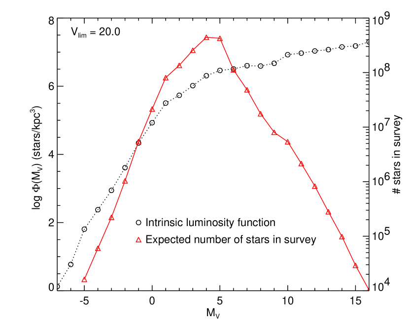
Figure 1: Intrinsic and weighted luminosity functions $\phi_{\mathrm{G}}$ (left vertical scale) and $\psi_{\mathrm{G}}$ (right vertical scale) for our galaxy model. The circles indicate $\phi_{\mathrm{G}}$ and the triangles $\psi_{\mathrm{G}}$, plotted as the actual number of stars expected in the survey.

The Monte Carlo realization of our galaxy model thus proceeds as follows. Given that the luminosity function and spectral type distribution is assumed the same for all Galactic components and positions within the Galaxy, we start by drawing a random value for $M_{V}$ and spectral type from the Hess diagram, weighted in luminosity according to the procedure outlined above. The values for $M_{V}$ are only tabulated as integers which will produce discontinuities in the the generated stellar positions. To avoid this we add a random fraction between 0 and 1 to each generated value of $M_{V}$.

Once the absolute magnitude of a star is chosen, the Von Neumann rejection technique (e.g. Press et al., 1992, Section 7.3) is used to draw a random 3D position within the corresponding magnitude limited sphere. The sum of the densities of each Galactic component, with the appropriate relative amplitudes, is used for this task. Once the position is obtained, the Galactic component to which the star belongs is assigned using the relative amplitude of each component at that position. Finally, a velocity vector is randomly drawn from the kinematical model appropriate for the Galactic component to which the star has been assigned.

We use the Von Neumann rejection technique to generate the positions because the total density distribution is a rather complicated function of the cylindrical coordinates $R$ and $z$ when these are centred on the observer. Although simple to implement, this technique turns out be very inefficient for our case. We want to generate stellar positions within the magnitude limited sphere $\Omega_{V}$ centred on the position of the Sun. To apply the rejection technique we need a function which is everywhere within $\Omega_{V}$ larger than $\rho_{G}$ (see section 7.3 of Press et al., 1992). The simplest function to use is a constant equal to the maximum density within this sphere, however its value cannot be obtained in a simple way. So one is then forced to use the density at the Galactic centre as the upper bound to $\rho_{G}$ and then first generate a position for the star in $\Omega_{V}$ before applying the Von Neumann technique to decide on whether or not to retain the star. For positions far away from the Galactic centre (either faint stars near the Sun or brighter stars far out in the halo) this becomes very inefficient owing to the large density contrast.

To prepare for the volume of data that Gaia will deliver and in order to have a realistic number of Galactic background stars with respect to the satellite stars, we want to achieve a one-to-one sampling of the Gaia survey in our Monte Carlo model of the Galaxy. This implies that we need to generate the positions of $\sim 1.5\times 10^{9}$ stars. This is a task that would take a prohibitive amount of time, even using a fast cluster of Pentium CPUs as we did (see Section 3).

In practice the tracing of satellites on the sky in the parts of the Galactic plane towards the inner Galaxy will be very hard owing mainly to the large extinction in those directions. Therefore we decided not to simulate the part of the sky with Galactic longitude between $-90^{\circ}$ and $+90^{\circ}$, and with Galactic latitude between $-5^{\circ}$ and $+5^{\circ}$. In our Galactic model $\sim 80$ per cent of the stars lie in this region of the sky as seen from the Sun for a survey limited at $V=20$. Hence we now have to simulate ‘only’ $\sim 3\times 10^{8}$ stars. Moreover, cutting out this part of the sky (and thus the Galactic centre) allows us to use a much smaller upper bound for the density which turns out to be the biggest contribution to improving efficiency. Now the entire Monte Carlo Galaxy can be generated in two weeks’ time on a Beowulf computer.

The resulting simulated survey of the Galaxy is thus fully sampled and contains $3.5\times 10^{8}$ stars. For each of these we generated the 6 phase-space coordinates, an absolute magnitude, a population type (bulge, disc or halo) and a spectral type. In Section 4 we discuss in detail how these data were converted into a simulated Gaia survey consisting of positions on the sky, parallaxes, proper motions, radial velocities and photometric information.

Figure 2: Rotation curve for our Milky-Way mass model used in the $N$-body simulations.

3 $N$-body Simulations

In this section we briefly describe the numerical technique used to study the disruption of satellites by the Milky Way’s gravitational potential. Given that our aim is to identify the satellite remnants, we have chosen a rigid potential to represent the Milky Way while self-consistent $N$-body realizations are employed for the satellites.

Table 4: Parameters for our Milky Way mass model used in the $N$-body simulations.

Disc	Bulge	Halo
$M_{\mathrm{d}}=5.6\times 10^{10}\,\mathrm{M}_{\odot}$	$M_{\mathrm{b}}=1.4\times 10^{10}\,\mathrm{M}_{\odot}$	$v_{\mathrm{h}}=186$ kms-1
$R_{\mathrm{d}}=3.5$ kpc	$a=630$ pc	$R_{\mathrm{C}}=12$ kpc
$\beta^{-1}=700$ pc		$q_{\mathrm{\Phi_{h}}}=0.8$

3.1 Numerical models

3.1.1 Galaxy mass model

Our Galaxy mass model for the $N$-body simulations is a composite consisting of a disc, a bulge and a halo. The axisymmetric disc component is represented by the following potential-density pair (Quinn & Goodman 1986):

$$\rho_{\mathrm{d}}(R,z) = {{M_{\mathrm{d}}\beta}\over{4\pi R_{\mathrm{d}}^{2}}}\exp(-R/R_{\mathrm{d}}-\beta|z|)$$ (5)

$$\Phi_{\mathrm{d}}(R,z) = -{{GM_{\mathrm{d}}}\over{R_{\mathrm{d}}^{3}}}\int_{\mathrm{0}}^{\mathrm{\infty}}dk{{k\mathrm{J_{o}}(kR)}\over{(k^{2}+\beta^{2})^{3/2}}}{{\beta^{2}}\over{\beta^{2}-k^{2}}}$$

$$\times[{{\mathrm{e}^{-k|z|}}\over{k}}-{{\mathrm{e}^{-\beta|z|}}\over{\beta}}]$$

where $M_{d}$ is the mass of the disc, $R_{d}$ is the radial scalelength and $\beta^{-1}$ is the vertical scaleheight.

A spherical Hernquist profile has been adopted for the bulge component (Hernquist 1990):

$$\rho_{b}(r)={{M_{b}}\over{2\pi}}{{a}\over{r(r+a)^{3}}}$$ (6)

where $M_{b}$ is the bulge mass and $a$ its scalelength. Another key ingredient of our model is the massive dark halo which is represented by a logarithmic potential (Binney & Tremaine, 1987).

$$\Phi_{\mathrm{h}}=v_{\mathrm{h}}^{2}\ln(R_{\mathrm{C}}^{2}+R^{2}+z^{2}/q_{\mathrm{\Phi_{h}}}^{2})$$ (7)

where $v_{\mathrm{h}}$, $R_{\mathrm{C}}$ and $q_{\mathrm{\Phi_{h}}}\equiv(c/a)_{\mathrm{\Phi_{h}}}$ are constants. The last parameter is the flattening of the halo potential. Table 4 summarises the parameters of our Milky Way mass model and its rotation curve is shown in Figure 2. The total mass of the Milky Way model, truncated at 200 kpc, is $1.7\times 10^{12}$ M_⊙.

Table 5: Self-consistent satellite models ($10^{6}$ particles).

	S1	S2
$M_{\mathrm{s}}$	$5.6\times 10^{7}\,\mathrm{M}_{\odot}$	$2.8\times 10^{7}\,\mathrm{M}_{\odot}$
$r_{\mathrm{t}}$	$3150$ pc	$3150$ pc
$c$	$0.9$	$0.9$

Current models of large scale structure and galaxy formation postulate that small objects are the first to form and then aggregate into larger systems (e.g. Kauffmann & White, 1993). In the non-baryonic CDM model, this hierarchical assembly of haloes leads to triaxial shapes with average axis ratios of $(c/a)_{\mathrm{\rho_{h}}}=0.5$ and $(b/a)_{\mathrm{\rho_{h}}}=0.7$ (Dubinski & Carlberg, 1991). But, when a dissipative gas component is incorporated they tend to be oblate with axis ratios of $(c/a)_{\mathrm{\rho_{h}}}=0.5$ and $(b/a)_{\mathrm{\rho_{h}}}>0.7$ (Dubinski, 1994). Furthermore, haloes formed within a $\Lambda$CDM model are more spherical with an axis ratio of $(c/a)_{\mathrm{\rho_{h}}}\simeq 0.71$ while rounder haloes with $(c/a)_{\mathrm{\rho_{h}}}\simeq 0.77$ are obtained for a $\Lambda$WDM model (Bullock, 2002). The shape of our galaxy’s halo is disputed and in this respect the disruption of the Sagittarius dwarf galaxy provides a useful test case. By studying tidal tails from this dwarf galaxy Ibata et al. (2001) ruled out the possibility that the halo is significantly oblate (i.e. with an axis ratio of $q_{\mathrm{\rho_{h}}}<0.7$). However, Martínez-Delgado et al. (2004) suggest that the potential of the Milky Way dark halo, as constrained by observations of the Sagittarius dwarf, is likely to be oblate with $q_{\mathrm{\Phi_{h}}}=0.85$, while modelling of radial velocities of M-giants in the Sagittarius dwarf by Helmi (2004) suggests that the halo is prolate with an average density axis ratio within the orbit of Sagittarius close to $5/3$. Given all this evidence supporting a non-spherical halo, we have adopted an oblate one to carry out our numerical simulations with an axis ratio of $q_{\mathrm{\Phi_{h}}}=(c/a)_{\mathrm{\Phi_{h}}}=0.8$ which corresponds to a flattening in density of $q_{\mathrm{\rho_{h}}}\approx 0.73$ and $q_{\mathrm{\rho_{h}}}\approx 0.42$ in the inner and outer regions, respectively.

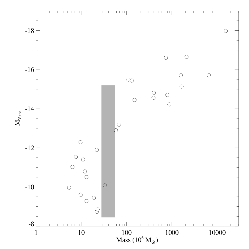
Figure 3: Luminosity versus mass for dwarf galaxies of the Local Group (open circles). The data were taken from Mateo (1998) and the luminosities were converted to total $V$-band magnitudes according to $M_{V,\mathrm{tot}}=-2.5\log L_{V,\mathrm{tot}}+4.8$. The shaded region shows the mass range of our $N$-body systems (masses of $2.8\times 10^{7}$ and $5.6\times 10^{7}$ M_⊙) and the corresponding possible luminosity range. The luminosity of a satellite of a given mass will depend on its mass function and mass to light ratio.

3.1.2 Satellite mass models

Positions and velocities for particles in our self-consistent satellite models are randomly drawn from King models (King 1966). The latter are a series of truncated isothermal spheres parametrized by a concentration defined as $c=\log(r_{\mathrm{t}}/r_{\mathrm{c}})$ where $r_{\mathrm{t}}$ and $r_{\mathrm{c}}$ are the tidal and core radii, respectively. These models quite well fit the dwarf spheroidal galaxies (Vader & Chaboyer 1994). To completely define a satellite we have to specify its mass and tidal radius in addition to its concentration (see Table 5). In all cases, each satellite consists of $10^{6}$ equal-mass particles.

Figure 3 shows the luminosity and mass distribution of real Local Group dwarf galaxies. The masses and luminosities ($V$-band) vary between $\sim 10^{7}$ and $\sim 10^{10}$ M_⊙, and $\sim 3\times 10^{5}$ and $\sim 10^{9}$ L_⊙, respectively (see Mateo, 1998). This means that our simulated dwarf galaxies fall in the low-mass end of the satellite mass distribution. The grey shaded area in Fig. 3 shows the range of possible luminosities (given the observational data) for systems with masses between $2.8\times 10^{7}$ and $5.6\times 10^{7}$ M_⊙. The range of possible luminosities for our simulated dwarf galaxies is important for the discussion in Section 4.3.

Table 6: Orbital parameters for our experiments.

Run	Satellite	Pericentre	Apocentre	Inclination
	Model	(kpc)	(kpc)	Angle
1	S1	$8.75$ kpc	$105$ kpc	$30^{o}$
2	S1	$7$ kpc	$60$ kpc	$45^{o}$
3	S2	$7$ kpc	$80$ kpc	$60^{o}$
4	S2	$40$ kpc	$60$ kpc	$25^{o}$
5	S2	$3.5$ kpc	$55$ kpc	$45^{o}$

Figure 4: Satellite orbits (see Table 6) projected onto the principal axes of our Milky Way galaxy model. The Galactic disc corresponds to the $XY$ projection. Distances are in kpc.

3.2 Numerical tools

The simulations were evolved with a parallel tree-code for about $10$ Gyr. It uses a tolerance parameter of $\theta=0.75$ and a fixed integration time-step of $1.3$ Myr (Dubinski, 1996). Forces between particles are computed including the quadrupole terms and the gravitational potential uses a Plummer softening length of $35$ pc. With these parameters the energy conservation in all cases was better than $0.1$%. All our numerical runs were performed on a Beouwulf computer at the IAUNAM-Ensenada. It has $32$ Pentium processors running at 450 MHz (Velázquez & Aguilar, 2003). Each simulation took 96 hours of ‘wall-clock’ time.

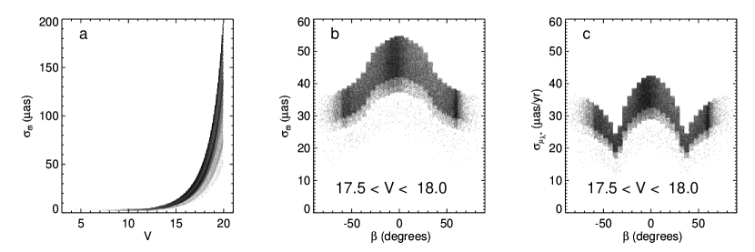
Figure 5: The distribution of errors in the simulated Gaia astrometric parameters for 1 million stars from the model Galaxy. The grey scale indicates the number of stars. Panel (a) shows the parallax errors as a function of $V$, the spread is caused by the colour dependence of the errors (see Appendix A). Panel (b) shows the variation of the parallax errors with ecliptic latitude $\beta$ and panel (c) shows the dependence of the errors in $\mu_{\lambda*}$ on $\beta$. In order to clearly bring out the variation over the sky, the magnitude range of the stars was restricted for panels (b) and (c). The discrete steps in (b) and (c) are caused by the discrete tabulation of the dependence of the errors on $\beta$. There is no dependence of the errors on ecliptic longitude and $\sigma_{\mu_{\beta}}$ shows practically no variation with $\beta$.

3.3 Numerical experiments

A total of five orbits were chosen to follow up the disruption of the satellite models. The parameters that define them are listed in Table 6. The last column refers to the initial inclination angle of the orbit with respect to the plane of the Galactic disc. Notice that most of these orbits have a pericentre radius inside the Solar radius. Figure 4 shows the different projections of these orbits onto the main axes of our Milky Way mass model where the plane of the Galactic disc corresponds to the $XY$ projection. Since the Milky Way galaxy is represented by a rigid potential and dynamical friction is ignored, the orbital decay of the satellite is not taken into account.

4 Modelling the Gaia Survey

In this section we describe how the stellar positions and velocities from the Monte Carlo model of the Galaxy and the $N$-body models of the satellites are converted to the data that Gaia will deliver: sky-positions; parallaxes; proper motions; and radial velocities. We also describe how to put together the Galaxy and satellite simulations taking care to correctly account for the variation of the number of visible stars along the orbit of the satellite, while using as much of the $N$-body particles as possible.

4.1 The Galactic data

To convert phase-space coordinates in the Galaxy model to Gaia data we first translate them to the barycentric coordinate frame, which has the same axes as the Galactocentric system used for the simulations but with its origin at the Sun’s position and velocity. The barycentric position $\mathbf{r}^{\mathrm{b}}=\mathbf{r}-\mathbf{r}_{\odot}$ and velocity $\mathbf{v}^{\mathrm{b}}=\mathbf{v}-\mathbf{v}_{\odot}$ are converted to the five astrometric parameters and the radial velocity $v_{\mathrm{rad}}$. The astrometric observables are the Galactic coordinates $(\ell,b)$, the parallax $\varpi$, and the proper motions $\mu_{\ell*}=\mu_{\ell}\cos b$ and $\mu_{b}$. The units of parallax and proper motion are micro-arcsecond ($\mu$as) and $\mu$as yr^-1. The radial velocity is given in km s^-1.

Subsequently the expected Gaia errors are added to the observables according to the accuracy assessment described in Chapt. 8 of the Gaia Concept and Technology Study Report (ESA, 2000). The dominant variation of the size of the errors is with the apparent brightness of the stars in addition to which there is a dependence on colour and position on the sky. Thus, as a first step we calculate the $V$-band magnitude of each star from its parallax and assign a $(V-I)$ colour based on the spectral type of the star. The relation between spectral type and $(V-I)$ was taken from Cox (2000). Note that no extinction is included in our model Galaxy.

Like Hipparcos (see ESA, 1997) Gaia will be a continuously scanning spacecraft and will accurately measure one-dimensional coordinates along great circles in two fields of view simultaneously, separated by a well-known angle. The accuracy of the astrometric measurements will thus depend on how the parallactic plus proper motions of a particular object project onto these great circles. Because Gaia will collect its measurements from an orbit in the plane of the Ecliptic the astrometric errors will vary over the sky as a function of the Ecliptic latitude $\beta$. For the positions and proper motions the latter variation of the precision is caused mainly by the variation in the number of times an object is observed by Gaia, which is dependent on the details of the way Gaia scans the sky over the mission lifetime. For the parallax measurements the dominant factor is the decrease in measurement precision from the ecliptic pole to the equator owing to the way the parallax ellipse of a star projects onto a great circle scan (the parallax factor). The precision of the radial velocity measurements varies as a function of $V$ and spectral type but is assumed not vary over the sky in our simulations.

The dependence of the errors on the Ecliptic coordinates $(\lambda,\beta)$ of a star is taken into account in the simulations by rotating the astrometric data to Ecliptic coordinates, adding the errors and rotating the result back to the Galactic reference frame. As a consequence correlations will be introduced between the errors in $\ell$ and $b$ as well as $\mu_{\ell*}$ and $\mu_{b}$, even in the absence of any correlation in the Ecliptic reference frame.

Figure 5 illustrates the dependence of the errors in the astrometric data on the apparent brightness of the star and its position on the sky. The variation with stellar magnitude is the strongest. We show only the variation of parallax error $\sigma_{\varpi}$ with $V$ as the variation is similar for the other astrometric parameters. The spread in $\sigma_{\varpi}$ at each value of $V$ is caused by the colour dependence of the astrometric errors (smaller errors for redder stars, see Appendix A). The variation of the errors over the sky is shown in Ecliptic coordinates $(\lambda,\beta)$ and is prominent only for $\sigma_{\varpi}$ and $\sigma_{\mu_{\lambda*}}$. The errors only vary as a function of ecliptic latitude $\beta$. Finally we point out that the relative error in the sky positions is at most $\sim 10^{-9}$ (which is 200 $\mu$as expressed in radians) meaning that distance errors perpendicular to the line of sight to even the most distant stars (at about 100 kpc) amount to no more than about $10^{-4}$ pc. Hence we will ignore errors on the sky positions in the rest of the paper.

Finally, the steps taken to construct the simulated Gaia catalogue are summarized here:

1. From $\mathbf{r}$ and $\mathbf{v}$ calculate the barycentric position and velocity.

2. Transform these to the astrometric parameters in the Galactic coordinate system and the radial velocity.

3. Calculate $V$ from $M_{V}$ and $\varpi$.

4. Find the $(V-I)$ colour corresponding to the spectral type of the star.

5. Rotate the astrometric parameters to the Ecliptic coordinate system.

6. Add the astrometric errors as a function of $V$, $(V-I)$ and Ecliptic latitude.

7. Rotate the resulting astrometric parameters back to the Galactic coordinate system.

8. Add radial velocity errors.

For details please see Appendix A.

4.2 The satellite data

Given $V$ and $(V-I)$, the satellite stars are treated in exactly the same way as the stars in the Monte Carlo Galaxy where the calculation of the astrometric and radial velocity data is concerned. Hence here we describe only how the absolute magnitudes and colours of the satellite stars are chosen.

We assume our simulated satellites represent disrupted dwarf galaxies and in this and the following sub-section we will make a distinction between real dwarf galaxies and our simulated $N$-body satellites. We will refer to the former as ‘dwarf galaxies’ or ‘satellites’ and to the latter as ‘$N$-body systems’ or ‘simulated satellites’.

All $N$-body systems are assumed to represent a single stellar population of a certain age and metallicity, which forms a single isochrone in a colour-magnitude diagram. Combining this isochrone with a mass function $\xi(m)$ for the satellite stars, we assign to each $N$-body particle a value for $M_{V}$ and $(V-I)$. We use the isochrones by Girardi et al. (2000). These isochrones have been transformed to several different photometric systems as described in Girardi et al. (2002). The procedure for a particular star is to first generate its mass and then to interpolate the isochrone in mass to find the corresponding values of $M_{V}$ and $(V-I)$.

The colour-magnitude diagrams for a number of Local Group dwarf galaxies are very similar to those of Galactic globular clusters (see e.g., Feltzing, Gilmore & Wise, 1999; Monkiewicz et al., 1999). This suggests that we can use a globular cluster like mass function for our $N$-body systems. Based on the study of a dozen globular clusters Paresce & De Marchi (2000) propose a lognormal mass function for these systems for stars below about 1 M_⊙. This mass function has a characteristic mass of $0.33$ M_⊙ and a standard deviation of $0.34$. The slope of the mass function between $\sim 0.3$ and $\sim 1$ M_⊙ is similar to that of a power-law mass function for which $\xi(m)\propto m^{-\alpha}$, with $\alpha\approx 1.5$. For N-body snapshots older than 5 Gyr the stars in the simulated satellites will all have masses less than about 2 M_⊙ and for simplicity we use a single power-law mass function $\xi(m)\propto m^{-1.5}$. Hence we may be overestimating the number of low-mass stars (below $0.3$ M_⊙) in our $N$-body systems with respect to the more massive stars.

4.3 Converting satellite $N$-body particles to stars

Having made a considerable effort to realistically — in terms of the number of stars — simulate the Galaxy as it will be seen by Gaia, we want to ensure that the satellite $N$-body particles are properly converted to simulated stars representing a dwarf galaxy. Getting this right is not trivial and we explain below why this is the case and describe in detail our solution to this problem.

Given a certain distribution of stars along the orbit of a particular dwarf galaxy (corresponding to an $N$-body ‘snap-shot’), the number of stars from this satellite that will end up in the Gaia catalogue depends on three factors:

1. The overall number of stars (i.e., luminous particles) in the dwarf galaxy. This number is determined by its overall luminosity and the stellar mass function.

2. The Gaia survey limit. This magnitude limit determines the faintest dwarf galaxy stars visible by Gaia.

3. The variation of the number of visible satellite stars along the orbit. This variation is caused by the variation in distance from the dwarf galaxy stars to the Sun.

If we take the $N$-body particles as representing a sampling of the distribution of the real satellite stars along the orbit, then the expected number of satellite stars visible in the Gaia survey can be calculated as follows. The overall number of stars (luminous particles) $N_{\mathrm{lum}}$ in a real dwarf galaxy can be obtained from its total luminosity in the $V$-band $L_{V,\mathrm{tot}}$ and its mass function $\xi(m)$:

$$N_{\mathrm{lum}}=\frac{L_{V,\mathrm{tot}}}{\langle L_{V}\rangle}\,,\quad\langle L_{V}\rangle=\frac{\int L_{V}(m)\xi(m)dm}{\int\xi(m)dm}\,.$$ (8)

$L_{V}(m)$ is the $V$-band luminosity of a dwarf galaxy star with mass $m$ and $\langle L_{V}\rangle$ is the average stellar luminosity in the dwarf galaxy. At each distance $s_{i}$ at which an $N$-body particle is located, the fraction of visible satellite stars is set by the magnitude limit $M_{V,\mathrm{max}}$ which is given by:

$$M_{V,\mathrm{max}}(s_{i})=V_{\mathrm{lim}}-5\log s_{i}+5\,,$$ (9)

where $V_{\mathrm{lim}}$ is the Gaia survey limit. The fraction of visible satellite stars $f_{i}$ at distance $s_{i}$ is then:

$$f_{i}(s_{i})=\frac{\int_{m(M_{V,\mathrm{max}})}^{m_{\mathrm{up}}}\xi(m)dm}{\int\xi(m)dm}\,,$$ (10)

where $m_{\mathrm{up}}$ is the upper mass limit of the mass function. The overall fraction $f$ of visible satellite stars is then given by:

$$f=\frac{\sum_{i}f_{i}(s_{i})}{N_{\mathrm{sim}}}\,,$$ (11)

where $N_{\mathrm{sim}}$ is now the total number of simulated satellite particles. Hence the number of satellite stars expected in the Gaia survey is $fN_{\mathrm{lum}}$. Note that we assume that the mass function does not vary along the orbit of the satellite. This may not be realistic if the satellite preferentially looses lower mass stars owing to tidal forces.

Now, for a normal mass function the number of low-mass stars will heavily dominate, which means that the fractions $f_{i}$ can be very small depending on the distance $s_{i}$. Figure 6 shows an example of this for a snapshot at about 10 Gyr of $N$-body run no. 1 (see Table 6). The stellar population of the simulated satellite is represented by a 10 Gyr isochrone for a metallicity $Z=0.004$, with a mass function $\xi(m)\propto m^{-1.5}$. Three things are shown as a function of the distance $s_{i}$ of each $N$-body particle $i$. The shaded histogram shows the distribution of distances $s_{i}$ and illustrates the wide variety of distances at which the simulated satellite particles are located. The solid line shows for each distance $s_{i}$ the fraction of visible stars $f_{i}$ calculated as outlined above. The $N$-body particles are taken to represent a fully populated mass function which in this case ranges between $0.15$ and $0.88$ M_⊙. Note that $f_{i}$ is nowhere larger than $\sim 0.1$, while the overall fraction $f$ of visible stars is $2.5\times 10^{-3}$. This means that if we assume that our $N$-body particles represent stars over the full range of the satellite mass function, only $2\,500$ out of the 1 million simulated stars will end up in our synthetic Gaia catalogue!

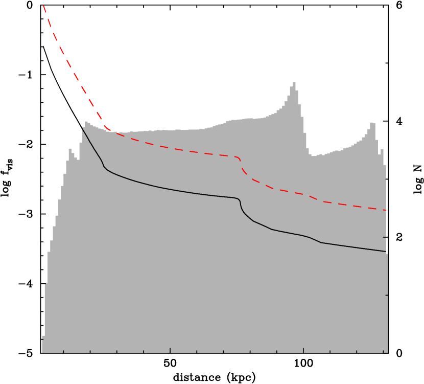
Figure 6: Visible fraction of the simulated satellite stars at each $N$-body particle position as a function of the distance to the observer for $N$-body run no. 1. The shaded histogram (vertical scale on the right) shows the distribution of distances $s_{i}$. The solid line (vertical scale on the left) shows for each distance $s_{i}$ the fraction of visible stars $f_{i}$ calculated as in Section 4.3. The features in this line reflect features in the luminosity function. The dashed line shows the fraction of visible stars when taking into account only the stars brighter than the faintest satellite star that enters the Gaia survey. The fractions of visible stars were calculated using a 10 Gyr isochrone of metallicity $Z=0.004$ and a mass function $\xi(m)\propto m^{-1.5}$. The overall fraction of visible $N$-body particles is only $2.5\times 10^{-3}$ and $10^{-2}$ for the two cases considered.

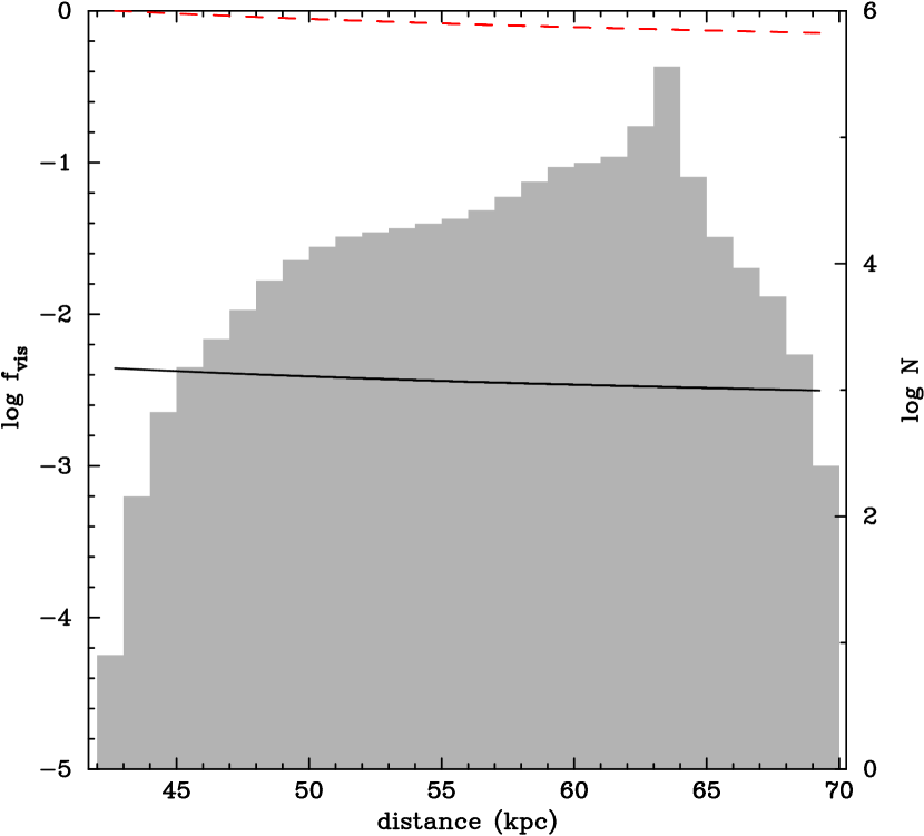
Figure 7: Same as Fig. 6 for the simulated satellite from $N$-body run no. 4. A 5 Gyr isochrone and the same mass function were used. Note the much smaller range in distances for this $N$-body system, resulting in a much larger fraction of visible stars if the luminosity function is cut off at $M_{V}\leq M_{V,\mathrm{faintest}}$. The overall fraction of visible stars is $3.4\times 10^{-3}$ when using the full mass function and $0.78$ when only stars with $M_{V}\leq M_{V,\mathrm{faintest}}$ are considered.

This is clearly a very wasteful way to make use of the (computationally) expensive $N$-body calculations and the question is how to retain more $N$-body particles in the synthetic Gaia catalogue whilst at the same time preserving the variation of the visible fraction of stars along the $N$-body system’s orbit. One straightforward improvement can be made by realizing that for mass functions that extend all the way to late M-dwarfs most of the generated synthetic satellite stars are too faint to ever make it into the Gaia survey, regardless of the position at which they are located along the satellite orbit. To eliminate this problem we can first find the position in the $N$-body snapshot that is closest to the Sun (at a distance $s_{\mathrm{min}}$) and calculate the corresponding absolute magnitude, $M_{V,\mathrm{faintest}}$, of the faintest satellite stars visible by Gaia. Subsequently in assigning luminosities to the simulated satellite stars we use the luminosity function only for $M_{V}\leq M_{V,\mathrm{faintest}}$. The result is shown in Fig. 6 by the dashed line. The visible fraction of stars increases everywhere by more than an order of magnitude due to the exclusion of the faintest (never visible) stars. However the overall fraction of visible stars is still very low at $9.8\times 10^{-3}$. This is a consequence of the large variation in distances for the orbit of the simulated satellite from $N$-body run no. 1. Figure 7 shows the distribution of distances and values of $f_{i}$ for the satellite from run no. 4 at 5 Gyr (using a 5 Gyr isochrone and the same mass function), which has a much more circular orbit with much less distance variation (compare the orbits in Fig. 4). For this $N$-body system one can retain about 78 per cent of the $N$-body particles if the luminosity function cut-off at $M_{V}\leq M_{V,\mathrm{faintest}}$ is used.

A further improvement is now obvious. Instead of cutting off the luminosity function at $M_{V,\mathrm{faintest}}$ we choose a brighter limit and retain more of the $N$-body particles in the synthetic Gaia catalogue. This can be interpreted as simulating the fact that in practice one will use bright ‘tracer’ stars (such as those at the tip of the AGB or RGB) to map out the satellite in phase-space. That is, we assume that the $N$-body particles only represent stars at the high mass end of the satellite’s mass function. In fact most of the present surveys for substructure in the Galactic halo rely on using tracer populations that are more easily isolated photometrically in colour-magnitude diagrams (see e.g., Majewski et al., 2003; Martin et al., 2004; Rocha-Pinto et al., 2004; Helmi, 2004).

In principle the luminosity function cut-off magnitude $M_{V,\mathrm{tracer}}$ can be chosen bright enough to retain all $N$-body particles. However, there are two constraints on its value, the first of which is the obvious limit set by the magnitude of the brightest star in the luminosity function. The second constraint is set by the desire for a realistic simulation of a satellite as it will appear in the Gaia catalogue. By assuming that the $N$-body particles represent only a tracer population we are effectively simulating a more massive dwarf galaxy when converting the $N$-body results to Gaia observations. In reality we have simulated rather small dwarf galaxies (see Fig. 3) which cannot be scaled up trivially to more massive systems because the latter respond differently to the Galactic tidal forces. Thus a balancing between the number of retained $N$-body particles and the total mass (or luminosity) of a real dwarf galaxy that we wish to simulate is required.

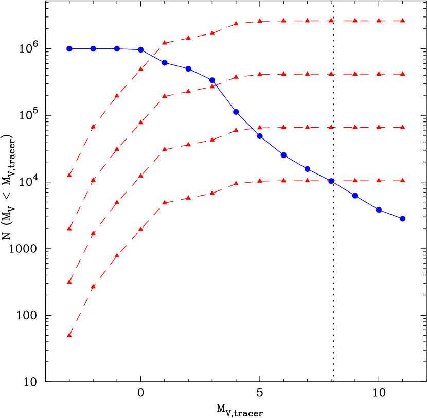
Figure 8: Visible number of stars as a function of the luminosity function cut-off $M_{V,\mathrm{tracer}}$ for a satellite with its stars distributed along the orbit of $N$-body run no. 1. The dashed curves with triangles show the numbers for ‘real’ dwarf galaxies (i.e., with fully populated luminosity functions) of total luminosities: $M_{V,\mathrm{tot}}=-17,-15,-13,-11$ (where $M_{V,\mathrm{tot}}=-2.5\log L_{V,\mathrm{tot}}+4.8$). The dotted line shows the value of $M_{V,\mathrm{faintest}}$ beyond which the dashed curves become flat. The solid curve with dots shows the numbers of visible stars for the $N$-body system, where now all stars are assumed to be brighter than $M_{V,\mathrm{tracer}}$. The fractions of visible stars were calculated using a 10 Gyr isochrone of metallicity $Z=0.004$ and a mass function $\xi(m)\propto m^{-1.5}$.

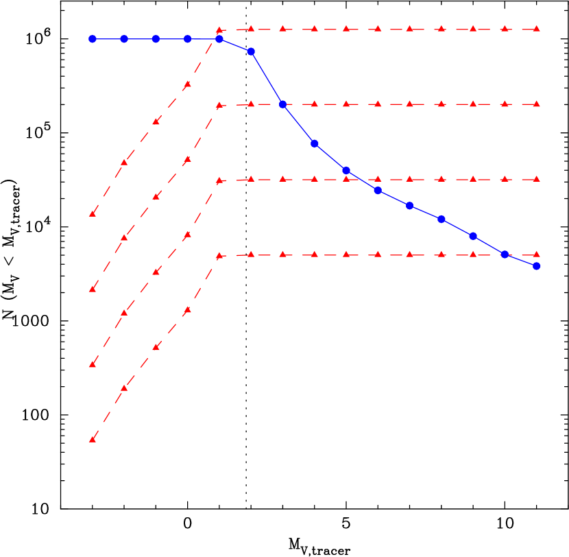
Figure 9: Same as Fig. 8 for a satellite with its stars distributed along the orbit of from $N$-body run no. 4. A 5 Gyr isochrone and the same mass function were used. Note the brighter value of $M_{V,\mathrm{faintest}}$ which reflects the larger average distance of this satellite.

This balancing is illustrated in Figs. 8 and 9 for the $N$-body systems discussed above. The figures show for the $N$-body system and for the corresponding real dwarf galaxies how the number of stars visible by Gaia changes as the magnitude cut-off of the luminosity function, $M_{V,\mathrm{tracer}}$, changes. These numbers are calculated according to equations (8)–(11). For a real dwarf galaxy the number of visible stars will increase as the value of $M_{V,\mathrm{tracer}}$ goes up, reflecting a probing of the luminosity function to fainter magnitudes. At some point $M_{V,\mathrm{tracer}}$ becomes larger than $M_{V,\mathrm{faintest}}$ and the number of visible stars stays constant (probing deeper into the luminosity function only adds stars invisible to Gaia). This is shown by the dashed curves and triangles, where each curve represents a dwarf galaxy of different $L_{V,\mathrm{tot}}$ (or total mass). The dotted line shows the value of $M_{V,\mathrm{faintest}}$ beyond which the curves are flat.

For the $N$-body system the number of visible particles will decrease as the value of $M_{V,\mathrm{tracer}}$ goes up. This is because now all particles are assumed to be brighter than $M_{V,\mathrm{tracer}}$ which leads to a larger fraction of simulated stars that are fainter than the survey limit as the luminosity function cut-off becomes fainter. In Figs. 8 and 9 the solid curve with dots represents the visible number of stars for the $N$-body system. Note that this curve continues to drop beyond $M_{V,\mathrm{tracer}}=M_{V,\mathrm{faintest}}$ which reflects the increasing number of simulated stars that will never enter the Gaia survey.

The balancing of the number of retained $N$-body particles and the total mass of the dwarf galaxy we wish to simulate thus consists of choosing a dwarf galaxy luminosity and then finding the value of $M_{V,\mathrm{tracer}}$ for which the number of expected tracer stars from this satellite in the Gaia survey is equal to the number of retained $N$-body particles. For $N$-body run no. 1 one can simulate an $M_{V,\mathrm{tot}}=-17$ satellite by choosing $M_{V,\mathrm{tracer}}\approx 0.5$, which then results in between $7\times 10^{5}$ and $8\times 10^{5}$ $N$-body particles entering the synthetic Gaia catalogue. Note that in practice one can choose a value of $M_{V,\mathrm{tracer}}$ corresponding to an approximate value of $M_{V,\mathrm{tot}}$ by inspecting diagrams such as Figs. 8 and 9, and then calculate the actual value of $M_{V,\mathrm{tot}}$ based on the amount of $N$-body (tracer) particles that enter the simulated Gaia survey.

We now return to Fig. 3 which shows that for the mass range of the satellites we have simulated the total $V$-band magnitude can be at most $M_{V,\mathrm{tot}}\approx-15$. From Figs. 8 and 9 one can see that this luminosity is simulated for $M_{V,\mathrm{tracer}}\approx 3$ and that then we retain about $2\times 10^{5}$ $N$-body particles for each satellite. We still consider this wasteful and decided to use $M_{V,\mathrm{tracer}}=0.5$ in order to retain many more $N$-body particles. This implies an unrealistic value of $M_{V}\approx-17$ for the absolute magnitude of the simulated satellites in the $V$-band. The main problem being that the corresponding masses of more than $10^{9}$ M_⊙ (see Fig. 3) would require simulations with at least an order of magnitude more particles and with the effects of dynamical friction included. This was beyond our computational capabilities at the time the simulations were done. However, the purpose of this paper is not to provide detailed and completely realistic simulations of the Galaxy and its satellites. The main purpose is to get an insight into the challenges one will have to deal with when searching for the debris of past merger events in the Gaia data. Therefore we feel it is more important to get a good sampling of the distribution of satellite stars in the Gaia catalogue, by artificially increasing their numbers, than to construct a completely realistic simulation of the satellite debris.

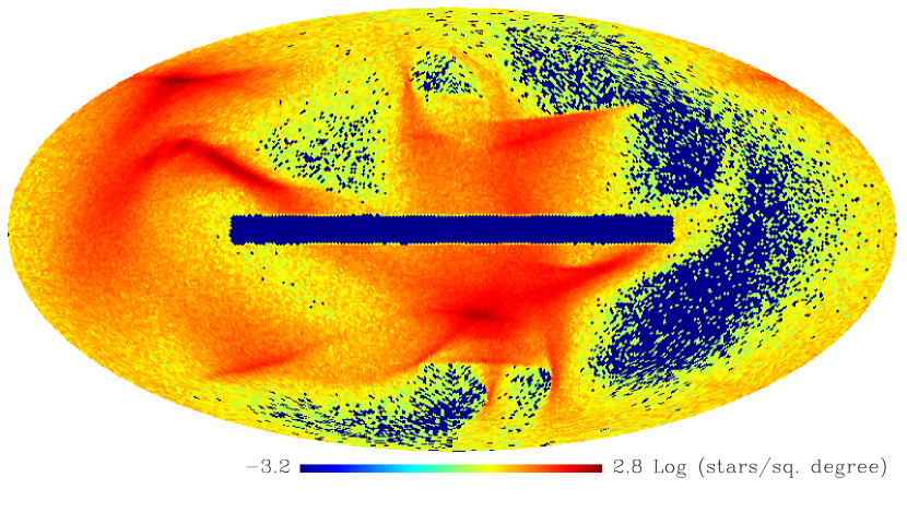
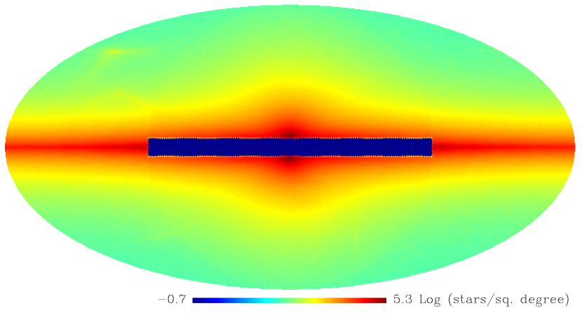
Figure 10: Mollweide projections of the distribution on the sky of the stars in our simulated Gaia catalogue. The top image shows only the satellites projected on the sky (from simulation runs no. 1 and 5 at 10 Gyr, where an extra satellite was generated by reversing the angular momentum for run 1). The bottom image shows the Galaxy and satellite stars combined. Note how the satellite stars become almost totally invisible. The only conspicuous over-density is in the top left corner of the image. The dark rectangle is the area on the sky with coordinates $-90^{\circ}\leq\ell\leq+90^{\circ}$ and $-5^{\circ}\leq b\leq+5^{\circ}$ that was left out of the simulations. The figures were generated using the Healpix (Gorski, Hivon & Wandelt, 1999) division of the celestial sphere into cells of equal area and counting the stars inside each cell. Dark areas correspond to empty cells while the individual dots indicate cells with 1 or more stars. Areas where all contiguous cells are filled appear as a grey scale.

Finally, we summarise here the steps for simulating the satellite galaxy as it will appear in the Gaia catalogue:

1. calculate the distance to each $N$-body particle.

2. Choose a value $M_{V,\mathrm{tracer}}$ for the minimum brightness of the tracer stars represented by the $N$-body particles.

3. Re-normalise the luminosity function between $M_{V}(m_{\mathrm{up}})$ and $M_{V,\mathrm{tracer}}$ (i.e., all $N$-body particles represent stars brighter than $M_{V,\mathrm{tracer}}$).

4. Generate simulated stars for each $N$-body particle position (distance) according to the renormalized luminosity function and decided whether or not they are bright enough to enter the Gaia survey.

5. For stars bright enough to enter the Gaia survey assign a $(V-I)$ colour by interpolating in mass along the isochrone.

6. Generate the Gaia data according to the steps outlined in Section 4.1.

This procedure ensures a properly sampled luminosity function along the orbit of the dwarf galaxy.

Our procedure assumes that one can select the bright tracer stars a priori which may not always be possible in practice and may not be desirable. A way to get around this problem and still use as many $N$-body particles as possible is the following. Assume that all $N$-body particles are brighter than $M_{V,\mathrm{faintest}}$ and calculate the predicted number of $N$-body particles that make it into the survey as for Figs. 8 and 9. Calculate the ratio $R=N_{\mathrm{sim}}/N_{\mathrm{vis}}$, where $N_{\mathrm{vis}}$ is the number of visible particles for $M_{V,\mathrm{tracer}}=M_{V,\mathrm{faintest}}$. Subsequently repeat steps (1)–(6) above $R$ times for each $N$-body particle. That is, generate $R$ stars for each $N$-body particle and retain those that are bright enough to enter the survey. This way all $10^{6}$ $N$-body particles can be retained in the simulated Gaia data whilst still retaining a proper luminosity function sampling along the orbit of the dwarf galaxy. However one then faces the problem of possibly having simulated a system that is too massive (but this can be tuned by not retaining all $10^{6}$ particles) and of having simulated $R$ stars at exactly the same position with the same velocity vector. It is not clear how one would redistribute these extra stars along the dwarf galaxy orbit such that their energy and angular momentum are consistent with that of the $N$-body particles. We therefore decided not to pursue this option further.

To close this section we show in Fig. 10 the sky distribution of the stars in our simulated Gaia catalogue. The simulated satellites included in these figures correspond to $N$-body runs 1 and 5 of Table 6 where a third satellite was generated by reversing the angular momentum of the satellite from run 1. The main thing to note is how the satellite stars are completely swamped by the Galactic stars in these sky projections. This is not a new fact but serves to illustrate the need for clever search techniques to find the debris of disrupted satellites, an issue to which we turn in the next section.

5 Results from Gaia Survey Modelling

Helmi & White (1999) showed that it will be quite difficult to find spatial correlations in the debris originating from satellites, whose disruption occurred in the early evolution of the Milky Way after several passages through pericentre. In this respect, techniques to identify streamers like the ‘Great Circle Cell Counts’ proposed by Johnston et al. (1996) will be of little practical use. This method requires that the orbital plane of the satellite remains almost unchanged during its disruption process, so that the debris occupies great circles on the sky as seen from the Galactic Centre. This only occurs if the outer halo is spherical or if the satellite follows a polar or planar orbit in the case of an oblate halo.

Helmi et al. (1999) showed that useful information can be obtained from the phase-space structure of these fossil remnants which allows tracing the merger history of our Galaxy. Initially satellites are clumped in both the configuration and velocity space, and also in the integrals of motion space. The method of searching for debris in the integrals of motion space relies on the basic assumption that these quantities are conserved, or evolve only slightly, and hence their lumpiness should be preserved. For a spherically symmetric halo the integrals of motions are the energy, total angular momentum and angular momentum around the Galactic $Z$-axis, $(E,L,L_{z})$; for an axisymmetric halo $E$ and $L_{z}$ are preserved while $L$ evolves owing to the orbital precessing of the satellite but it still exhibits some degree of coherence. The integrals of motion technique was applied by Helmi & de Zeeuw (2000) to an artificial Gaia halo catalogue generated from $N$-body simulations of the disruption of satellites in a Galactic potential. From this study, they conclude that identifying substructure within the stellar halo resulting from merger events in the past will be relatively easy even after Gaia observational uncertainties are taken into account.

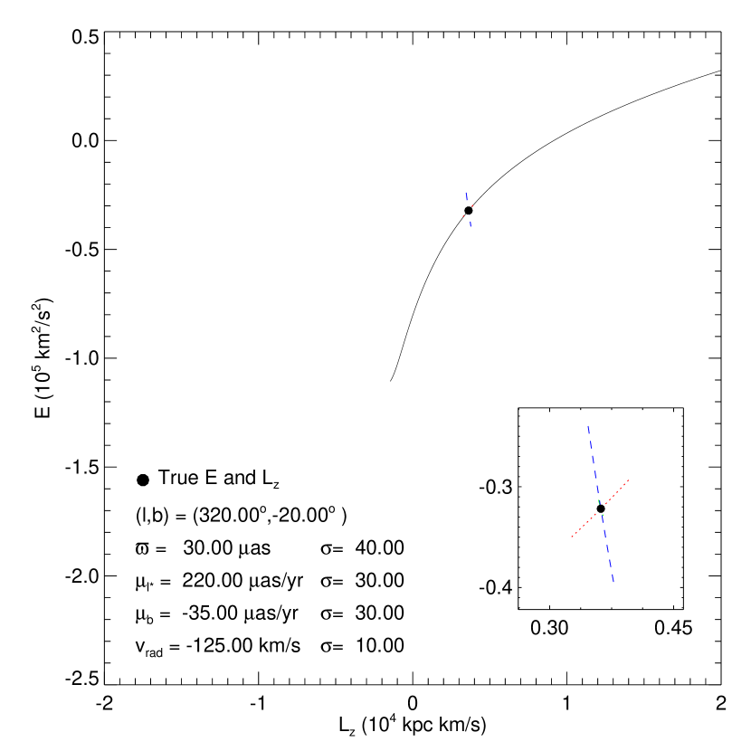
Figure 11: Error propagation in the $E$–$L_{z}$ plane. The effect of the astrometric and radial velocity errors on the observed value of $E$ and $L_{z}$ is shown using the example of a particular star with $\mathbf{r}$ and $\mathbf{v}$ corresponding to the satellite from simulation run 1 at 10 Gyr. Each line indicates how $E$ and $L_{z}$ change from the true value (indicated by the dot) as the observables are varied within $\pm 3\sigma$ from their true values. The values of the astrometric parameters, the radial velocity and the corresponding errors are listed in the legend. The solid line shows the effect of the error in the parallax. The dotted line shows the effect of errors in $\mu_{\ell*}$. The dashed line indicates the effect of radial velocity errors. The inset enlarges the region around the true value of $(E,L_{z})$ in order to better show the effects of the proper motion and radial velocity errors. Note that the error in $\mu_{b}$ has almost no effect on $(E,L_{z})$ for this particular star. The scale of the figure is the same as for Fig. 12. For convenience the potential energy was computed using the potential from equations (8)–(10) in Helmi & de Zeeuw (2000).

However Helmi & de Zeeuw (2000) made two important simplifying assumptions. They constructed a synthetic Gaia catalogue consisting of stars that are intrinsically as well as apparently bright ($M_{V}=1$, $V\leq 15$), and which are all located relatively near the Sun ($d<6$ kpc). The limit on apparent brightness was set by the demand of having good radial velocities available for their sample. Secondly, their simulated halo consists exclusively of in-falling satellite Galaxies. These two assumptions lead to a sample of halo stars which have small observational errors and will be highly clumped in the integrals of motion space, making the disentangling of the different debris streams relatively easy.

In reality there may well be a ‘background’ population of halo stars that have a smooth distribution in $(E,L,L_{z})$ space owing to previous phase mixing and dynamical friction or because they constitute a component that was formed in a monolithic collapse and thoroughly mixed by violent relaxation. In addition real debris streams will have a spread in stellar luminosities (even if only bright tracers are selected such as in our simulations) and may be located much further away. These will lead to larger observational errors which will propagate into $(E,L,L_{z})$ space. Both effects will smear out the signatures of individual debris streams. We demonstrate this below for our simulations by constructing $E$–$L_{z}$ diagrams. However, we will first discuss how the errors in the astrometric parameters and the radial velocity propagate in the $E$–$L_{z}$ diagrams.

5.1 Error propagation in $E$–$L_{z}$ space

Figure 11 schematically illustrates how the Gaia observational errors propagate into the $E$–$L_{z}$ plane. As an example a star from the satellite of simulation run no. 1 is chosen and the parallax, proper motions and radial velocities are varied by $\pm 3\sigma$ from their true values. The lines in the diagram trace the effect of varying each of the observables individually. The measured parallax can in principle become negative but then the calculation of the observed angular momentum becomes ill-defined. Hence Fig. 11 only shows the effect of the positive branch of the measured parallaxes. The parallax error is by far the dominant contribution to the errors in $E$–$L_{z}$ space and the observed values of $(E,L_{z})$ are smeared in a preferred direction. In addition it can be seen that the angular momentum can change its sign for large parallax errors. This happens because the star, which is located beyond the Solar circle in the direction of $\ell=320^{\circ}$, can get placed inside the Solar circle if the measured parallax is much larger than the real parallax (measured distance too small). This puts the star at an observed position on the opposite side of the Galactic centre which for an unchanged direction of its observed velocity leads to a reversed angular momentum.

Another effect is caused by the non-linear dependence of $E$ and $L_{z}$ on parallax, i.e. both quantities depend on functions of $1/\varpi$ (distance). This leads to systematic errors in the sense that the expectation value for the observed $E$ or $L_{z}$ does not equal the true values of these quantities. This is a well known problem when dealing with the determination of distances to stars using parallaxes with relatively large errors (see e.g., Brown et al., 1997; Schröder et al., 2004). The detailed systematic effects in the $E$–$L_{z}$ plane depend on the actual distribution of the observed stars in space, on the distribution of the parallax errors and, importantly, on the way the sample of stars is selected. Any selection made on the size of the parallax or on its quality ($\sigma_{\varpi}/\varpi$) will skew the underlying distribution of true distances which will be reflected in the calculated integrals of motion. A detailed investigation of these systematics is beyond the scope of this paper but is important in the future use of Gaia data to study the integrals of motion in the Galaxy. Appendix B contains the equations for calculating the angular momentum of a star from astrometric and radial velocity data. They can be used to further study the effects of measurement errors.

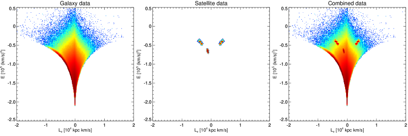
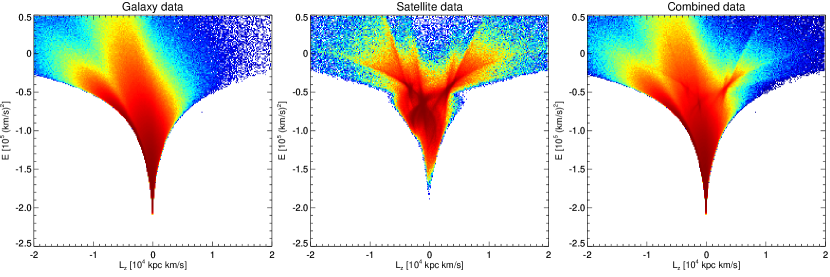
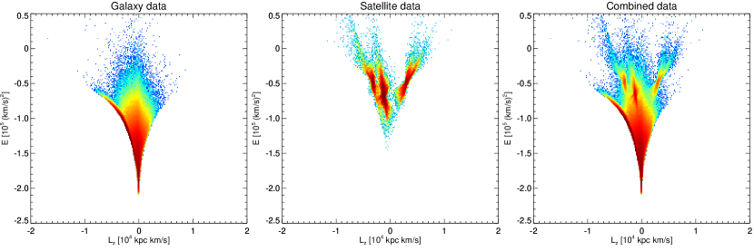
Figure 12: $E$–$L_{z}$ space for three of our disrupted $N$-body satellites and the synthetic Milky Way catalogue. The upper panels show the error free $E$–$L_{z}$ diagrams (from left to right: Galaxy stars only, satellite stars only, and Galaxy and satellite stars combined, respectively). The middle panels show $E$–$L_{z}$ space after the expected Gaia observational errors have been added. Only stars with radial velocities and positive measured parallaxes are plotted. Finally the lower panels show only the simulated stars from a high-quality sample for which $V<15$ and $\varpi/\sigma_{\varpi}>5$. These figures have been constructed as two-dimensional histograms by counting stars in 250$\times$250 cells that divide $E$–$L_{z}$ space. The white areas correspond to empty cells while the individual dots indicate cells with 1 or more stars. Areas where all contiguous cells are filled appear as a grey scale.

5.2 Searching for satellite remnants in $E$–$L_{z}$ space

We constructed $E$–$L_{z}$ diagrams for all of our satellite $N$-body simulations together with the synthetic catalogue of the background population associated with the Milky Way. For clarity in the following discussion we concentrate on just a few satellites. The diagrams are shown in Fig. 12. The upper panels refer to the $E$–$L_{z}$ diagrams without Gaia errors (from left to right: Galaxy only, satellites only and Galaxy and satellites combined). The middle panels show the effect of adding the expected Gaia observational errors. In this case the sample was restricted to stars with positive parallaxes and measured radial velocities in order to calculate $E$ and $L_{z}$. This selection criterion introduces an implicit limit on the apparent brightness of the stars of $V\la 17$–$18$. In the bottom panels the sample of stars selected from the catalogue is restricted to stars brighter than $V=15$ having a parallax signal-to-noise of $\varpi/\sigma_{\varpi}>5$ . In these diagrams, the entire Galaxy catalogue consists of $3.5\times 10^{8}$ stars and the satellite models correspond to runs 1 and 5 of Table 6 where a third satellite was generated by reversing the angular momentum of the satellite from run 1. All satellites have $M_{V,\mathrm{tracer}}\,=\,0.5$ (i.e. $M_{\mathrm{V,tot}}\approx-17$) and the stellar luminosities and colours were computed using a $10$ Gyr isochrone with metallicity $Z=0.004$ and a mass function $\xi(m)\propto m^{-1.5}$. Energies were computed employing the Galaxy model described in section 3.

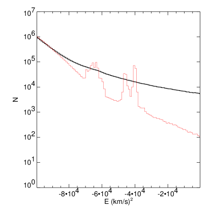
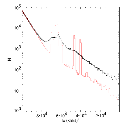
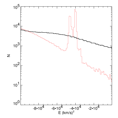
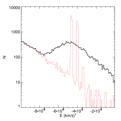
Figure 13: Energy histograms obtained from $E$–$L_{z}$ space for all satellite and Galaxy stars by taking slices in the integral of motion $L_{z}$. The leftmost two $E$-histograms correspond to all stars located in the interval $-7\times 10^{3}<L_{z}<0$ containing the prograde satellites (from left to right the entire and restricted Gaia samples, respectively). Similarly, the right two $E$-histograms were constructed by using the interval $10^{3}<L_{z}<7\times 10^{3}$ enclosing the retrograde satellite. In all cases, thin lines indicate error-free data while thick lines correspond to data after Gaia errors are added. Prograde satellites are centred at energies $E\approx-6.5\times 10^{4}$ (km s^-1)², $E\approx-4.2\times 10^{4}$ (km s^-1)²; the retrograde satellite is centred at energy $E\approx-4.2\times 10^{4}$ (km s^-1)².

In practice one will not know the actual potential of the Milky Way and thus an estimate of this quantity is required to calculate $E$. To simulate the effect of an erroneous estimate of the potential we also computed the energy using an alternative Galaxy potential model (see equations (8)–(10) of Helmi & de Zeeuw, 2000). This results in a larger spread of the Galaxy and satellite stars in energy and this spread can be used in combination with the angular momentum measurements and a detailed modelling of the identified debris streams in order to constrain the Galactic potential. However the $E$–$L_{z}$ diagrams with the observational errors included look largely the same as those in Fig. 12 so we will not consider this issue further in the discussion that follows.

It can be seen that satellite remnants are easy to identify if there are no observational errors, even in the presence of a stellar background (upper panels of Fig. 12). However, once the observational errors are introduced, the identification process becomes more difficult. Notice how the satellite and Galaxy stars are now smeared out in preferential directions in the $E$–$L_{z}$ diagram, which is caused by the dominance of the parallax errors as illustrated in Fig. 11. The middle panels of Fig. 12 demonstrate that if the entire Gaia Survey is taken into account it becomes very difficult to disentangle the different merger events. In particular, satellites on prograde orbits become buried in the very crowded region occupied by the Galactic disc. The identification process can be significantly improved when the search in $E$–$L_{z}$ is restricted to a ‘high quality’ sample as illustrated in the lower panels of Fig. 12. In this case, even a visual identification clearly shows all three satellites despite the presence of the Galactic stellar background. In this respect, the middle diagram of the lower panels in Fig. 12 is similar to Fig. 4 of Helmi & de Zeeuw (2000). However the clumping of the debris streams in $E$–$L_{z}$ is less clear and they are connected to each other by the background population of Milky Way stars. This makes the application of a ‘friends of friends’ algorithm to search for debris streams (as proposed by Helmi & de Zeeuw, 2000) less attractive.

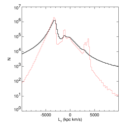
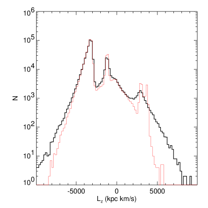
Figure 14: $L_{z}$ histograms obtained from $E$–$L_{z}$ space for all satellite and Galaxy stars by taking a slice in the integral of motion $E$. The left panel shows the $L_{z}$-histogram considering the whole survey in the energy interval $-10^{5}<E<0$ while the right panel shows the distribution of $L_{z}$ for our high quality sample in the same energy range. The lines have the same meaning as in Fig. 13.

Another very important feature of these $E$–$L_{z}$ diagrams is that the observational errors introduce a lot of false high density structures associated with the satellites (see middle column in Fig. 12). These structures look like singularities or caustics in phase-space and from a naive analysis could be mistaken for features in the topology of phase-space corresponding to physical entities or past merger events that in reality do not exist.

Taking slices in the integrals of motion by selecting certain ranges of $E$ or $L_{z}$ allows us to make a more quantitative assessment by focusing our attention on $E$ or $L_{z}$-histograms containing the relics of the disrupted satellites. A similar approach has been used by Meza et al. (2005) for the case of the debris of the $\omega$Cen dwarf, the galaxy that presumably contributed the $\omega$ Cen globular cluster to our galaxy. They were able to identify histogram peaks coinciding with the loss of satellite particles in the last three pericentric passages (see their fig. 4). However, our case proves to be more challenging, as can be appreciated in Figs. 13 and 14. Here the thin lines refer to error-free data and the thick lines to data after Gaia errors have been taken into account. $E$ histograms for error-free data show a double peak around each satellite. These peaks seems to be related to stars coming from the leading and trailing tails of the disrupted satellite. However, these peaks are smeared out over the entire energy space when Gaia errors are added, while only some bumps survive in our high quality sample (notice that even in this more favourable situation any trace of one of the prograde satellites has been completely erased). A similar behaviour is seen in the $L_{z}$ histograms, although in this case all three satellites are preserved after the errors are added in the high quality sample.

Finally, we note that dynamical friction has been ignored in our numerical simulations of satellite disruption. If dynamical friction is taken into account $L_{z}$ will not be conserved and its evolution will strongly depend on the initial satellite mass as well as on the orbital angular momentum with respect to the angular momentum of the main Galaxy. For example prograde orbits decay faster than retrograde ones (Huang & Carlberg, 1997; Velázquez & White, 1999). However, Helmi, White & Springel (2003) have pointed out that the conservation of phase-space density remains a promising technique for providing useful information about the Galaxy formation history even in a more realistic situation where an entire galaxy builds up from mergers in a $\Lambda$-CDM cosmology.

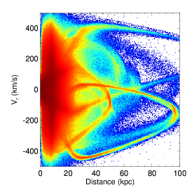
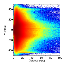
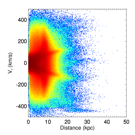
Figure 15: Radial velocity versus distance diagrams for our simulated Gaia catalogue. The same satellites as in Fig. 12 were used and superposed on the Galactic background. The left panels shows the data without observational errors. The middle panel shows the effect of adding the Gaia measurement errors, and the right panel shows the Gaia data for a high quality subsample restricted in magnitude, $V<15$, and parallax, signal-to-noise $\varpi/\sigma_{\varpi}>5$ as in Fig. 12. Note the change in the horizontal scale in this last panel. These figures were generated in the same way as Fig. 12.

5.3 Searching for satellite remnants in $r$–$v_{\mathrm{rad}}$ space

Johnston, Spergel & Hernquist (1995) suggested that diagrams of radial velocity versus distance would provide a powerful tool to look for fossil signatures in the halo of our Galaxy. These $r$–$v_{\mathrm{rad}}$ diagrams are related to the $E$–$L_{z}$ diagrams since, roughly speaking, the total energy of particles reflects the apocentre of the orbit while the pericentric radius is associated with the orbital angular momentum. This technique has not been applied in practice owing to a lack of data sets with enough radial velocities and reliable distances.

Figure 15 shows the $r$–$v_{\mathrm{rad}}$ diagrams for our simulated Gaia catalogue. The same satellites were used as for the $E$–$L_{z}$ diagrams. The data without the observational errors are shown in the left panel. The debris of the disrupted satellites can clearly be distinguished as narrow structures in this diagram but it is not possible to associate the latter with one or another of the satellites. When the observational errors are included most of these fossil signatures are washed out and a straightforward detection will be quite difficult as can be appreciated in the middle $r$–$v_{\mathrm{rad}}$ diagram. Restricting the data to the same high quality subsample as defined above, does not change the situation although it is possible to discern some structures related to the tidal debris left by the disrupted satellites.

5.4 The need for complementary search methods

These results show that a straightforward search for the debris of satellite galaxies in $E$–$L_{z}$ or $r$–$v_{\mathrm{rad}}$ space may not be very efficient in practice. A good start can be made by limiting the search to high quality samples, where the contrast between satellites and Galaxy can be further enhanced by concentrating on certain regions of the sky (away from the Galactic disc for example). However the effects of error propagation and selection biases (see Section 5.1) should be carefully accounted for. Once a first set of stars belonging to a particular remnant has been identified in $E$–$L_{z}$ one can in principle trace the rest of the stream by modelling the orbit of the satellite and by making use of the astrophysical properties of the stars (age, metallicity, alpha-element enhancements) which will be known from the photometric data provided by Gaia. Alternatively one can select samples of metal poor stars (thereby also lowering the Galaxy-satellite contrast) from the Gaia catalogue in order to study the very oldest remnants. Gaia will also provide extremely well calibrated photometric distances based on the parallaxes of the nearer and/or brighter stars. These calibrations can be used to obtain accurate distances for faint stars for which Gaia parallaxes are of poor quality. Better distances for the fainter stars will dramatically improve the quality of the $E$–$L_{z}$ and $r$–$v_{\mathrm{rad}}$ diagrams. These complementary procedures can be studied with our simulations by adding a more complete model of the Gaia photometric data.

6 Conclusions

Gaia will provide us with an unprecedented wealth of information on the structure and formation history of the Milky Way galaxy, for the first time providing full phase-space information across its entire volume. Exploiting this data set for studies of the assembly of the halo and other components of the Milky Way will be challenging owing to the enormous volume of data; astrometry and photometry for 1 billion stars and radial velocities for 100–150 million stars, over the entire sky. A good preparation will require familiarizing ourselves with the handling of such large datasets as well as exploring the best ways of disentangling remnants of past merger events from each other and from the Galactic background population.

We have started to address this problem by simulating the Gaia catalogue with a realistic number ($10^{8}$–$10^{9}$) of entries. This was done by combining a Monte Carlo model of the Milky Way with $N$-body simulations of satellites being disrupted as they orbit in the potential of our Galaxy. The Monte Carlo model of the Milky Way consists of $3.5\times 10^{8}$ stars and was generated by taking into account how the Gaia survey limit introduces magnitude limited spheres for each stellar type. The region on the sky limited by Galactic coordinates $-90^{\circ}\leq\ell\leq+90^{\circ}$ and $-5^{\circ}\leq b\leq+5^{\circ}$ was left out of the simulations for practical (computation time) reasons.

The models of the debris streams were generated by simulating the disruption of dwarf galaxies orbiting our galaxy. The Milky Way is represented by a rigid potential and a tree-code was used to carry out the $N$-body simulations of the orbiting satellites over a time period of about 10 Gyr. The simulations were carried out for satellites placed on five different orbits which vary in apocentre, pericentre and the initial inclination with respect to the Milky Way’s disc. Multiple debris streams can then be simulated by combining different $N$-body snapshots (different orbits and/or ages), and each snapshot can be rotated around the $Z$-axis, flipped with respect to the disc plane, or reversed in angular momentum.

We describe in detail how to correctly combine the Milky Way and satellite models such that the variation of the number of visible stars along the orbit of a satellite is taken into account. This is most easily achieved by assuming that the $N$-body particles represent a bright tracer population of a larger underlying dwarf galaxy.

After combining the models the synthetic Gaia catalogue was generated by adding the astrometric and radial velocity errors according to the prescriptions resulting from detailed preparatory studies of the Gaia mission. The observational errors were modelled taking into account the dependence on apparent magnitude, colour and sky position of the stars. To assign photometric properties to the particles we use a Hess diagram for the Solar neighbourhood for Galactic particles, while for the satellite particles we use isochrones from the Padova group. Our work thus introduces a thorough methodology to incorporate $N$-body simulations within a simulation of an actual observational survey in a manner that addresses questions of kinematics, metallicity and photometric properties of the simulated system, as well as errors in the observables.

The catalogue was used to study the appearance of the Galaxy and satellite data in $E$–$L_{z}$ space. The results show that it will be challenging to trace the debris streams throughout the entire volume of the Galaxy when Gaia errors are properly accounted for. However, limiting the sample to bright stars with good parallaxes allows a preliminary search to be done which should be followed up by complementing searches in $E$–$L_{z}$ by, for example, a further tracing of the debris streams based on the astrophysical properties of the stars which will be known from the photometry provided by Gaia. In addition, using photometric distances, which will be very well calibrated after the Gaia mission, will yield accurate distances for faint stars which can be used instead of the parallaxes, thus avoiding the problems associated with the propagation of parallax errors into the integrals of motion.

Ultimately our aim is to use these simulations to study much more thoroughly and realistically the possible search techniques one can use to recover the remnants of satellites in the stereoscopic and multi-colour data set that Gaia will provide. This includes a more complete study of the use of the integrals of motion method by also using the full angular momentum vector $L$ and a further exploration of the radial velocity versus distance diagrams. In addition we will explore how the astrophysical information from the Gaia photometry can be used in the search for debris streams. This requires a number of improvements to our simulations, which include:

• A proper model of the Gaia photometric system which is available using the tools developed by the Gaia Photometric Working Group (see Jordi & Høg, 2005; Carrasco et al., 2005).

• Updating the predicted Gaia observational errors to the latest available assessments. Specifically, the radial velocity errors we used are somewhat optimistic and a better assessment of them is now available (Katz et al., 2004).

• Using a clumped distribution of stars in the halo. The simulation of a clumpy halo will not be trivial and will probably require simulating multiple merger events which combine to form the halo. This may be obtained from the results of detailed cosmological simulations.

• Including an extinction model and possibly adding a thick disc to the Galaxy model. Within the Gaia project 3D extinction models have been developed which can be added to our simulations (see Drimmel, 2005).

• Using more sophisticated models for the dwarf galaxies. The $N$-body simulations should include dynamical friction and possibly more particles. The simulation of the stellar properties of the satellite particles should be updated with a more realistic mass function and possibly with the inclusion of more than one stellar population in the dwarf galaxy. The need for the latter is supported by the recent results concerning the stellar population of the Sculptor dwarf galaxy in which two distinct ancient stellar components were found (Tolstoy et al., 2004).

Appendix A Transforming Phase-Space Coordinates to Gaia Data

Here we describe in detail how the phase-space coordinates $(\mathbf{r},\mathbf{v})$ of our model Galaxy were converted to the data in the simulated Gaia catalogue; the five astrometric parameters $\ell$, $b$, $\varpi$, $\mu_{\ell*}$, and $\mu_{b}$ and the radial velocity $v_{\mathrm{rad}}$. The barycentric position $\mathbf{r}^{\mathrm{b}}=\mathbf{r}-\mathbf{r}_{\odot}$ and velocity $\mathbf{v}^{\mathrm{b}}=\mathbf{v}-\mathbf{v}_{\odot}$ are related to the astrometric and radial velocity data as follows (see e.g. ESA, 1997, Sections 1.2 and 1.5):

$$\mathbf{r}^{\mathrm{b}}=A_{p}\mathbf{\hat{r}}/\varpi$$ (12)

and:

$$\mathbf{v}^{\mathrm{b}}=\mathbf{\hat{p}}\mu_{\ell*}A_{v}/\varpi+\mathbf{\hat{q}}\mu_{b}A_{v}/\varpi+\mathbf{\hat{r}}v_{\mathrm{rad}}\,,$$ (13)

where $[\mathbf{\hat{p}}\ \mathbf{\hat{q}}\ \mathbf{\hat{r}}]$ is the normal triad defined below, and $A_{p}=1000$ mas pc and $A_{v}=4.74047...$ yr km s^-1 designate the astronomical unit in the appropriate form. Note that if the distances are in units of kpc, the units of parallax and proper motion are micro-arcsecond ($\mu$as) and micro-arcsecond per year ($\mu$as yr^-1).

In the galactic coordinate system the components of the normal triad $[\mathbf{\hat{p}}\ \mathbf{\hat{q}}\ \mathbf{\hat{r}}]$ are given by:

$$\mathsfbf{R} = \left(\begin{array}[]{ccc}p_{x}&q_{x}&r_{x}\\ p_{y}&q_{y}&r_{y}\\ p_{z}&q_{z}&r_{z}\end{array}\right)$$ (17)

$$= \left(\begin{array}[]{ccc}-\sin\ell&-\sin b\cos\ell&\cos b\cos\ell\\ \phantom{-}\cos\ell&-\sin b\sin\ell&\cos b\sin\ell\\ 0&\cos b&\sin b\end{array}\right)\,,$$ (21)

where $\mathbf{\hat{r}}$ is the unit vector that specifies the (instantaneous) barycentric coordinate direction $(\ell,b)$, and $\mathbf{\hat{p}}$ and $\mathbf{\hat{q}}$ are the unit vectors in the directions of increasing $\ell$ and $b$ at $\mathbf{\hat{r}}$. The galactic coordinate components of $\mathbf{r}^{\mathrm{b}}$ and $\mathbf{v}^{\mathrm{b}}$ may thus be written:

$$\left(\begin{array}[]{c}r^{\mathrm{b}}_{x}\\ r^{\mathrm{b}}_{y}\\ r^{\mathrm{b}}_{z}\end{array}\right)=\mathsfbf{R}\left(\begin{array}[]{c}0\\ 0\\ A_{p}/\varpi\end{array}\right)$$ (22)

and:

$$\left(\begin{array}[]{c}v^{\mathrm{b}}_{x}\\ v^{\mathrm{b}}_{y}\\ v^{\mathrm{b}}_{z}\end{array}\right)=\mathsfbf{R}\left(\begin{array}[]{c}\mu_{\ell*}A_{v}/\varpi\\ \mu_{b}A_{v}/\varpi\\ v_{\mathrm{rad}}\end{array}\right)$$ (23)

These equations can be inverted to calculate the astrometric and radial velocity data from the barycentric positions and velocities, yielding:

$$\varpi=A_{p}/|\mathbf{r}^{\mathrm{b}}|$$ (24)

and

$$\left(\begin{array}[]{l}v_{\ell*}\\ v_{b}\\ v_{\mathrm{rad}}\end{array}\right)=\mathsfbf{R}^{\prime}\left(\begin{array}[]{c}v^{\mathrm{b}}_{x}\\ v^{\mathrm{b}}_{y}\\ v^{\mathrm{b}}_{z}\end{array}\right)\,,$$ (25)

where $v_{\ell*}=\mu_{\ell*}A_{v}/\varpi$ and $v_{b}=\mu_{b}Av/\varpi$ are the velocity components perpendicular to the line of sight to the star, and $\mathsfbf{R}^{\prime}$ indicates the transpose of $\mathsfbf{R}$.

Table 7: Radial velocity precision (in km s^-1) as a function of stellar spectral type and magnitude $V$. These are the numbers used in our simulations, taken from Fig. 8.14 in ESA (2000).

OBA		FGKM
$V$	$\sigma_{v_{\mathrm{rad}}}$	$V$	$\sigma_{v_{\mathrm{rad}}}$
10	0.25	10	0.1
15	4	16	1
16	10	17	2
17	50	18	6

Once the astrometric data have been calculated from $\mathbf{r}$^b and $\mathbf{v}$^b they are transformed to the Ecliptic coordinate system before adding the astrometric errors. This is done to simulate the fact that the astrometric errors will vary over the sky as a function of the Ecliptic latitude $\beta$. As a consequence, upon rotation back to the Galactic reference frame, correlations are introduced between the errors in $\ell$ and $b$, and $\mu_{\ell*}$ and $\mu_{b}$. The transformation to the Ecliptic coordinate system is done through a rotation matrix as explained in Section 1.5.3 of the introductory volume to the Hipparcos and Tycho Catalogues (ESA, 1997).

The errors in the astrometry are then added as follows (see Perryman, 2002; ESA, 2000). The error on the parallax is given by:

$$\sigma_{\varpi}\simeq (7+105z+1.3z^{2}+6\times 10^{-10}z^{6})^{1/2}$$ (26)

$$\times[0.96+0.04(V-I)]\,,$$

where $z=10^{0.4(G-15)}$ and $G$ is the broad band Gaia magnitude (defined by the mirror reflectivity and CCD quantum efficiency curves) which can be calculated from the approximate transformation:

$$G= V+0.51-0.50\times\sqrt{0.6+(V-I-0.6)^{2}}$$ (27)

$$-0.065\times(V-I-0.6)^{2}\,.$$

For the mean position and proper motion errors $\sigma_{0}$ and $\sigma_{\mu}$ the following mean relations are used:

$$\sigma_{0}=0.87\sigma_{\varpi}\,,\quad\sigma_{\mu}=0.75\sigma_{\varpi}$$ (28)

Finally, the variations of the errors as a function of $\beta$ are taken from Table 8.3 in ESA (2000).

The errors on the radial velocity have been taken from fig. 8.14 in ESA (2000), which shows the radial velocity accuracy for a number of values of $V$ for both hot (OBA) and cool (FGKM) stars. The numbers are given in Table 7 and interpolation was used for intermediate values of $V$. For OBA stars fainter than $V=17$ and FGKM fainter than $V=18$ no radial velocities are generated.

Finally, the predicted observational errors for Gaia as quoted here reflect the estimates at the time the Gaia Concept and Technology Study Report was published (ESA, 2000). The values will evolve along with changes in the details of the mission design and implementation.

Appendix B Angular momentum from astrometric and radial velocity data

Because the Sun is not located at the centre of the Galaxy the relation between the angular momentum of a star and its measured position, parallax, proper motion and radial velocity is complicated by the necessity to transform from the barycentric to the Galactocentric frame. The angular momentum vector $\mathbf{L}$ is calculated as $\mathbf{r}\times\mathbf{v}=(\mathbf{r}^{\mathrm{b}}+\mathbf{r}_{\odot})\times(\mathbf{v}^{\mathrm{b}}+\mathbf{v}_{\odot})$, which when worked out using Eqs.(22) and (23) yields:

$$\mathbf{L}=\mathbf{L}^{\mathrm{g}}+\mathbf{L}^{\odot}\,,$$ (29)

where $\mathbf{L}^{\mathrm{g}}$ is given by:

$$\mathbf{L}^{\mathrm{g}}=\frac{A_{p}A_{v}}{\varpi^{2}}\begin{pmatrix}\phantom{-}\mu_{b}\sin\ell-\mu_{\ell*}\sin b\cos\ell\\[5.0pt] -\mu_{b}\cos\ell-\mu_{\ell*}\sin b\sin\ell\\[5.0pt] \mu_{\ell*}\cos b\end{pmatrix}\,,$$ (30)

and $\mathbf{L}^{\odot}$ is given by:

$$\mathbf{L}^{\odot}=\begin{pmatrix}-V_{\odot}\frac{A_{p}\sin b}{\varpi}\\[5.0pt] -R_{\odot}\left[\frac{A_{v}\mu_{b}\cos b}{\varpi}+v_{\mathrm{rad}}\sin b\right]\\[5.0pt] R_{\odot}\Lambda+\frac{A_{p}\cos b\cos\ell}{\varpi}V_{\odot}\end{pmatrix}\,,\\$$ (31)

where the term $\Lambda$ is given by:

$$\begin{split}\Lambda=&\frac{A_{v}\mu_{\ell*}\cos\ell}{\varpi}-\frac{A_{v}\mu_{b}\sin b\sin\ell}{\varpi}\\ &+v_{\mathrm{rad}}\cos b\sin\ell+V_{\odot}\,.\end{split}$$ (32)

$\mathbf{L}^{\mathrm{g}}$ is the ‘Galactocentric’ angular momentum which has no physical meaning but corresponds to the angular momentum calculated by an observer at the Galactic centre. The vector $\mathbf{L}^{\odot}$ indicates the components of the observed angular momentum that arise from the transformation from a barycentric to Galactocentric frame of reference. The norm of $\mathbf{L}^{\mathrm{g}}$ correctly evaluates to:

$$|\mathbf{L}^{\mathrm{g}}|=\frac{A_{p}A_{v}}{\varpi^{2}}\sqrt{\mu_{\ell*}^{2}+\mu_{b}^{2}}\,,$$ (33)

i.e., the distance to the Galactic centre multiplied by the total tangential velocity. The equation above shows how the radial velocity enters the angular momentum measurements and can be used to further study the way the astrometric errors propagate in the measured angular momentum.

The equations for the energy of a star can be worked out similarly but they depend on the model for the potential energy and hence we do not provide them here.

References

- Arnold & Gilmore (1992) Arnold R., Gilmore G., 1992, MNRAS, 257, 225
- Binney & Merrifield (1998) Binney J., Merrifield M., 1998, Galactic Astronomy, Princeton NJ, Princeton University Press
- Binney & Tremaine (1987) Binney J., Tremaine S., 1987, Galactic Dynamics, Princeton NJ, Princeton University Press
- Bond & Szalay (1983) Bond J. R., Szalay A. S., 1983, ApJ, 274, 443
- Brown et al. (1997) Brown A. G. A., Arenou F., van Leeuwen F., Lindegren L., Luri X., 1997, in Hipparcos Venice ’97, ESA SP-402, p. 681
- Bullock (2002) Bullock J. S., 2002, in Natarajan P., ed, The shapes of galaxies and their dark halos. Singapore, World Scientific, p. 109
- Carney et al. (1989) Carney B. W., Latham D., Laird J., 1989, AJ, 97, 423
- Carrasco et al. (2005) Carrasco J. M., Jordi C., Figueras F., Torra J., 2005, in Proceedings of the Symposium ‘The Three Dimensional Universe with Gaia’, ESA SP-576, p. 155
- Cole at al. (2000) Cole S., Lacey C. G., Baugh C. M., Frenk C. S., 2000, MNRAS, 319, 168
- Cox (2000) Cox A. N., ed, 2000, Allen’s Astrophysical Quantities, 4th ed., New York NY, AIP Press
- Cutri et al. (2003) Cutri R. M., et al. 2003, The 2MASS All-Sky Catalog of Point Sources, VizieR, II/246
- Dionidis & Beers (1989) Dionidis S. P., Beers T. C., 1989, ApJ, 340, L57
- Drimmel (2005) Drimmel R., 2005, in Proceedings of the Symposium ‘The Three Dimensional Universe with Gaia’, ESA SP-576, p. 167
- Dubinski (1994) Dubinski J., 1994, ApJ, 431, 617
- Dubinski (1996) Dubinski J., 1996, New Astronomy, vol. 1, 133
- Dubinski & Carlberg (1991) Dubinski J., Carlberg R. G., 1991, ApJ, 378, 496
- Eggen (1965) Eggen O. J., 1965, in Blaauw A., Schmidt M., eds, Galactic Structure, Stars and Stellar Systems, volume 5, University of Chicago Press, 111
- ESA (1997) ESA, 1997, The Hipparcos and Tycho Catalogues, ESA SP-1200
- ESA (2000) ESA, 2000, GAIA Concept and Technology Study Report, ESA-SCI(2000)4
- Feltzing, Gilmore & Wise (1999) Feltzing S., Gilmore G., Wyse R. F. G., 1999, ApJ, 516, L17
- Freeman & Bland-Hawthorn (2002) Freeman K., Bland-Hawthorn J., 2002, ARA&A, 40, 487
- Gilmore & Wyse (1985) Gilmore G., Wyse R. F. G., 1985, AJ, 90, 2015
- Girardi et al. (2000) Girardi L., Bressan A., Bertelli G., Chiosi C., 2000, A&AS 141, 371
- Girardi et al. (2002) Girardi L., Bertelli G., Bressan A., Chiosi C., Groenewegen M. A. T., Marigo P., Salasnich B., Weiss A., 2002, A&A, 391, 195
- Gorski et al. (1999) Gorski K. M., Hivon E., Wandelt B. D. 1999, in Banday A. J., Seth R. S., Da Costa L., eds, Proceedings of the MPA/ESO Cosmology Conference “Evolution of Large Scale Structure”, PrintPartners Ipskamp, The Netherlands, p. 37
- Helmi (2004) Helmi A., 2004, ApJ 610, L97
- Helmi & White (1999) Helmi A., White S. D. M., 1999, MNRAS, 307, 495
- Helmi & de Zeeuw (2000) Helmi A., de Zeeuw P. T., 2000, MNRAS 319, 657
- Helmi et al. (1999) Helmi A., White S. D. M., de Zeeuw P. T., Zhao H. S., 1999, Nat, 402, 53
- Helmi et al. (2002) Helmi A., White S. D. M., Springel V., 2002, Phys. Rev. D., vol. 66, Issue 6, id. 063502
- Helmi et al. (2003) Helmi A., White S. D. M., Springel V., 2003, MNRAS, 339, 834
- Huang & Carlberg (1997) Huang S., Carlberg R. G., 1997, ApJ, 480, 503
- Hernquist (1990) Hernquist L., 1990, ApJ, 356, 359
- Ibata, Gilmore & Irwin (1994) Ibata R., Gilmore G., Irwin M., 1994, Nature, 370, 194
- Ibata et al. (2001) Ibata R., Lewis G. F., Irwin M., Totten E., Quinn T.s, 2001, ApJ, 551, 294
- Irwin & Hatzidimitriou (1995) Irwin M., Hatzidimitriou D., 1995, MNRAS, 277, 1354
- Johnston et al. (1995) Johnston K. V., Spergel D. N., Hernquist L., 1995, ApJ, 451, 598
- Johnston et al. (1996) Johnston K. V., Hernquist L., Bolte M., 1996, ApJ, 465, 278
- Jordi & Høg (2005) Jordi C., Høg E., 2005, in Proceedings of the Symposium ‘The Three Dimensional Universe with Gaia’, ESA SP-576, p. 43
- Katz et al. (2004) Katz D., Munari U., Cropper M., Zwitter T., Thévenin F., David M., Viala Y., Crifo F., Gomboc A., Royer F., 2004, MNRAS, 354, 1223
- Kauffmann & White (1993) Kauffmann G., White S. D. M., 1993, MNRAS, 261, 921
- Kauffmann, White & Guiderdoni (1993) Kauffmann G., White S. D. M., Guiderdoni B., 1993, MNRAS, 264, 201
- King (1966) King I., 1966, AJ, 71, 64
- Klypin et al. (1999) Klypin A., Kravstov A. V., Valenzuela O., Prada F., 1999, ApJ, 522, 82
- Lynden-Bell (1976) Lynden-Bell D., 1976, MNRAS, 174, 695.
- Majewski, Munn & Hawley (1996) Majewski S. R., Munn J. A., Hawley S. L., 1996, ApJ, 459, L73
- Majewski et al. (2000) Majewski S. R., Ostheimer J. C., Kunkel W. E., Patterson R. J., 2000, AJ, 120, 2550
- Majewski et al. (2003) Majewski S. R., Skrutskie M. F., Weinberg M. D., Ostheimer J. C., 2003, ApJ, 599, 1028
- Martin et al. (2004) Martin N. F., Ibata R. A., Bellazinni M., Irwin M. J., Lewis G. F., Dehnen W., 2004, MNRAS, 348, 12
- Martínez-Delgado et al. (2004) Martínez-Delgado D., Gómez-Flechoso M. A., Aparicio A., Carrera R., 2004, ApJ, 601, 242
- Mateo (1998) Mateo M., 1998, ARA&A, 36, 435
- Meza et al. (2005) Meza A., Navarro J. F., Abadi M. G., Steinmetz M., 2005, MNRAS, in press (astro-ph/0408567)
- Mihalas & Binney (1981) Mihalas D., Binney J., 1981, Galactic Astronomy: Structure and Kinematics, 2nd ed., New York NY, W.H. Freeman and Company
- Monkiewicz et al. (1999) Monkiewicz J., et al., 1999, PASP, 111, 1392
- Moore et al. (1999) Moore, B., Ghigna, S., Governato, F., Lake, G., Quinn, T., Stadel, J., Tozzi, P., 1999, ApJL, 524, L19
- Morrison et al. (2000) Morrison H. L., Mateo M., Olszewski E. W., Harding P., Dohm-Palmer R. C., Freeman K. C., Norris J. E., Morita M., 2000, AJ, 119, 2254
- Navarro, Frenk & White (1997) Navarro J. F., Frenk C. S., White S. D. M., 1997, ApJ, 490, 493
- Newberg et al. (2002) Newberg H. J., et al., 2002, ApJ, 569, 245
- Oh et al. (1995) Oh K. S., Lin D. N. C., Aarseth S. J., 1995, ApJ, 442, 142
- Palma et al. (2003) Palma C., Majewski S. R., Siegel M. H., Patterson R. J., Ostheimer J. C., Link R., 2003, AJ, 125, 1352
- Paresce & De Marchi (2000) Paresce F., De Marchi G., 2000, ApJ, 534, 870
- Perryman (2002) Perryman M. A. C., 2002, in Bienaymé O., Turon. C., eds, GAIA: a European Space Project, EAS Pub. Ser. Vol. 2, EDP Sciences, Les Ulis, p. 3
- Perryman et al. (2001) Perryman M. A. C., de Boer K. S., Gilmore G., Høg E., Lattanzi M. G., Lindegren L., Luri X., Mignard F., Pace O., de Zeeuw P. T., 2001, A&A, 369, 339
- Press et al. (1992) Press W. H., Teukolsky S. A., Vetterling W. T., Flannery B. P., 1992, Numerical Recipes in Fortran: The Art of Scientific Computing, Second Edition, Cambridge University Press
- Quinn & Goodman (1986) Quinn P. J., Goodman J., 1986, ApJ, 309, 472
- Ratnatunga & Freeman (1985) Ratnatunga K., Freeman K. C., 1985, ApJ, 291, 260
- Rocha-Pinto et al. (2004) Rocha-Pinto H. J., Majewski S. R., Skrutskie M. F., Crane J. D., Patterson R. J., 2004, ApJ, 615, 732
- Rodgers & Paltoglou (1984) Rodgers A. W., Paltoglou G., 1984, ApJ, 283, L5
- Schröder et al. (2004) Schröder S. E., Kaper L., Lamers H. J. G. L. M., Brown A. G. A., 2004, A&A, 428, 149
- Somerville & Primack (1999) Somerville R. S., Primack J. R., 1999, MNRAS, 310, 1087
- Stockton et al. (2004) Stockton A., Canalizo G., Maihara T., 2004, ApJ, 605, 37
- Tecza et al. (2004) Tecza M., Baker A. J., Davies R. I., Genzel R., Lehnert M. D., Eisenhauer F., Lutz D., Nesvadba N., Seitz S., Tacconi L. J., Thatte N. A., Abuter R., Bender R., 2004, ApJ, 605, L109
- Tolstoy et al. (2004) Tolstoy E., et al., 2004, ApJ, 617, L119
- Vader & Chaboyer (1994) Vader J. P., Chaboyer B., 1994, AJ, 108, 1209
- Velázquez & White (1999) Velázquez H., White S. D. M., 1999, MNRAS, 304, 254
- Velázquez & Aguilar (2003) Velázquez H., Aguilar L. A., 2003, Rev. Mex. Astron. Astrof., 39, 197
- Wilkinson et al. (2002) Wilkinson M. I., Kleyna J., Evans N. W., Gilmore G., 2002, MNRAS 330, 778
- Wyse (1999) Wyse R. F. G., 1999, in Gibson B. K., Axelrod T. S., Putman M. E., eds, ‘Third Stromlo Symposium: The Galactic Halo’, ASP Conf. Series, Vol. 165, p. 1
- York et al. (2000) York D. G., et al., 2000, AJ, 120, 1579