Estimating Dark Matter Distributions

Abstract

Thanks to instrumental advances, new, very large kinematic datasets for nearby dwarf spheroidal (dSph) galaxies are on the horizon. A key aim of these datasets is to help determine the distribution of dark matter in these galaxies. Past analyses have generally relied on specific dynamical models or highly restrictive dynamical assumptions. We describe a new, non-parametric analysis of the kinematics of nearby dSph galaxies designed to take full advantage of the future large datasets. The method takes as input the projected positions and radial velocities of stars known to be members of the galaxies, but does not use any parametric dynamical model, nor the assumption that the mass distribution follows that of the visible matter. The problem of estimating the radial mass distribution, $M(r)$ (the mass interior to true radius $r$), is converted into a problem of estimating a regression function non-parametrically. From the Jeans Equation we show that the unknown regression function is subject to fundamental shape restrictions which we exploit in our analysis using statistical techniques borrowed from isotonic estimation and spline smoothing. Simulations indicate that $M(r)$ can be estimated to within a factor of two or better with samples as small as 1000 stars over almost the entire radial range sampled by the kinematic data. The technique is applied to a sample of 181 stars in the Fornax dSph galaxy. We show that the galaxy contains a significant, extended dark halo some ten times more massive than its baryonic component. Though applied here to dSph kinematics, this approach can be used in the analysis of any kinematically hot stellar system in which the radial velocity field is discretely sampled.

1 Introduction

Despite their humble appearances, the dwarf spheroidal (dSph) satellites of the Milky Way provide a source of persistent intrigue. Mysteries concerning their origin, evolution, mass density, and dynamical state make it difficult to know where to place these common galaxies in the context of standard (e.g. Cold Dark Matter) models of structure formation. Are they primordial building blocks of bigger galaxies, or debris from galaxy interactions?

While dSph galaxies have stellar populations similar in number to those of globular clusters ($M_{Lum}\sim 10^{6-7}M_{\odot}$), their stars are spread over a much larger volume ($R\sim 2$-$6$ kpc compared to $10$-$50$ pc in globular clusters) resulting in the lowest luminosity (i.e., baryonic) densities known in any type of galaxy. In many cases it is unclear how these galaxies could have avoided tidal disruption by the Milky Way over their lifetimes without the addition of considerable unseen mass. This characteristic of dSph galaxies suggests that the dynamics of these systems are dominated either by significant amounts of unseen matter, or that these galaxies are all far from dynamical equilibrium.

In general, the Jeans Equations (Equations (4-21), (4-24), and (4-27) of Binney & Tremaine 1987 BT87 , hereafter, BT87) provide a robust description of the mass distribution, $M(r)$, of a collisionless gravitational system – such as a dSph galaxy – in viral equilibrium, Equation (5) below. Their general form permits any number of mass components (stellar, gas, dark), as well as anisotropy in the velocity dispersion tensor and a non-spherical gravitational potential. When applied to spherical stellar systems and assuming at most only radial or tangential velocity anisotropy, these equations can be simplified to estimate the radial mass distribution (Equation 4-55 of BT87):

$$M(r)=-\frac{r\overline{{v_{r}}^{2}}}{G}\biggl{(}\frac{\operatorname{d}\operatorname{ln}\nu}{\operatorname{d}\operatorname{ln}r}+\frac{\operatorname{d}\operatorname{ln}\overline{{v_{r}}^{2}}}{\operatorname{d}\operatorname{ln}r}+2\beta\biggr{)},$$ (1)

where $\nu$ is the spatial density distribution of stars, $\overline{{v_{r}}^{2}}$ is the mean squared stellar radial velocity at radius $r$. The dimensionless isotropy parameter, $\beta(r)$, compares the system’s radial and tangential velocity components:

$$\beta\equiv 1-\frac{\overline{{v_{\theta}}^{2}}}{\overline{{v_{r}}^{2}}}.$$ (2)

Apart from the constraints on the geometry and the functional form of the anisotropy, Equation (1) is model-independent, making it an appealing tool. It is relevant that Equation (1) and (6) below are applicable to any tracer population that in equilibrium and satisfies the collisionless Boltzman Equation.

Kinematic datasets for individual dSph galaxies have historically been far too small (typically containing radial velocities for $\sim$ 30 stars; see Mateo 1998) to allow for a precise determination of $M(r)$ using relations similar to Equation (1). Instead, authors have been forced to adopt additional strong assumptions that reduce the Jeans Equation to even simpler forms and where the relevant distributions ($\nu(r)$ and $\overline{v_{r}^{2}}(r)$ in Equation 1) are represented by parametric models. Specifically, if one assumes isotropy of the velocity dispersion tensor (i.e., $\beta=0$), spherical symmetry, and that the starlight traces the mass distribution (effectively a single-component King model (Irwin and Hatzidimitriou 1995)), then one obtains for the M/L ratio (Richstone and Tremaine 1986):

$${{M}\over{L}}=\eta{{9\sigma^{2}_{0}}\over{2\pi GI_{0}R_{h}}},$$ (3)

where $\sigma_{0}$ is the one-dimensional central velocity dispersion, $I_{0}$ is the central surface brightness, and $R_{h}$ is the half-light radius. The parameter $\eta$ is nearly equal to unity for a wide range of realistic spherical dynamical models so long as the mass distribution is assumed to match that of the visible matter. With this approach – the modern variant of the classical ‘King fitting’ procedure (King 1966) – the measured central radial velocity dispersion and surface brightness yield estimates of such quantities as the global and central M/L ratios. In all eight of the MW’s measured dSphs, large central velocity dispersions have conspired with their low surface brightnesses to produce large inferred M/L values. This line of reasoning has led to a general belief that dSph galaxies are almost completely dark-matter dominated, and their halos have assumed the role of the smallest non-baryonic mass concentrations identified so far in the present-day Universe.

This analysis fails for galaxies that are far from dynamical equilibrium, for example due to the effects of external tidal forces from the Milky Way (Fleck and Kuhn 2003; Klessen and Kroupa, 1998). Numerical models aimed to investigate this (Oh et al. 1995; Piatek and Pryor 1995) generally found that tides have negligible effects on the central dynamics of dSph galaxies until the survival time of the galaxy as a bound system becomes comparable to the orbital time (about 1 Gyr for the closer dSph satellites of the Milky Way). Observations agree with this broad conclusion by finding that remote dSph galaxies are no less likely to contain significant dark matter halos than systems located closer to their parent galaxy (Mateo et al. 1998; Vogt et al. 1995). However, so-called resonance models (Fleck and Kuhn 2003; Kuhn 1993; Kuhn et al. 1996) have been proposed that imply the central velocity dispersions can be significantly altered due to the inclusion of stars streaming outward from the barycenter of a galaxy and projected near the galaxy core. Recent versions of these models invariably imply a significant extension of the affected galaxies along the line-of-sight (more precisely, along the line between the center of the dwarf and the Milky Way; Kroupa 1997; Klessen and Kroupa 1998) and a massive tidal stream along the satellite’s orbit. Observations do not reveal strong evidence of significant line-of-sight distortions in dSph galaxies (Hurley-Keller et al 1999; Klessen et al. 2003), other than Sagittarius (e.g. Ibata et al. 1995); thus, for the purposes of this paper, we will assume that dSph galaxies are generally close to a state of dynamical equilibrium.

Even with this enabling assumption, the classical analysis of dSph masses as we describe it above is far from ideal for a number of reasons. First, though recent work (e.g. Irwin and Hatzidimitriou 1995) has helped to greatly improve estimates of dSph structural parameters ($I_{0}$ and $R_{h}$ in Equation 3), the errors in the velocity dispersions – often dominated by Poisson uncertainties due to the small number of kinematic tracers – contribute the principle source of uncertainty in M/L estimates. Second, there is little reason to suppose the assumption that mass follows light in dSphs is valid. In all other galaxies the bulk of the matter resides in a dark halo extending far beyond the luminous matter, a trend that becomes more exaggerated toward smaller scales (Kormendy and Freeman 2004). Finally, velocity anisotropies, if they exist, may mimic the presence of dark matter, and so represent a tricky degeneracy in the model even if the assumption of isotropy is dropped.

Modern instrumentation is poised to deliver dramatically larger kinematic datasets to help minimize the first problem. For example, the Michigan/Magellan Fiber System, now operational at the Magellan 6.5-m telescopes, obtains spectra from which high-precision radial velocities can be measured of up to 256 objects simultaneously. As a result, it is now feasible to obtain thousands of individual stellar spectra in many dSph systems, enlarging sample sizes by more than an order of magnitude. This not only reduces the statistical uncertainty of the dispersion estimation, but can also provide information on the spatial variation of the dispersion across the face of a galaxy. These rich datasets therefore allow for fundamentally improved results even using fairly conventional analysis techniques. For example, by parameterizing the velocity anisotropy, Wilkinson et al. (2002) and Kleyna et al. (2002) show that samples of $\sim 200$ stars can begin to break the degeneracy between anisotropy and mass in spherical systems.

But these large datasets also allow us to aim higher. In this paper, we introduce and develop the formalism for a qualitatively different sort of analysis designed to make the most efficient use of large kinematic datasets. Rather than adopting a model that parameterizes the various distributions used in the Jeans equation (e.g., $M(r)$, $\nu(r)$, $\overline{v_{r}^{2}}$, or $\beta(r)$), we operate on the star count and radial velocity data directly to estimate the mass distribution non-parametrically. We estimate the true three-dimensional mass distribution from the projected stellar distribution and the line-of-sight velocity distribution. In this first application of our technique, we still require the assumptions of viral equilibrium, spherical symmetry, and velocity isotropy ($\beta=0$). In Section 2, we introduce notation and definitions of the three-dimensional as well as projected stellar and phase-space densities and review the Jeans Equation. In Sections 3 and 4, we show how to use very general shape constraints on the mass distribution to estimate the detailed form of the velocity dispersion profile and the radial mass distribution. We illustrate the process on simulated data, demonstrating that, when furnished with large datasets, nonparametric analysis is a powerful and robust tool for estimating mass distributions in spherical or near-spherical systems (Section 5). We illustrate the application of our approach to an existing – but relatively small – kinematic dataset for the Fornax dSph galaxy at the end of Section 5.

Our emphasis in this paper is the application of our technique to dSph kinematics, but the method described in this paper is applicable to any dynamically hot system in which the radial velocity field is sampled discretely at the positions of a tracer population. Thus, our methodology would work for, say, samples of globular clusters or planetary nebulae surrounding large elliptical galaxies, or for individual stars within a globular cluster. Our approach follows earlier non-parametric analysis of globular cluster kinematics by Gebhardt and Fischer (1995) and Merritt et al. (1997), though the details of our method differ significantly.

2 Jeans’ Equation

Let $\mbox{\boldmath$X$}=(X_{1},X_{2},X_{3})$ and $\mbox{\boldmath$V$}=(V_{1},V_{2},V_{3})$ denote the 3-dimensional position and velocity of a star within a galaxy. We will regard these as jointly distributed random vectors, as in BT87, p. 194. Suppose that $X$ and $V$ have a joint density that is spherically symmetric and isotropic, so that

$$P[{\mbox{\boldmath$x$}}\leq{\mbox{\boldmath$X$}}\leq{\mbox{\boldmath$x$}}+d{\mbox{\boldmath$x$}}\ \&\ {\mbox{\boldmath$v$}}\leq{\mbox{\boldmath$V$}}\leq{\mbox{\boldmath$v$}}+d{\mbox{\boldmath$v$}}]=f_{0}(r,v)d{\mbox{\boldmath$x$}}d{\mbox{\boldmath$v$}},$$ (4)

where $r^{2}=x_{1}^{2}+x_{2}^{2}+x_{3}^{2}$ and $v^{2}=v_{1}^{2}+v_{2}^{2}+v_{3}^{2}$. We also suppose that $V$ has been centered to have a mean of zero so that $\int{\mbox{\boldmath$v$}}f_{0}(r,v)d{\mbox{\boldmath$x$}}d{\mbox{\boldmath$v$}}=0.$ Suppose finally that the mass density $\rho(r)$ is spherically symmetric and let

$$M(r)=4\pi\int_{0}^{r}t^{2}\rho(t)dt,$$ (5)

the total mass within $r$ of the center. The goal of this paper is to come up with a means of estimating $M(r)$ non-parametrically, specifically without assuming any special functional form for $f_{0}(r,v)$ or $\rho(r)$. In the presence of spherical symmetry, the relevant form of the Jeans Equation is

$$M(r)=-{r^{2}\mu(r)\over G}{d\over dr}\log\big{[}f(r)\mu(r)\big{]},$$ (6)

where

$$\mu(r)={1\over 3f(r)}\int v^{2}f_{0}(r,v)d\mbox{\boldmath$v$}$$ (7)

and

$$f(r)=\int f_{0}(r,v)d\mbox{\boldmath$v$}.$$

In statistical terminology, $\mu(r)$ is the conditional expectation of $V^{2}=(V_{1}^{2}+V_{2}^{2}+V_{3}^{2})/3$ given $x$ (this is the same as the conditional expectation on $V_{3}^{2}$, hence the factor of 3), and the marginal density of $X$ is $f(r)$. In astronomical terms, $\mu(r)$ is the one-dimensional radial-velocity dispersion profile squared, and $f(r)$ is the true, three-dimensional density profile of the tracer population. Using the notation of BT87, these correspond to $\overline{v_{r}^{2}}$ and $\nu(r)$, respectively.

To estimate $M(r)$ from equation (6) clearly requires estimates of the functions $f$ and $\mu$. For dSph galaxies, the data available for this consist of a large sample of positions and photometry of stars in individual systems (Irwin and Hatzidimitriou 1995; hereafter IH95), and much smaller samples of stars with positions and velocities (e.g. Walker et al. 2004). Of course, it is not possible yet to determine complete three-dimensional positional or velocity information for any of these stars, but only the velocity in the line of sight and the projection of position on the plane orthogonal to the line of sight. With a proper choice of coordinates, these observables become $X_{1},X_{2}$, and $V_{3}$. These can be made equivalent to, say, right ascension and declination, and radial velocity, respectively. The incomplete observation of $V$ does not cause a problem here, given the assumed isotropy, since $v^{2}$ can be replaced by $3v_{3}^{2}$ in Equation (7) without changing the value of $\mu(r)$. The incomplete observation of position poses a more serious problem that is known as Wicksell’s (1925) Problem in the statistical literature. The procedures for estimating $f$ and $\mu$ are consequently different; they will be considered separately in Sections 3 and 4.

3 The Spatial Distribution of Stars: Estimating $f$

Let $R=\sqrt{X_{1}^{2}+X_{2}^{2}+X_{3}^{2}}$ and $S=\sqrt{X_{1}^{2}+X_{2}^{2}}$ denote the true three-dimensional distance of a star and its two-dimensional projected distance from the origin, respectively. We denote the corresponding densities as $f_{\bf R}$ and $g_{\bf S}$. Then $f_{\bf R}(r)=4\pi r^{2}f(r)$, and

$$g_{\bf S}(s)=4\pi s\int_{s}^{\infty}{f(r)rdr\over\sqrt{(r^{2}-s^{2})}}.$$ (8)

For an example, consider Plummer’s distribution,

$$f_{0}(r,v)={c_{0}\over b^{5}}\left[{b\over\sqrt{1+{1\over 3}r^{2}}}-{1\over 2}v^{2}\right]_{+}^{7\over 2},$$ (9)

where $c_{0}$ is a constant,and $b$ is a parameter that is related to the velocity dispersion through $E(V^{2}|R=r)={b/[2\sqrt{1+r^{2}/3}]}$. Here $r$ is measured in units of 100 pc and $v$ in km/s. We also employ here the notation $[x]_{+}$ to denote taking the larger of $x$ and $0$. With this definition, we take $[x]_{+}^{\alpha}$ to be shorthand for $([x]_{+})^{\alpha}$; that is, the value of $x$ is either positive or zero before raising to the power $\alpha$. For this case, $f_{\bf R}(r)=r^{2}/[\sqrt{3}\sqrt{(1+r^{2}/3)^{5}}]$ and $g_{\bf S}(s)=2s/[3(1+s^{2}/3)^{2}]$. We use the Plummer distribution in our simulations below.

IH95 provide data from which $f$ can be estimated. These data consist of a sample of stars with projected radii $S_{1},\cdots,S_{N}$ and counts $N_{k}$ of the number of stars for which $r_{k-1}<S\leq r_{k}$ where $0=r_{0}<r_{1}<\cdots<r_{m}$ divide the stars into bins. Let $G_{\bf S}$ denote the distribution function of $S$, so that $G_{\bf S}(s)=P[S\leq s]=\int_{0}^{s}g_{\bf S}(t)dt$. Then $G_{\bf S}(r_{k})$ may be estimated from its empirical version

$$G_{\bf S}^{\#}(r_{k})={N_{1}+\cdots,+N_{k}\over N}.$$ (10)

In this context and throughout this paper, the $\#$ symbol denotes functions estimated directly from empirical data. Since the samples of stars used by IH95 to determine the surface density of most of the Milky Way dSph galaxies are quite large, there is generally very little statistical uncertainty in our estimate of $G^{\#}_{\bf S}$ from Equation (10). If we now model $f$ by a step function, say $f(r)=f_{k}$ for $r_{k-1}<r\leq r_{k}$ and $k=1,\cdots,m$, then $f_{1},\cdots,f_{m}$ may be recovered directly. In this case, the integral in Equation (8) is easily computed leading to

$$1-G_{\bf S}(r_{j-1})=\sum_{k=j}^{m}a_{jk}f_{k},$$

where

$$a_{jk}={4\pi\over 3}\big{[}\sqrt{(r_{k}^{2}-r_{j-1}^{2})^{3}}-\sqrt{(r_{k-1}^{2}-r_{j-1}^{2})^{3}}\big{]}.$$

Then $f_{1},\cdots,f_{m}$ may be recovered from

$$f_{j}={1\over a_{jj}}\big{[}1-G_{\bf S}(r_{j-1})-\sum_{k=j+1}^{m}a_{jk}f_{k}\big{]}.$$ (11)

The summation is to be interpreted to be zero when $j=m$, and the right side of equation (11) can in practice be estimated by replacing $G_{\bf S}$ with its empirical version $G_{\bf S}^{\#}$.

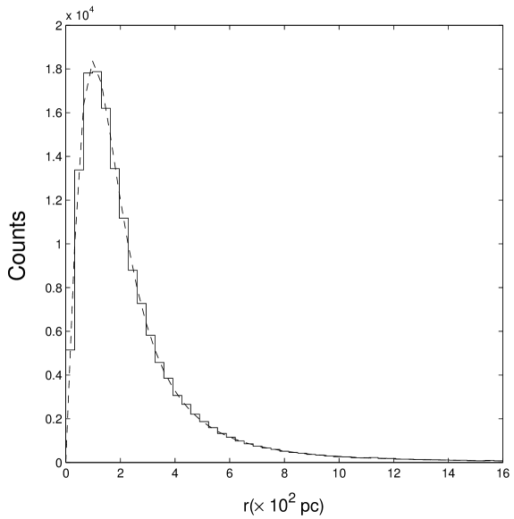
Figure 1: Simulated projected counts for 150,000 stars drawn from a Plummer model. The histogram shows the distribution of selected stars from this model; the dotted line shows the actual distribution defined by the model.

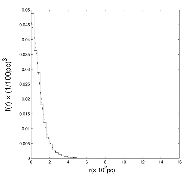
Figure 2: The function $f$ derived from the counts shown in Figure 1 derived using Equation (11) and for a sample size of 150,000 positions derived from a Plummer model. The true distribution is shown as a dashed line.

The results of applying this method to a sample of 150,000 positions drawn from a Plummer model with $b=200\times 3.1\times 10^{15}km^{3}/sec^{2}$ are shown in Figures 1 and 2. Figure 1 shows simulated counts of the number of stars in equally-spaced bins ranging from $0=r_{0}\leq r_{1}\leq\cdots\leq r_{50}=16\times 100pc$ . The estimate of $f$ from these simulated data is shown in Figure 2. In both figures the dotted line denotes the true function.

The estimation of $f$ follows Wicksell’s (1925) original analysis and can almost certainly be improved. We have not done that here, because the sample sizes are so large, but related questions are currently under investigation by Pal (2004).

4 Velocity Dispersion Profile: Estimating $\mu$ and $M$

For estimating $\mu$ and $M$ it is convenient to work with squared radius $Y=S^{2}=X_{1}^{2}+X_{2}^{2}$, as in Groeneboon and Jongbloed (1995) and Hall and Smith (1992). The joint density of $(Y,\mbox{\boldmath$V$})$ is then

$$g_{Y,\bf V}(y,{\mbox{\boldmath$v$}})=\pi\int_{y}^{\infty}{f_{0}(\sqrt{z},v)\over\sqrt{z-y}}dz.$$ (12)

Relation (7) represents a special case on integrating over all three velocity components and using $g_{\bf{S}}(s)=2sg_{\bf{Y}}(s^{2})$. Now let

$$\phi(z)=\int v_{3}^{2}f_{0}(\sqrt{z},v)\bf{dv},$$

and

$$\psi(y)=\int v_{3}^{2}g_{Y,\bf{V}}(y,\bf{v})d\mbox{\boldmath$v$},$$

so that $\psi(y)/g_{Y}(y)$ is the conditional expectation of $V_{3}^{2}$ given $Y=y$, and similarly for $\phi$. We also define the important function

$$\Psi(y)=\int_{y}^{\infty}{\psi(t)dt\over\sqrt{t-y}}.$$

Then, reversing the orders of integration and recognizing a beta integral (see BT87, p. 205), we can write

$$\Psi(y)=\pi^{2}\int_{y}^{\infty}\phi(z)dz$$ (13)

and

$$\phi(z)=-{1\over\pi^{2}}\Psi^{\prime}(z),$$ (14)

where the prime notation (^′) denotes the derivative. Clearly, $f(r)\mu(r)=\phi(r^{2})$ in Equation (7). Thus, the expression for $M(r)$ from the Jeans equation (Equation (6)) can be rewritten as

$$M(r)={2r^{3}\over G\pi^{2}}{\Psi^{\prime\prime}(r^{2})\over f(r)}.$$ (15)

Our estimator for $f$ was obtained in Section 3, so we focus here on determining $\Psi^{\prime\prime}$. For our problem, we benefit from noting that the function $\Psi$ is subject to certain shape restrictions which are useful in the estimation process. From Equation (13) we can see that $\Psi$ is a non-negative decreasing function, while from Equation (15) it is evident that $\Psi$ has a non-negative second derivative (that is, it is upward convex). In fact, $r^{3}\Psi^{\prime\prime}(r^{2})/f(r)$ must be an increasing function that vanishes when $r=0$, physically consistent with its direct proportionality to $M(r)$ in Equation (15).

The next step in the estimation of $M(r)$ is to estimate $\Psi$. Suppose that there is a sample $(X_{i,1},X_{i,2},U_{i}),\ i=1,\cdots,n$ of projected positions $(X_{i,1},X_{i,2})$ and radial velocities $U_{i}$ measured with known error, $\epsilon_{i}$. Thus, $U_{i}=V_{i,3}+\epsilon_{i}$, where where $\epsilon_{1},\cdots,\epsilon_{n}$ are independent of $(X_{i,1},X_{i,2},V_{i,3}),\ i=1,\cdots,n$ with zero mean values and known variances, $\sigma_{1}^{2},\cdots,\sigma_{n}^{2}$. In practice, there may be selection effects: An astronomer may choose to sample some regions of a galaxy more intensely than others, or external factors (weather, moonlight, telescope/instrument problems) may cause undersampling of some regions. To address this, we must include a selection function, $w_{0}(x_{1},x_{2})$, into the model. Here, $w_{0}(x_{1},x_{2})$ is the probability that a star in a galaxy is included in the kinematic sample, given that it is there. Thus the selection probability is assumed to depend on projected position, $(x_{1},x_{2})$, only. As before, let $Y_{i}=X_{i,1}^{2}+X_{i,2}^{2}$; then the joint density of $Y_{i}$ and ${\mbox{\boldmath$V$}}_{i}$ in the sample is

$$g_{{\bf Y,V}}^{*}(y,{\mbox{\boldmath$v$}})=w(y)g_{{\bf Y,V}}(y,{\mbox{\boldmath$v$}}),$$ (16)

where

$$w(y)={1\over c}\int_{-\pi}^{\pi}w_{0}[\sqrt{y}\cos(\theta),\sqrt{y}\sin(\theta)]d\theta,$$

$g_{{\bf Y,V}}$ is as in Equation (12 ), and $c$ is a normalizing constant, determined by the condition that the integral of $g_{{\bf Y,V}}^{*}(y,{\mbox{\boldmath$v$}})$ be one. Integrating over $v$ in (16), the actual density of $Y$ is

$$g_{{\bf Y}}^{*}(y)=w(y)g_{{\bf Y}}(y),$$ (17)

and $c$ is determined by the condition that $\int g_{\bf Y}^{*}(y)dy=1$. Here $g_{\bf Y}$ may be determined from the complete photometric data for a given galaxy to give the projected stellar distribution as a function of $Y$. If $f$ is a step function, then combining equations (8) and (11) with the relation $g_{\bf S}(s)=2sg_{\bf Y}(s^{2})$ leads to

$$g_{\bf Y}(y)=2\pi\left[f_{j}\sqrt{r_{j}^{2}-y}+\sum_{k=j+1}^{m}f_{k}\left(\sqrt{r_{k}^{2}-y}-\sqrt{r_{k-1}^{2}-y}\right)\right]$$

in the interval $r_{j-1}^{2}\leq y\leq r_{j}^{2}$ for $j=1,\cdots,m$. If an astronomer can specify $w_{0}(x_{1},x_{2})$, then $c$ and $w(y)$ can be computed directly using Equation (15). Then

$$\Psi^{\#}(z)={1\over n}\sum_{i:Y_{i}>z}{U_{i}^{2}-\sigma_{i}^{2}\over w(Y_{i})\sqrt{Y_{i}-z}}$$ (18)

is an unbiased estimator of $\Psi(z)$ for each $z$; that is, $\langle\Psi^{\#}(z)\rangle=\Psi(z)$ for each $z$.

If an astronomer cannot specify $w_{0}$, then it must be estimated from the data. The first step is to estimate $g_{\bf Y}^{*}$, which can in principle be done in many ways. The simplest is to use a kernel estimator of the form

$$\hat{g}_{\bf Y}^{*}(y)={1\over nb}\sum_{i=1}^{n}K\left({Y_{i}-y\over b}\right),$$

where $K$ is a probability density function, called the kernel, and $b$ is a positive factor called the bandwidth that may be specified by the user or computed from the data. Silverman (1986) is a recommended source for background information on kernel density estimation. Possible choices of $K$ and the computation of $b$ are discussed there. Other methods for estimating $g_{\bf Y}^{*}$ include local polynomials [79-82, Loader 1999] and log-splines [178-179, Gu 2002]. Whichever method is adopted, once $g_{\bf Y}^{*}$ has been estimated, $w$ may be subsequently estimated by

$$\hat{w}(y)={\hat{g}_{\bf Y}^{*}(y)\over g_{\bf Y}(y)}.$$ (19)

Then $\Psi$ can be estimated by replacing $w$ with $\hat{w}$ in (18). In this case $\Psi^{\#}$ is no longer exactly unbiased, but it is at least consistent in the statistical sense that as the number of data points increases, the estimator continuously tends ever closer to the true value.

Generally, $\Psi^{\#}(z)$ does not satisfy the shape restrictions when viewed as a function of $z$: $\Psi^{\#}(z)$ is unbounded as $z$ approaches any of the data points $Y_{i}$. It is decidedly not monotone nor convex (see Figure 4). For these reasons $\Psi^{\#}$ may be called the naive estimator. This naive estimator can be improved by imposing physically justified shape restrictions on $M(r)$. One can imagine a wide range of possible model forms for $M(r)$, but in the spirit of attempting a non-parametric solution, we adopt a simple spline of the form

$$M(r)=\sum_{i=1}^{m}\beta_{i}[r-r_{i-1}]^{p}_{+},$$ (20)

where $0=r_{0}<r_{1}<\cdots<r_{m}$ are knots, $\beta_{1},\cdots,\beta_{m}$ are constants, and $x_{+}^{p}=[\max(0,x)]^{p}$. The simplest case is for $p=1$, but this form for $M(r)$ leads to a divergent estimate of the central velocity dispersion, $\mu(0)$. For $p=3$, $M(r)\sim\beta_{1}r^{3}$ as $r\to 0$; thus, $3\beta_{1}/4\pi$ provides an estimate of the central mass density with the correct asymptotic behavior at the galaxy center. Unfortunately, translating the shape restrictions on $M(r)$ into conditions on $\beta_{1},\cdots,\beta_{m}$ is much more difficult when $p=3$ than for $p\leq 2$. For this paper we have chosen to compromise with $p=2$ because it leads to a good estimate of $\mu(0)$ yet is still amenable to the application of the shape restrictions we described above. We plan to tackle the case $p=3$ in a future paper.

For our adopted case ($p=2$) the expression (Equation (20)) for the mass, $M(r)$, is a quadratic spline:

$$M(r)=\sum_{i=1}^{m}\beta_{i}[r-r_{i-1}]^{2}_{+}.$$ (21)

One natural constraint is that $M(r)$ remain bounded as $r\to\infty$. Expanding Equation (21) to read

$$M(r)=\left(\sum_{i=1}^{m}\beta_{i}\right)r^{2}-2\left(\sum_{i=1}^{m}\beta_{i}r_{i-1}\right)r+\sum_{i=1}^{m}\beta_{i}r_{i-1}^{2},$$ (22)

for $r>r_{m-1}$, we see that this constraint is equivalent to requiring that $\sum_{i=1}^{m}\beta_{i}=0$, and $\sum_{i=1}^{m}\beta_{i}r_{i-1}=0$. From this first equality constraint ($\sum_{i=1}^{m}\beta_{i}=0$), we can trivially say $\beta_{m}=-\sum_{i=1}^{m-1}\beta_{i}$ and, therefore,

$$M(r)=\sum_{i=1}^{m-1}\beta_{i}\big{\{}[r-r_{i-1}]^{2}_{+}-[r-r_{m-1}]_{+}^{2}\big{\}}.$$ (23)

We also require that $M(r)$ be a non-decreasing function of $r$ (no negative mass), or equivalently that the derivative $M^{\prime}(r)$ be non-negative. It is clear from Equations (21) and (23) that $M^{\prime}(r)$ is a piecewise linear function that is constant on the interval $r_{m-1}\leq r\leq r_{m}$. Thus, the condition that $M(r)$ be non-decreasing is equivalent to requiring that $M^{\prime}(r_{i-1})\geq 0$ for $i=1,\cdots,m-1$. That is,

$$\sum_{i=1}^{j}\beta_{i}(r_{j}-r_{i-1})\geq 0$$ (24)

for $j=1,\cdots,m-1$. For the case $j=m-1$, this constraint can be written as $\sum_{i=1}^{m-1}\beta_{i}(r_{m-1}-r_{i-1})=0$. This is clear from noting that we do not change this summation if we replace $m-1$ with $m$; thus we can write $\sum_{i=1}^{m-1}\beta_{i}(r_{m-1}-r_{i-1})=\sum_{i=1}^{m}\beta_{i}(r_{m-1}-r_{i-1})$, where we have used the facts that $(\sum_{i=1}^{m}\beta_{i})r_{m-1}=0$ and that $\sum_{i=1}^{m}\beta_{i}r_{i-1}=0$ as required by Equation (21). These are the constraints imposed on $\beta_{1},\cdots,\beta_{m-1}$ that we employ below to estimate $M(r)$.

If we solve for $\Psi^{\prime\prime}$ in Equation (15), we can write

$$\Psi^{\prime\prime}(r^{2})={G\pi^{2}f(r)M(r)\over 2r^{3}}=\sum_{i=1}^{m-1}\beta_{i}\gamma_{i}(r^{2}),$$

where

$$\gamma_{i}(r^{2})={G\pi^{2}f(r)\over 2r^{3}}\big{(}[r-r_{i-1}]_{+}^{2}-[r-r_{m-1}]_{+}^{2}\big{)},$$

For notational convenience, we define $y=r^{2}$, then solve for $\Psi(r^{2})\equiv\Psi(y)$ in terms of the coefficients $\beta_{i}$ to get

$$\Psi(y)=\int_{y}^{\infty}(t-y)\Psi^{\prime\prime}(t)dt=\sum_{i=1}^{m-1}\beta_{i}\Gamma_{i}(y),$$ (25)

where

$$\Gamma_{i}(y)=\int_{y}^{\infty}(t-y)\gamma_{i}(t)dt$$

for $i=1,\cdots,m-1$.

The next step is to impose the shape restrictions implicit in Equation (15). If $\Psi^{\#}$ were square integrable, this could be directly accomplished by minimizing the integral of $[\Psi^{\#}-\Psi]^{2}$, or equivalently by minimizing

$$\kappa={1\over 2}\int_{0}^{\infty}\Psi(t)^{2}dt-\int_{0}^{\infty}\Psi^{\#}(t)\Psi(t)dt$$ (26)

with respect to the coefficients, $\beta_{i}$. The function $\Psi^{\#}$ is not integrable, essentially because $\int_{0}^{1}dx/x=\infty$, but $\kappa$ can still be minimized. Letting ${\bf\beta}$ be the vector ${\bf\beta}=[\beta_{1},\cdots,\beta_{m-1}]^{T}$, this criterion may be expressed in matrix notation as

$$\kappa={1\over 2}{\bf\beta}^{T}Q{\bf\beta}-{\bf\beta}^{T}{\bf z},$$ (27)

where the elements of the vector ${\bf z}$ are given by

$$z_{i}=\int_{0}^{\infty}\Psi^{\#}(t)\Gamma_{i}(t)dt,$$

and the elements of $Q$ are given by

$$q_{ij}=\int_{0}^{\infty}\Gamma_{i}(t)\Gamma_{j}(t)dt$$

for $i,j=1,\cdots,m$. Thus, the estimation problem for $\Psi$ leads to a quadratic programming problem of minimizing $\kappa$ in Equation (27) subject to condition (24) with equality when $j=m-1$.

If we can determine $z_{i}$ and $q_{ij}$, we can estimate the coefficients $\beta_{i}$ which in turn gives us our estimate for $M(r)$. Observe that the $z_{i}$ depend explicitly on both the deduced stellar density distribution, $f$, and the velocity dispersion profile derived from a set of radial velocity tracers, $\mu$. The $q_{ij}$ depend only on $f(r)$. Let $\Psi^{\#}_{2}$ be defined as

$$\Psi_{2}^{\#}(z) = \int_{0}^{z}(z-y)\Psi^{\#}(y)dy$$ (28)

$$= {1\over n}\sum_{i:Y_{i}>z}{U_{i}^{2}-\sigma_{i}^{2}\over w(Y_{i})}\left[{4\over 3}\left((Y_{i}-z)^{3\over 2}-Y_{i}^{3\over 2}\right)+2zY_{i}^{1\over 2}\right]$$

$$\ \ \ \ \ \ \ \ \ \ +{1\over n}\sum_{i:Y_{i}\leq z}{U_{i}^{2}-\sigma_{i}^{2}\over w(Y_{i})}\left[-{4\over 3}Y_{i}^{3\over 2}+2zY_{i}^{1\over 2}\right],$$

where the weighting function, $w$, may be specified or estimated as described earlier in this section. Then $z_{i}$ can then be computed numerically as

$$z_{i} = \int_{0}^{\infty}\Psi_{2}^{\#}(y)\gamma_{i}(y)dy.$$ (29)

This form for the $z_{i}$ is simpler to evaluate than the double integral form for these terms given earlier. In a similar fashion we can write $q_{ij}$ as

$$q_{ij} = \int_{0}^{\infty}\Gamma_{i}(t)\Gamma_{j}(t)dt$$

$$= \int_{0}^{\infty}\int_{y}^{\infty}\int_{y}^{\infty}(s-y)\gamma_{i}(s)(t-y)\gamma_{j}(t)dsdtdy$$

$$= \int_{0}^{\infty}\int_{0}^{\infty}\left[st\min[s,t]-{(s+t)\min[s,t]^{2}\over 2}+{\min[s,t]^{3}\over 3}\right]\gamma_{i}(s)\gamma_{j}(t)dtds$$

These integrals (29) and (4) can be computed explicitly and Matlab codes are available at website http://www.stat.lsa.umich.edu/~wangxiao to do so.

If we define $\hat{\bf\beta}$ as the solution to the quadratic minimization problem (see Equation (27)), our estimates of $\Psi(y)$, $\Psi^{\prime}(y)$, $\mu(r)$, and $M(r)$ can be denoted using analogous notation and are given by

$$\hat{\Psi}(y)=\sum^{m-1}_{k=1}\hat{\beta}_{k}\Gamma_{k}(y),$$

$$\hat{\Psi}^{\prime}(y)=\sum^{m-1}_{k=1}\hat{\beta}_{k}\Gamma_{k}^{\prime}(y),$$

$$\hat{\mu}(r)=-{1\over\pi^{2}}{{\hat{\Psi^{\prime}}(r^{2})}\over{{f}(r)}},$$

and,

$$\hat{M}(r)=\sum^{m-1}_{k=1}\hat{\beta}_{k}\left\{\left[r-r_{k-1}\right]^{2}_{+}-\left[r-r_{m-1}\right]_{+}^{2}\right\}.$$

The latter two functions specify the projected radial velocity and mass profiles, respectively.

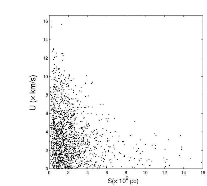
Figure 3: A plot of the $(S,U)$ pairs used in one Monte Carlo realization described in Section 5.1.

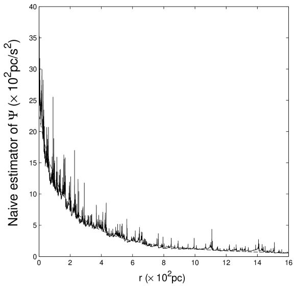
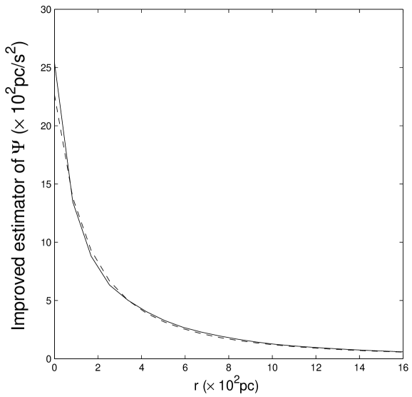
Figure 4: (Left) The ‘naive’ estimator $\Psi^{\#}$ as defined by Equation (18) and derived for the Monte-Carlo simulation described in Section 5.1 and for the $(S,U)$ pairs shown in Figure 3. (Right) The improved estimator $\hat{\Psi}$ derived from imposing the shape restrictions on the form of $M(r)$ (see Equations (20) and (21)) for the same simulated data set. In both figures the solid line is the estimator and the dashed line is the true distribution calculated from the underlying Plummer model.

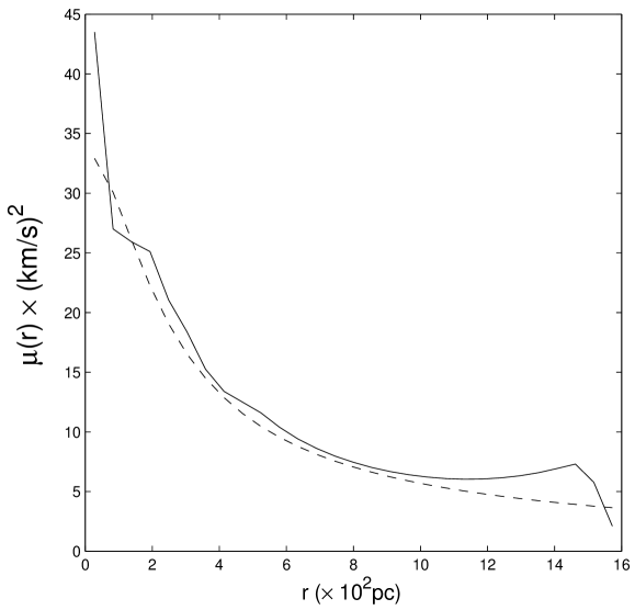
Figure 5: The radial velocity profile, $\mu(r)$, derived from the Monte-Carlo realization based on the Plummer Model described in Section 5.1. The actual profile calculated from the Plummer Model is shown as a dashed line. Our estimator, $\hat{\mu}(r)$ is shown as a solid line.

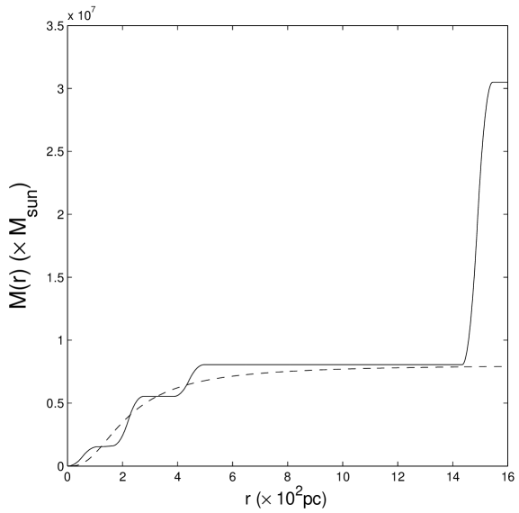
Figure 6: The estimator of the mass distribution, $\hat{M}(r)$ for the Monte-Carlo simulation based on a Plummer model described in Section 5.1. The piecewise nature of the estimator (see Equation (20) is apparent. The dashed line is the true mass distribution for the underlying Plummer model.

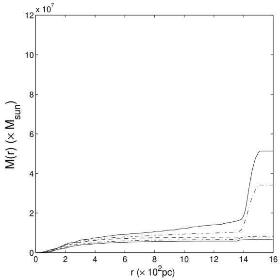
Figure 7: A plot of the 95% (solid lines) and 68% (inner dot-dashed lines) confidence bounds on the mass distribution, $M(r)$ (see Figure 6). The actual mass distribution from the Plummer model is shown as a dashed line. The strong positive bias at large $r$ (especially for $M(r)$) is evident for $r>14$ where the number of data points constraining the mass distribution is very low (about 1% of the entire sample lies outside $r\sim 14$).

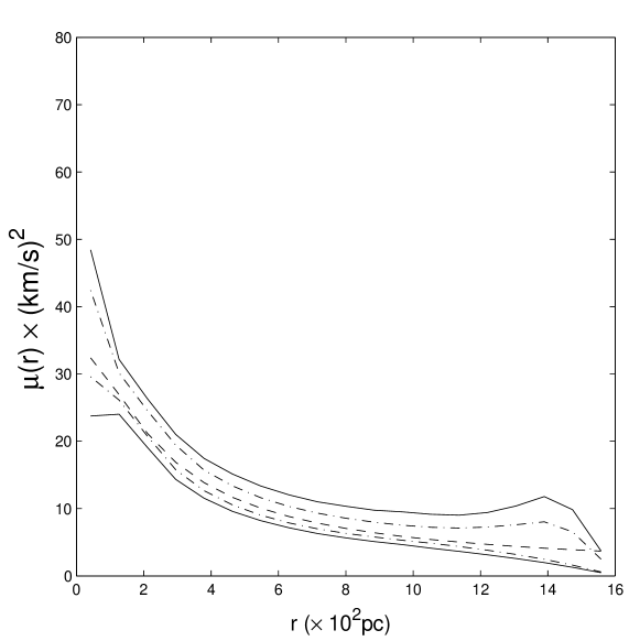
Figure 8: The 95% (solid lines) and 68% (dot-dashed lines) confidence bounds on the velocity dispersion profile estimator, $\hat{\mu}(r)$, along with the actual dispersion profile for the Plummer model (dashed line).

5 The Mass Profile: Simulations and a Trial Application

5.1 Monte-Carlo Simulations

To illustrate an application of our approach, we have drawn a sample of 1500 $(S,U)$ pairs from a Plummer model with $b=200\times 3.1\times 10^{15}\ km^{3}/sec^{2}$ and $\sigma_{i}^{2}=1$ (see Figure 3). The naive estimator $\Psi^{\#}$ may be computed from these data using Equation (18) and it is shown in Figure 4, along with the improved estimator $\hat{\Psi}$. The need for the improved estimator for $\Psi$ is clear since, as expected, $\Psi^{\#}$ is a highly irregular function which reacts strongly to the presence of individual data points. The estimated velocity dispersion profile, $\hat{\mu}(r)$ is presented in Figure 5 and the estimated mass profile, $\hat{M}(r)$, is illustrated in Figure 6. In all cases, the dotted line represents the true functions computed directly from the Plummer model from which the $(S,U)$ pairs were drawn. In these figures $n=1500$, $m=30$, and $w\equiv 1$.

The last plataux on the right in Figure 6 ($r>14$) deserves comments, because it illustrates an important feature of the problem in general and our method in particular: Estimates become unreliable for large values of $r$, because the data become sparse, and shape restricted methods are especially prone to problems such problems–e.g. Woodroofe and Sun (1993). Deciding exactly where reliability ends is difficult, but the confidence bands of Figures 7 and 9 provide some indication. In the example of Figure 6, they correctly predict that reliability deteriorates abruptly for $r>14$ and, interestingly, make the same prediction for a range of sample sizes.

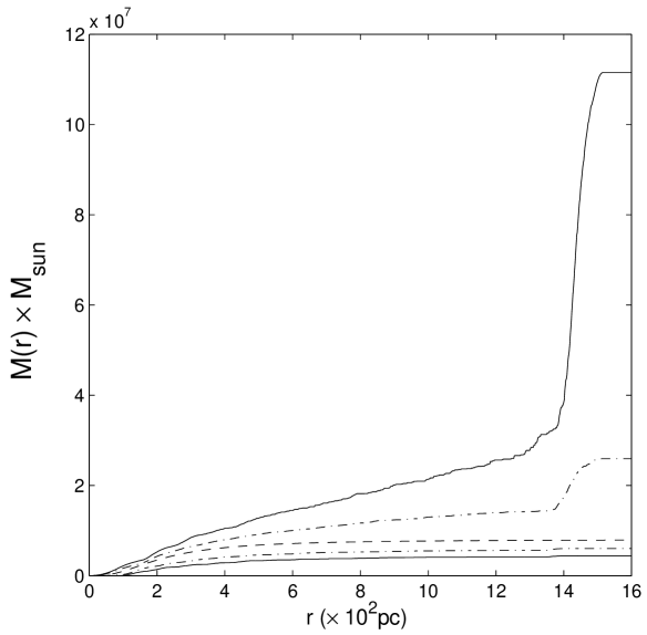
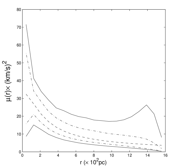
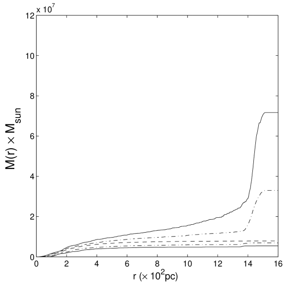
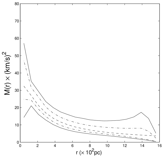
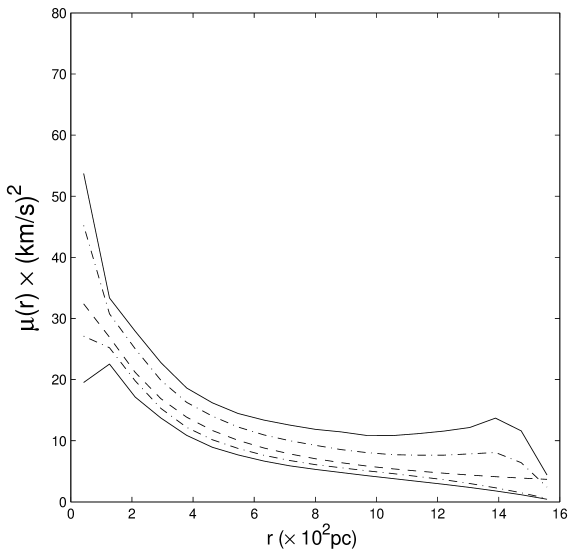
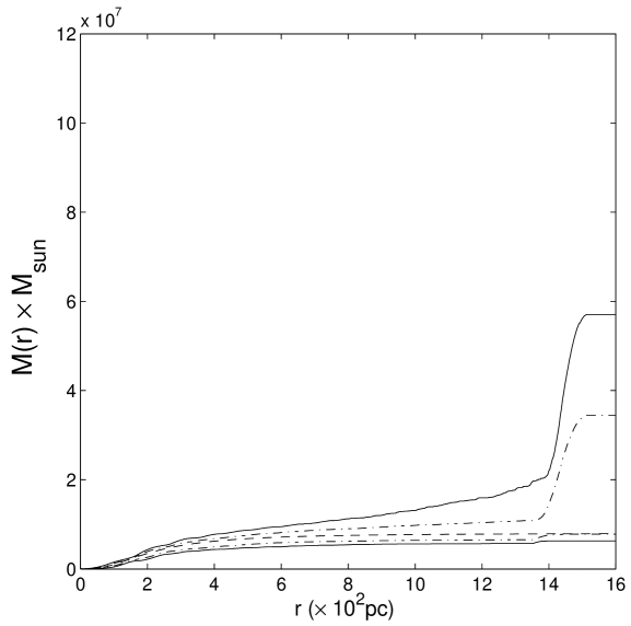
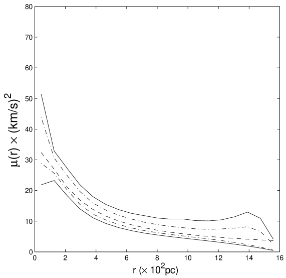
Figure 9: The $95\%$ (solid lines) and $68\%$ (dot-dashed lines) confidence bounds for different sample sizes of stars (from top, for 100, 400, 700 and 1000 stars) derived from a Plummer Model using Monte Carlo methods. The lefthand figures show the confidence bounds for the mass distribution estimator, $\hat{M}(r)$, and the righthand panels show the confidence bounds for the velocity dispersion profile estimator, $\hat{\mu}(r)$. In each panel, the dashed line is the true distribution for the Plummer model.

5.2 Assessing the Estimation Error

There are several sources of error in our derived velocity dispersion and mass profile estimators which may be divided into the broad classes of modeling error, systematic error, and statistical error. While quite general, our assumptions also represent some over-simplification and these too introduce uncertainty to our results. The assumption of spherical symmetry, for example, ignores the known ellipticities seen in most dSph galaxies (IH95, Mateo 1998). But even if we assume our working assumptions were all correct, systematic error will develop from our approximations of distributions as step functions, piecewise linear functions, and quadratic splines. On general grounds, this error will be small provided that the underlying true functions are smooth, so we feel justified in ignoring this source of systematic error. We have also ignored the statistical error in the estimation of $f$ in Section 3, because the sample sizes in IH95 are so large. That leaves the statistical error in the kinematic data as the principle source of uncertainty in our estimation of $\Psi$ and the estimators of $\mu$ and $M$.

To quantify the magnitude of this error, let $e(r)=\hat{M}(r)-M(r)$ denote the error committed when estimating $M(r)$, and let $z_{\alpha}(r)$ denote the $100\alpha^{th}$ percentile of its distribution distribution, so that $P[e(r)\leq z_{\alpha}(r)]=\alpha$. Then

$$P[\hat{M}(r)-z_{1-\alpha}(r)\leq M(r)\leq\hat{M}(r)-z_{\alpha}(r)]=1-2\alpha,$$

and $[\hat{M}(r)-z_{1-\alpha}(r),\hat{M}(r)-z_{\alpha}(r)]$ is a $100(1-2\alpha)$ percent confidence interval for $M(r)$. Within the context of Plummer’s Model, the $z_{\alpha}(r)$ can be obtained from a Monte Carlo simulation. If we generate $N_{MC}$ samples from Plummer’s Model, we obtain $N_{MC}$ values for the errors $e(r)$, which we denote as $e_{1}(r),\cdots,e_{N}(r)$. Then $z_{\alpha}(r)$ may be estimated by the value of $z$ for which the $N\alpha$ of the $e_{i}(r)$ are less than or equal to $z$. We applied this procedure to a grid of $r$ values with $N_{MC}=2000$ and $\alpha=0.025$ and then connected the resulting bounds to in a continuous piecewise linear fashion to obtain the 95% and 68% confidence bounds shown in Figure 7. The 95% and 68% confidence bounds for $\mu$ shown in Figure 8 were obtained in a similar manner.

The procedure just outlined requires knowing the true $M(r)$ and the distributions of $Y$ and $V_{3}$ from the Plummer model. But the exercise is still useful since it shows the intrinsic accuracy of the estimation procedure. For example, when the sample size is $1500$, the estimator of $M(r)$ has very little accuracy for $r\geq 14$. Somewhat surprisingly, the estimator for $M(r)$ retains reasonable accuracy for $r\leq 14$ despite the lack of much data beyond $r=14$ (see Figure 1). We have also explored how our estimates fare with significantly smaller samples of tracers with known positions and velocities (i.e., fewer $(S,U)$ pairs). Figure 9 shows $95$ percent confidence bounds for the estimates of $M(r)$ and $\mu(r)$ based on sample sizes $100$, $400$, $700$ and $1000$ stars. As one might expect, the confidence bounds expand as the sample size decreases, but, interestingly, the radial location of where the estimator performs poorly only very slowly migrates to smaller values of $r$ as the sample shrinks.

The requirement that we know $M(r)$ and the distribution of $Y$ and $V_{3}$ ahead of time in order to estimate the confidence bounds can be avoided by using a bootstrap procedure. In its simplest form, the bootstrap can be implemented as follows: Given a sample of $(Y,V_{3})$ values (corresponding to the observable projected position and radial velocity for each star in a kinematic sample), first compute $\hat{M}(r)$. Then generate $N_{b}$ samples with replacement from the given sample and compute estimators $\hat{M}_{1}^{*}(r),\cdots,\hat{M}_{N}^{*}(r)$ for each of these samples. Let $\hat{e}_{i}^{*}(r)=\hat{M}_{i}^{*}(r)-\hat{M}(r)$ and estimate the percentiles of $\hat{e}_{i}^{*}(r)$ as described above. Letting $\hat{z}_{\alpha}^{*}(r)$ denote the estimated $100\alpha^{th}$ percentile, $[\hat{M}(r)-\hat{z}_{1-\alpha}^{*}(r),\hat{M}(r)-\hat{z}_{\alpha}^{*}(r)]$ is the bootstrap confidence interval for $M(r)$. For more details, see Efrom and Tibshirani (1993) who provide a good introduction to bootstrap methods. This approach offers a practical way of assessing the statistical errors in $\hat{\mu}(r)$ and $\hat{M}(r)$ of an actual kinematic sample.

There is also the possibility of obtaining large-sample approximations to the error distribution. From (29), it is clear that the $z_{i}$ are approximately normally distributed in large samples. This suggests that the distribution of $\hat{\beta}$ should be approximately the same as the distribution of a shape-restricted estimator in a normal model. Unfortunately, calculating the latter is complicated. Some qualitative features are notable, however. Monotone regression estimators are generally quite reliable away from the end points, but subject to the spiking problem near the end points. For non-decreasing regression, the estimator has a positive bias near large values of the independent variable (in this case, $r$), and a negative bias at small values of the independent variable (i.e. for $r\sim 0$). The positive bias at large $r$ is very clearly seen in Figure 7 and is exacerbated by the sparsity of data. The negative bias near $r=0$ is not evident because it is ameliorated by two effects. First, the mass distribution is known to be always positive ($M(r)\geq 0$) and goes to zero at $r=0$ ($M(r=0)=0$). This eliminates bias at $r=0$. Second, our assumption (23) requires $\hat{M}(r)$ to be of order $r^{2}$ for small $r$, while $M(r)$ is – on physical grounds – known to approach zero as $r^{3}$ for small $r$.

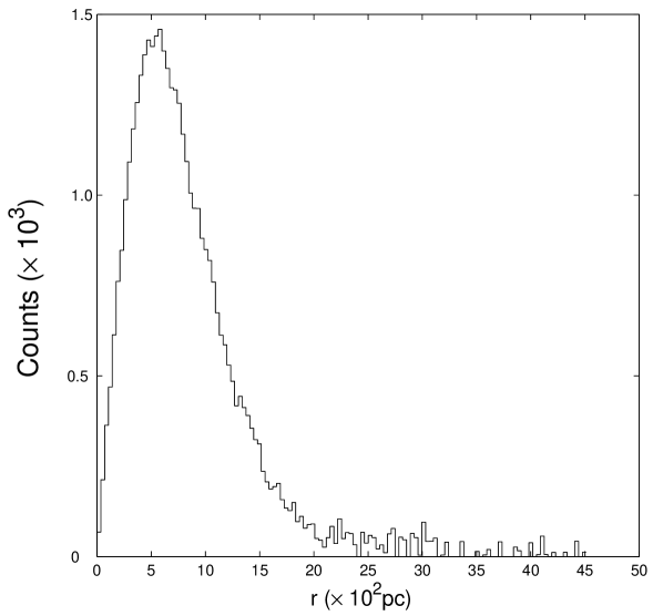
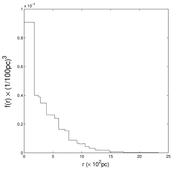
Figure 10: Observed and derived distributions from projected counts data in (Irwin and Hatzidimitriou, 1995). Top: Histogram of counts from IH95. Bottom: The inferred three-dimensional distribution of stars in Fornax assuming spherical symmetry, $\hat{f}(r)$; The projected radial distribution of stars in Fornax, $\hat{g}_{\bf Y}(y)$.

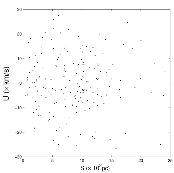
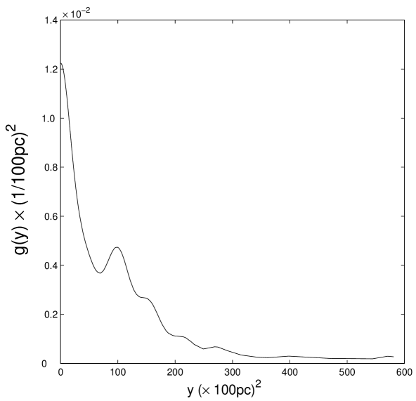
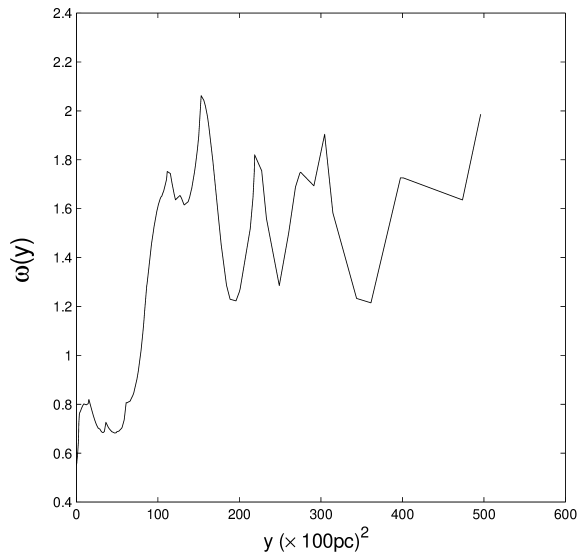
Figure 11: Observed and derived distributions from the kinematic dataset for the Fornax dSph galaxy (Walker et al. 2004). Top: The distribution of radial velocity/projected radial positions for the stars in the sample; Bottom: The projected radial distribution of stars in Fornax, $\hat{g}_{\bf Y}^{*}(y)$; The estimated selection function $\hat{\omega}$;

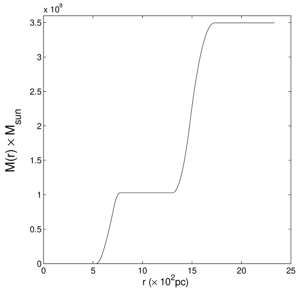
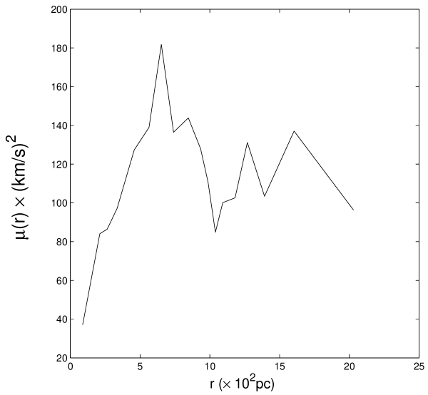
Figure 12: The mass distribution estimator for Fornax, $\hat{M}(r)$; The radial velocity dispersion profile estimator, $\hat{\mu}(r)$ of stars

5.3 Application of the Method: The Fornax Dwarf Spheroidal Galaxy

As an application to real observational data, we have use the radial velocity data from Walker et al (2005) for the Fornax dSph galaxy. This dataset consists of velocities for 181 stars observed one at a time over the past 12 years (Mateo et al. 1991 has a description of some of the earliest data used here). Data from newer multi-object instruments are not included here (see Walker et al 2005b for a first analysis of these newer results). Full details about the observations can be found in the papers referenced above; for the present application we simply adopt these results along with their quoted errors to see what sort of estimator for $M(r)$ we can extract from these data. From the simulations we already know that the dataset is relatively small for this method, but these simulations also imply that we have no reason to expect a strong bias in our mass estimator due to the sample size, only a potentially large uncertainty (at least a factor of 2) in the final mass estimate.

The histogram of the star counts from (Irwin and Hatzidimitriou 1995) is shown in the first panel of Figure 10. The remaining two panels in Figure 10 show the derived estimates for the spatial density of stars in Fornax $\hat{f}(r)$ and the true projected radial distribution of stars in Fornax $\hat{g}_{\bf Y}(y)$. The bottom panels of Figure 11 give the estimated projected radial distribution of stars from (Walker et al, 2004) and the estimated selection function $\omega(y)$ derived from the data. Figure 12 show the mass profile, $\hat{M}(r)$ and the squared velocity dispersion profile, $\hat{\mu}(r)$.

Previous estimates of the Fornax mass have been based primarily on the classical, or ’King’ (1966) analysis outlined in the introduction of this paper, and give $M_{Fornax}$ range from $6$ to $10\times 10^{7}$ M_⊙ (Mateo et al. 1991; Walker et al. 2005a). These models resemble truncated isothermal spheres and implicitly assume spherical symmetry, velocity isotropy, that mass follows light, and a specific parametric form for the joint density function $f_{0}(r,v)$. Our mass distribution estimator provides an independent measurement employing neither of the latter two assumptions. If one believes the second plateau seen at $r\geq 1.5$ kpc in Figure 12 (first panel) is a real feature, this would indicate a Fornax mass of $3.5\times 10^{8}M_{\odot}$. However, we note that the simulations using Plummer models (Figure 9) show similar plateaux at large radii related not to the underlying mass, but rather to the scarcity of remaining data points. The first plateau ($0.8<r<1.3$ kpc), by contrast, covers a region for which the Plummer simulations indicate even a relatively small dataset can yield a reasonable estimate of the mass. We therefore consider the two plateaux in the $M(r)$ curve of Figure 12 to bracket the region of plausible Fornax mass as measured from an N $\sim$ 200 sample by the estimation technique. The resulting interval of $1.0\times 10^{8}$M_⊙ $<$M_Fornax $<$ $3.5\times 10^{8}$ M_⊙ is of considerably larger mass than the results of the classical analysis.

The estimation approach then offers an attractive alternative to variants of the classical analysis that require parametric dynamical models to interpret kinematic data for dSphs. Our simulations show that this new non-parametric analysis will provide significantly more accurate results as kinematic samples grow larger.

Finally, we can make some comments regarding the effect of velocity anisotropy in our results. If we consider an extreme case where the outermost bins of the Fornax velocity dispersion profile are dominated by stars in tangential orbits (that is, $\overline{{v_{\theta}}^{2}}>>\overline{{v_{r}}^{2}}$; see Equations (1) and (2)), then the outer bins give us the mass directly (from Equation 1) as $M(r)\sim r\overline{{v_{\theta}}^{2}}/G$, or $10^{8}$ M_⊙, which is equivalent to the lower limit provided by the mass estimation technique. Thus, even if we consider an extreme breakdown of the isotropy assumption, the data alone support a larger mass than the simple King analysis. Since it is more likely that the velocity distribution has intermediate anisotropy (Kleyna et al. 2002), we conclude that the the mass of Fornax to the outermost measured data point is between $1.0$ and $3.5\times 10^{8}$ M_⊙ For an observed luminosity of $1.5\times 10^{7}$ L_⊙ for Fornax, this gives a global M/L ratio ranging from 7 to 22. Thus, even the most luminous, most baryonic-dominated dSph satellite of the Milky Way is dominated by dark matter.

6 Discussion

We have presented a new method for estimating the distribution of mass in a spherical galaxy. Along the way, we have made some choices, generally preferring the simplest of several alternatives–for example, the use of quadratic splines in Section 4 and simple histograms in Section 3. In spite of this, the algorithm is a bit complicated. Is it really better than simpler methods–for example, using kernel smoothing to estimate the distribution of projected radii and line of sight velocities and then using inversion to estimate $M(r)$? Our method differs from the simpler approach through its essential use of shape restrictions. From a purely statistical viewpoint, the monotonicity of $r^{3}\Psi^{\prime\prime}(r^{2})/f(r)$ in Equation (15) provides a lot of useful information [Robertson, et.al. (1988)]. Early in our investigations, we tried the kernel smoothing outlined above and found that the resulting estimators did not satisfy the shape restriction, leading to negative estimates of the mass density. Imposing the shape restrictions directly guarantees non-negative estimates, at least. It also reduces the importance of tuning parameters, like the bandwidth in kernel estimation or the number of bins in our work. Imposing the shape restrictions also complicates the algorithm and leaves a quadratic programming problem at the end. We think that the game is worth the candle.

There is some similarity between our method and that of Merritt and Saha (1993) in that both use basis functions, splines in our case, and both impose shape restrictions, the condition that $f>0$ in theirs. Our method makes more esssential use of shape restrictions and treats the inversion problem in greater detail.

This research was supported by grants from the National Science Foundation and the Horace Rackham Graduate School of the University of Michigan.

References

- (1) Binney, J., & Tremaine, S. 1987, Galactic Dynamics. Princeton Series in Astrophysics
- (2) Efrom, B, & Tibshirani, R. J. 1993,An Introduction to the Bootstrap, Chapman & Hall/CRC.
- (3) Gebhardt, K. & Fischer, P. 1995, AJ, 109, 209
- (4) Fleck, J.J., & Kuhn, J.R. 2003, ApJ, 592, 147
- (5) Groeneboon, P. & Jongbloed, K. 1995, Ann. Statist., 23, 1518
- (6) Gu, C. 2002, Smoothing Spline ANOVA Models. Springer.
- (7) Hall, P. & Smith, R. 1992, J. Comput. Phys., 74, 409
- (8) Hurley-Keller, D., Mateo, M., & Grebel, E. K. 1999, ApJ, 523, L25
- (9) Ibata, R.A., Gilmore, G., and Irwin, M.J. 1995, MNRAS, 277, 781.
- (10) Irwin, M., & Hatzidimitriou, D. 1995, MNRAS, 277, 1354
- (11) King, I.R. 1966, AJ, 71, 64
- (12) Klessen, R. S., Grebel, E. K., & Harbeck, D. 2003, ApJ, 589, 798
- (13) Klessen, R. S. & Kroupa, P. 1998, ApJ, 498, 143
- (14) Kleyna, J., Wilkinson, M. I., Evans, N. W., Gilmore, G., & Frayn, C. 2002, MNRAS, 330, 792
- (15) Kormendy, J., & Freeman, K. C. 2004, Dark Matter in Galaxies, IAU Symp. 220, eds. S. D. Ryder, D. J. Pisano & K. C. Freeman, p. 377
- (16) Kuhn, J. R. 1993, ApJ, 409, L13
- (17) Kuhn, J. R., Smith, H. A., & Hawley, S. L. 1996, ApJ, 469, L93
- (18) Kroupa, P. 1997, New Astronomy, 2, 139
- (19) Loader, C. 1999, Local Regression and Likelihood. Springer.
- (20) Majewski, S.R., Skrutskie, M.F., Weinberg, M.D., & Ostheimer, J.C. 2003, ApJ, 599, 1082
- (21) Mateo, M. 1998, ARAA, 36, 435
- (22) Mateo, M., Olszewski, E. W., Vogt, S. S., & Keane, M. J. 1998, AJ, 116, 2315
- (23) Mateo, M., Olszewski, E., Welch, D. L., Fischer, P., & Kunkel, W. 1991, AJ, 102, 914
- (24) Merritt, D., Meylan, G., & Mayor, M. 1997, AJ, 114, 1074
- (25) Merrit, D., Saha, P. 1993, ApJ, 409, 75
- (26) Oh, K.S., Lin, D.N.C., & Aarseth, S.J. 1995, ApJ, 442, 142
- (27) Pal, J. 2004, Shape restricted regression problems with applications to dark matter distributions. Thesis proposal, Statistics Department, The University of Michigan.
- (28) Piatek, S., & Pryor, C. 1995, AJ, 109, 1071
- (29) Richstone, D.O., & Tremaine, S. 1986, AJ, 92, 72R
- (30) Robertson, T., Wright, F. T., Dykstra, R. L. 1988, Order Restricted Statistical Inference. John Wiley & Sons Ltd.
- (31) Silverman, B. 1986, Density Estimation for Statistics and Data Analysis. Chapman & Hall.
- (32) Vogt, S. S., Mateo, M., Olszewski, E. W., & Keane, M. J. 1995, AJ, 109, 151
- (33) Walker, M.G., Mateo, M., Olszewski, E.W., Bernstein, R.A., Woodroofe, M., and Wang, X. 2005, submitted to AJ
- (34) Wicksell, S. D. 1925, Biometrika, 17, 84
- (35) Wilkinson, M.I., Kleyna, J., Evans, N.W., & Gilmore, G. 2002, MNRAS, 330, 778
- (36) Woodroofe, M., Sun, J. 1993, Statistica Sinica, 3, 501