Three-dimensional MHD simulations of X-ray emitting subcluster plasmas in cluster of galaxies

Abstract

Recent high resolution observations by the Chandra X-ray satellite revealed various substructures in hot X-ray emitting plasmas in cluster of galaxies. For example, Chandra revealed the existence of sharp discontinuities in the surface brightness at the leading edge of subclusters in merging clusters (e.g., Abell 3667), where the temperature drops sharply across the fronts. These sharp edges are called cold fronts. We present results of three-dimensional (3D) magnetohydrodynamic simulations of the interaction between a dense subcluster plasma and ambient magnetized intracluster medium. Anisotropic heat conduction along magnetic field lines is included. At the initial state, magnetic fields are assumed to be uniform and transverse to the motion of the dense subcluster. Since magnetic fields ahead of the subcluster slip toward the third direction in the 3D case, the strength of magnetic fields in this region can be reduced compared to that in the 2D case. Nevertheless, a cold front can be maintained because the magnetic field lines wrapping around the forehead of the subcluster suppress the heat conduction across them. On the other hand, when the magnetic field is absent, a cold front cannot be maintained because isotropic heat conduction from the hot ambient plasma rapidly heats the cold subcluster plasma.

, ,

1 Introduction

In recent years, high spatial resolution observations of clusters of galaxies by Chandra revealed the existence of sharp discontinuities of X-ray intensity called cold fronts (e.g., Markevitch et al., 2000; Vikhlinin et al., 2001b). Their existence is challenging because in high temperature plasma, high thermal conductivity quickly smears such a discontinuity in temperature. Ettori and Fabian (2000) pointed out that heat conductivity across the front should be reduced from the classical Spitzer value, $\kappa_{\rm Sp}=5\times 10^{-7}T^{5/2}\,{\rm erg\,s^{-1}\,cm^{-1}\,K^{-1}}$ (Spitzer, 1962) by several orders of magnitude. Magnetic fields enable such suppression. Cold fronts may also be subject to the Kelvin-Helmholtz (K-H) instability. Vikhlinin et al. (2001a, b) suggested that turbulent magnetic fields stretched along the cold front will reduce the growth rate of the K-H instability at the interface between a subcluster plasma and an ambient plasma.

The magnetic field strength in the core of clusters of galaxies can be the order of ${\rm\mu G}$ (e.g., Kronberg, 1994; Carilli and Taylor, 2002). Johnston-Hollitt (2004) summarized the observations of the field strength in several regions of Abell 3667 by using different techniques. They showed that its strength in the cluster core is about $1-2\,{\rm\mu G}$, and that magnetic fields are tangled on scales of roughly $100\,{\rm kpc}$.

Let us estimate the heat conduction time scale in cluster of galaxies. It has been suggested that the heat conduction in cluster of galaxies can be very efficient (e.g., Takahara and Ikeuchi, 1977) because the Coulomb mean free path, $l_{\rm c}\sim 5\,(kT/5\,{\rm keV})^{2}(n/10^{-3}\,{\rm cm^{-3}})^{-1}\,{\rm kpc}$, is large. Here, $n$ is the number density. The time required for heat to diffuse by conduction across a length $L$ is given by $\tau_{\rm Sp}\sim\rho L^{2}/\kappa_{\rm Sp}\sim 3\times 10^{7}(kT/5\,{\rm keV})^{-5/2}(n/10^{-3}\,{\rm cm^{-3}})(L/100\,{\rm kpc})^{2}\,{\rm yr}$, where $\rho$ is the density and $\kappa_{\rm Sp}$ is the Spitzer conductivity. Since the thickness of the cold front is much smaller than $100\,{\rm kpc}$, they will disappear in a time scale shorter than $10^{7}\,{\rm yr}$. If magnetic fields exist, however, the characteristic length of the heat exchange across magnetic field lines is reduced to the Larmor radius, $r_{\rm L}=2500\,(B/1\,{\rm\mu G})^{-1}(kT/5\,{\rm keV})^{1/2}\,{\rm km}$. Thus, the heat conduction across the magnetic field is almost suppressed.

Earlier numerical studies of cold fronts (e.g., Heinz et al., 2003) did not include magnetic fields and heat conduction. Asai et al. (2004) first reported the results of two-dimensional (2D) magnetohydrodynamic (MHD) simulations of cold fronts including both magnetic fields and anisotropic heat conduction. They showed that magnetic fields are stretched and elongated ahead of the front. Since these magnetic fields suppress the heat conduction across them, the contact discontinuity (a cold front) between the cold subcluster plasma and the hot ambient plasma can be maintained. The cold subcluster is wrapped by magnetic fields and protected from being heated by the heat conduction.

In this paper, we focus on the three-dimensional (3D) effects. In the 3D case, since magnetic fields compressed in front of the cold front can expand in the third direction or slip out the front surface, the strength of the magnetic fields in this region may be reduced compared to that in the 2D case. We would like to show that even when we include these 3D effects, cold fronts can be maintained.

2 Simulation model

We simulated the time evolution of a cluster plasma in a frame comoving with the subcluster. The basic equations are as follows:

$$\frac{\partial\rho}{\partial t}+\mbox{\boldmath$\nabla$ $\cdot$}(\rho\mbox{\boldmath$v$})=0,$$ (1)

$$\rho\left[\frac{\partial\mbox{\boldmath$v$}}{\partial t}+(\mbox{\boldmath$v$ $\cdot$ $\nabla$})\mbox{\boldmath$v$}\right]=-\mbox{\boldmath$\nabla$}{\it p}+\frac{(\mbox{\boldmath$\nabla$}\times\mbox{\boldmath$B$})\times\mbox{\boldmath$B$}}{4\pi}-\rho\mbox{\boldmath$\nabla$}\psi,$$ (2)

$$\frac{\partial\mbox{\boldmath$B$}}{\partial t}=\mbox{\boldmath$\nabla$}\times(\mbox{\boldmath$v$}\times\mbox{\boldmath$B$}),$$ (3)

$$\frac{\partial}{\partial t}\left[\frac{1}{2}\rho v^{2}+\frac{B^{2}}{8\pi}+\frac{p}{\gamma-1}\right]$$

$$+\mbox{\boldmath$\nabla$$\cdot$}\left[\left(\frac{1}{2}\rho v^{2}+\frac{\gamma p}{\gamma-1}\right)\mbox{\boldmath$v$}+\frac{1}{4\pi}(-\mbox{\boldmath$v$}\times\mbox{\boldmath$B$})\times\mbox{\boldmath$B$}-\kappa_{\parallel}\mbox{\boldmath$\nabla_{\parallel}$}T\right]=-\rho\mbox{\boldmath$v$ $\cdot$ $\nabla$}\psi,$$

where $\rho$, $v$, $p$, $B$, and $\psi$ are the density, velocity, pressure, magnetic fields, and gravitational potential, respectively. We use the specific heat ratio $\gamma=5/3$. The subscript $\parallel$ denotes the components parallel to the magnetic field lines. We assume that heat is conducted only along the field lines. We solved ideal MHD equations in a Cartesian coordinate system $(x,y,z)$ by a modified Lax-Wendroff method with artificial viscosity. The heat conduction term in the energy equation is solved by the implicit red and black successive overrelaxation method (see Yokoyama and Shibata, 2001, for detail). The radiative cooling term is not included. The units of length, velocity, density, pressure, temperature, and time in our simulations are $r_{0}=250\,{\rm kpc}$, $v_{0}=800\,{\rm km\,s^{-1}}$, $\rho_{0}=5\times 10^{-27}\,{\rm g\,cm^{-3}}$, $p_{0}=3\times 10^{-11}\,{\rm erg\,cm^{-3}}$, $kT_{0}=4\,{\rm keV}$, and $t_{{0}}=r_{0}/v_{0}=3\times 10^{8}\,{\rm yr}$, respectively.

Figure 1 shows the initial density distribution. Solid lines and arrows show magnetic field lines and velocity vectors in the $y=0$ plane, respectively. We assume that a spherical isothermal low-temperature ($kT_{\rm in}=4\,{\rm keV}$) plasma is confined by the gravitational potential of a subcluster. The low-temperature plasma is embedded in the less-dense $(\rho_{\rm out}=0.25\,\rho_{0})$ uniform, hot $(kT_{\rm out}=8\,{\rm keV})$ plasma. Here the subscripts “in” and “out” denote the values inside and outside the subcluster, respectively.

We assume that the density distribution of the subcluster is given by the $\beta$-model profile (Cavaliere and Fusco-Femiano, 1976),

$$\rho_{\rm in}=\rho_{\rm c}\left[1+\left(\frac{r}{r_{\rm c}}\right)^{2}\right]^{-3\beta/2}$$ (5)

where $r=(x^{2}+y^{2}+z^{2})^{1/2}$, $\beta=2/3$, the maximum density $\rho_{\rm c}=10^{-26}\,{\rm g\,cm^{-3}}$, and the core radius is $r_{\rm c}=290\,{\rm kpc}$. The subcluster is initially in hydrostatic equilibrium under the gravitational potential fixed throughout the simulation.

We assume that ambient plasma initially has a uniform speed with Mach number $M=v_{x}/c_{\rm s\,out}=1$, where $c_{\rm s\,out}$ is the ambient sound speed. The Mach number with respect to the sound velocity inside the subcluster is $M^{\prime}=v_{x}/c_{\rm s\,in}=\sqrt{2}$.

Table 1 shows model parameters. An important parameter is the plasma beta ($\beta_{0}$) defined as the ratio of the ambient gas pressure to the magnetic pressure. When $\beta_{0}=p_{\rm gas}/p_{\rm mag}=100$, the magnetic field strength is $B\sim 1.5\,{\rm\mu G}$. Models HC2 (2D) and HC3 (3D) are non-magnetic models with isotropic heat conduction, and model MC2a (2D) and MC3a (3D) are models with magnetic fields ($\beta_{0}=100$) and anisotropic heat conduction. Model MC2b (2D) is a model with weak magnetic fields ($\beta_{0}=1000,B\sim 0.5\,{\rm\mu G}$) and anisotropic heat conduction. Model MC3b (3D) is a model with weaker magnetic fields ($\beta_{0}=10^{3},B\sim 0.15\,{\rm\mu G}$). We note that the initial magnetic fields are parallel to the $z$-axis and perpendicular to the motion of the subcluster.

When magnetic fields exist, heat is conducted only in the direction parallel to the field lines. Along the magnetic fields, the heat conductivity is taken to be that of the Spitzer conductivity, $\kappa_{\parallel}=5\times 10^{-7}\,T^{5/2}\,{\rm erg\,s^{-1}\,cm^{-1}\,K^{-1}}$. Meanwhile the conductivity across the field lines is $\kappa_{\perp}=0$. The conduction time scale along the field lines is $\tau_{\kappa}\sim\rho L^{2}/\kappa_{\parallel}\sim 3\times 10^{7}\,(kT/5\,{\rm keV})^{-5/2}(n/10^{-3}\,{\rm cm^{-3}})\\ (L/100\,{\rm kpc})^{2}\,{\rm yr}$.

For boundary conditions, the left boundary at $x=-5$ is taken to be a fixed boundary, and other boundaries are taken to be free boundaries where waves can be transmitted.

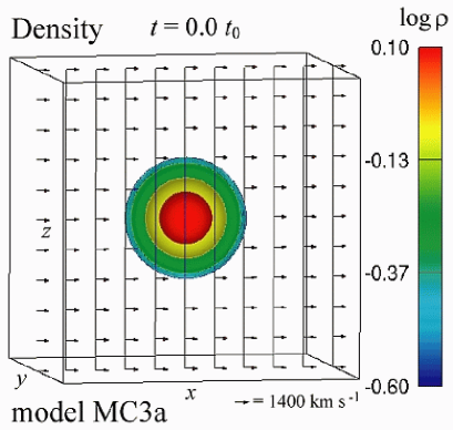
Figure 1: Initial density distribution visualized as logarithm of the density.

Table 1: Models and parameters. Heat conduction is isotropic in models HC2 and HC3. In other models, heat conducts only along magnetic fields.

Model	$\beta_{0}$	$\kappa$	$kT_{\rm in}$[keV]	$kT_{\rm out}$[keV]	simulation box	number of grid points
HC2	$\infty$	$\kappa$	4	8	${(2.5{\rm Mpc})}^{2}$	$1200^{2}$
MC2a	100	$\kappa_{\parallel}$	4	8	${(2.5{\rm Mpc})}^{2}$	$1200^{2}$
MC2b	1000	$\kappa_{\parallel}$	4	8	${(2.5{\rm Mpc})}^{2}$	$1200^{2}$
HC3	$\infty$	$\kappa$	4	8	${(2.5{\rm Mpc})}^{3}$	$280^{3}$
MC3a	100	$\kappa_{\parallel}$	4	8	${(2.5{\rm Mpc})}^{3}$	$280^{3}$
MC3b	$10^{4}$	$\kappa_{\parallel}$	4	8	${(2.5{\rm Mpc})}^{3}$	$280^{3}$

3 Results

3.1 Configuration of magnetic fields

Figure 2 shows the magnetic fields for model MC3a at $t=1\,{\rm Gyr}$. Solid curves and color contours show the magnetic field lines and density distribution, respectively. The subcluster plasma is wrapped by the magnetic field lines. Ahead of the subcluster, the magnetic field lines are almost parallel to the contact surface between the subcluster plasma and the ambient plasma. We can identify magnetic field lines slipping in the $y$-direction.

Figure 3 shows isocontours of magnetic field strength in the $y=0$ plane for models MC3a (left, 3D) and MC2a (right, 2D) at $t=1\,{\rm Gyr}$, respectively. Arrows show velocity vectors. We note that the initial magnetic field lines are parallel to the $z$-axis. The magnetic field strength is enhanced ahead of the subcluster via compression. Compared to the 2D model (right), magnetic fields in the 3D model are weaker ahead of the subcluster but their strength is enhanced at the tail of the subcluster because the plasma flows advect the magnetic fields toward the tail and they pile up in the tail.

The left panel of Figure 4 shows the distribution of magnetic field strength at $t=1\,{\rm Gyr}$ along the $x$-axis. The solid curve shows their strength for model MC3a (3D, $\beta_{0}=100$). The dotted line and the long-dashed line show their strength for model MC2a (2D, $\beta_{0}=100$) and MC2b (2D, $\beta_{0}=1000$), respectively. Their strength in front of the cold front is enhanced more than a factor 3 from the initial state. The right panel in Figure 4 shows the time evolution of the total magnetic energy integrated in the whole simulation region. The magnetic energy increases gradually due to magnetic field compression around the subcluster.

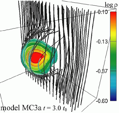
Figure 2: Magnetic field lines at $t=1\,{\rm Gyr}$. Color contours show the logarithmic density distribution. The solid curves show magnetic field lines.

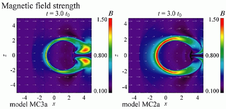
Figure 3: Comparison of the magnetic field strength at $t=1\,{\rm Gyr}$ between 3D (left) and 2D (right). The left and right panels show the result for models MC3a and MC2a at $y=0$ plane, respectively. Arrows show the velocity vectors.

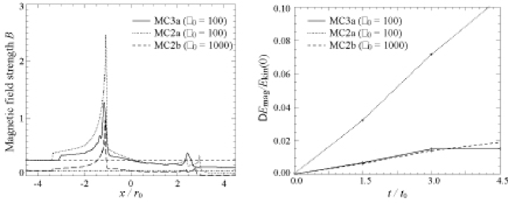
Figure 4: Left: Distributions of magnetic field strength at $t=1\,{\rm Gyr}$. The solid curve shows magnetic field strength for model MC3a (3D, $\beta_{0}=100$) along the $x$-axis. The dotted curve and the long-dashed curve show the strength for model MC2a (2D, $\beta_{0}=100$) and MC2b (2D, $\beta_{0}=1000$) along the $x$-axis, respectively. The dashed line and dash-dotted line show the initial magnetic field strength for models with $\beta_{0}=100$ and $\beta_{0}=1000$, respectively. Right: Time evolution of the magnetic energy ($E_{\rm mag}$) integrated in the whole simulation region. The increase with respect to the initial kinetic energy, $\Delta E_{\rm mag}/E_{\rm kin}(0)=(E_{\rm mag}(t)-E_{\rm mag}(0))/E_{\rm kin}(0)$, is plotted. The solid line, dotted line, and long-dashed line are for models MC3a (3D, $\beta_{0}=100$), MC2a (2D, $\beta_{0}=100$), and MC2b (2D, $\beta_{0}=1000$), respectively.

3.2 Effects of magnetic fields on heat conduction

Let us compare the results for model MC3a (with heat conduction) and model HC3 (without heat conduction). We show in Figure 5 distributions of the projected density, temperature, and X-ray intensity obtained by integrating these quantities in the $y$-direction. X-ray intensity are visualized from simulation results as logarithm of the thermal bremsstrahlung emissivity, $\sim\rho^{2}$. In model HC3 (lower panels), heat is conducted isotropically. Since the conduction time scale across the cold front with width $\sim 5{\rm kpc}$ (Vikhlinin et al., 2001b) is very short ($\tau_{\kappa}\sim 10^{7}{\rm yr}$), the cool component inside the subcluster is heated by the hot ambient plasma and evaporates rapidly. Meanwhile in model MC3a (top panels), heat is conducted only in the direction parallel to the field lines. As we showed in §3.1, since the subcluster is wrapped by magnetic field lines, the cool component inside the subcluster is protected from heating. We can see this protection remarkably in the temperature distributions (middle panels). Thus the discontinuity remains sharp.

Figure 6 shows the temperature profiles at $t=1{\rm Gyr}$ along the $x$-axis. The left panel shows those for models MC3a (solid line) and HC3 (dotted line). The right panel shows those for models MC2a (solid line), MC2b (dash-dotted line), and HC2 (dotted line). In both panels, the dashed line shows the initial temperature profile. It is obvious that magnetic fields along the front enables the cold front to exist for $1{\rm Gyr}$.

We can also identify shock waves. Numerical results reproduced the bow shock produced by supersonic motion upstream of the cold front observed in A3667 (see Figure 5). The interaction of the subcluster plasma with the ambient plasma generates another shock propageting inside the subcluster. This shock exists at $x=2.5$ in models MC3a and MC2a (solid lines) in Figure 6, and also visible in the left panel of Figure 4. These shocks drive the adiabatic expansion of the subcluster and cools the subcluster plasma. Such behaviors are consistent with those in 2D models (Asai et al., 2004).

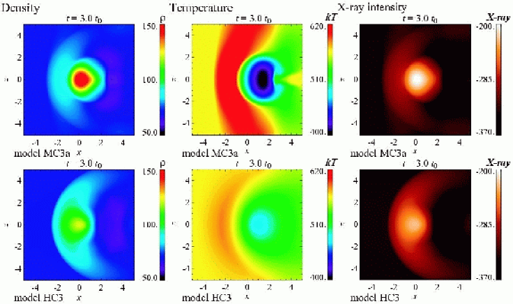
Figure 5: Distribution of projected density (left), temperature (middle), and X-ray intensity (right) integrated at $t=1{\rm Gyr}$ along the $y$-axis. The top panels show results for model MC3a (with magnetic fields and heat conduction). The bottom panels show results for model HC3 (without magnetic fields and with heat conduction).

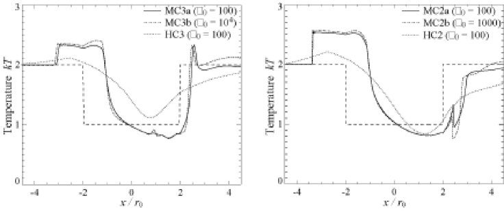
Figure 6: Comparison of the temperature distributions between 3D (left) and 2D (right) at $t=1\,{\rm Gyr}$ along the $x$-axis. The left panel shows the results for models MC3a (solid line), MC3b (dash-dotted line), and HC3 (dotted line). The right panel shows the results for models MC2a (solid line), MC2b (dash-dotted line), and HC2 (dotted line). The dashed lines in both panels show the initial temperature distribution.

4 Discussion

4.1 Importance of magnetic fields for the existence of cold fronts

We have shown that magnetic fields enable the existence of cold fronts by suppressing the heat conduction across the front. Previous hydrodynamic simulations (e.g., Heinz et al., 2003) could reproduce the cold fronts because they neglected the heat conduction. When heat conduction is included, cold fronts disappear in time scales of $\sim 10^{8}\,{\rm yr}$ unless the heat conduction is suppressed as we showed in models HC2 and HC3 (see Figures 5 and 6). Magnetic fields much smaller than that in model MC3a can suppress heat conduction. We confirmed that weak magnetic fields for model MC3b ($\beta_{0}=10^{4},B\sim 0.15\,{\rm\mu G}$) can suppress the heat conduction across the front as long as they cover the front. Even when large-scale coherent magnetic fields do not exist, turbulent magnetic fields can suppress the heat conduction across the front; they are stretched and elongated parallel to the front (see also Vikhlinin et al., 2001a; Asai et al., 2004).

Vikhlinin et al. (2001a, b) suggested that magnetic fields are important for the existence of cold fronts because they can suppress the growth of the K-H instability. Asai et al. (2004) showed that in models without heat conduction and without magnetic fields, the growth of the K-H instability is not prominent and does not disrupt the cold front ahead of the moving subcluster. In the sides of the subcluster, the K-H instability creates eddies which detach and propagate downstream. Magnetic fields can suppress the formation of such eddies.

4.2 Possibility of subcluster disruption by magnetic fields accumulating ahead of the subcluster

Let us now discuss the possibility of the disruption of the subcluster plasma by magnetic fields. Gregori et al. (2000) presented the results of 3D simulations of moderate supersonic cloud motion in a magnetized interstellar medium. They assumed that the cloud has uniform density. They showed that magnetic fields accumulating ahead of the cloud triggers the Rayleigh-Taylor (R-T) instability and disrupts the cloud. Our numerical results, however, does not show the growth of such R-T instability. These different behaviors are due to a difference of the density distribution of the cloud. Since the subcluster plasma in our simulations has a dense core because it is confined by the gravity, magnetic fields ahead of the clump can not deform the density distribution inside the subcluster.

4.3 Three-dimensional effects

We have shown that in the 3D case, since magnetic fields ahead of the subcluster slip along the contact surface between the subcluster plasma and the ambient plasma, the amplification of their strength is smaller than that in the 2D case. This weaker magnetic field, however, is sufficient to suppress the heat conduction across the front.

Since the area of the contact surface is larger in the 3D case than that in the 2D case. Thus cold subcluster plasma can be heated more efficiently than in the 2D case. We confirmed this by comparing results for model HC2 and HC3 (Figure 6). Compared with model HC2 (2D, non-magnetic fields), the temperature profile for model HC3 (3D, non-magnetic fields) shows that the cold subcluster is heated up earlier. When magnetic fields exist, however, the difference becomes less prominent.

References

- Asai et al. (2004) N. Asai, N. Fukuda and R. Matsumoto, Magnetohydrodynamic simulations of the formation of cold fronts in clusters of galaxies including heat conduction, ApJ 606 (2004), pp. L105-L108.
- Carilli and Taylor (2002) C. L. Carilli and G. B. Taylor, Cluster magnetic fields, ARA&A 40 (2002), pp. 319-348.
- Cavaliere and Fusco-Femiano (1976) A. Cavaliere and R. Fesco-Femiano, X-rays from hot plasma in clusters of galaxies, A&A 49 (1976), pp. 137-144.
- Ettori and Fabian (2000) S. Ettori and A. C. Fabian, Chandra constraints on the thermal conduction in the intracluster plasma of A2142, MNRAS 317 (2000), pp. L57-L59.
- Gregori et al. (2000) G. Gregori, F. Miniati, D. Ryu and T. W. Jones, Three-dimensional magnetohydrodynamic numerical simulations of cloud-wind interactions, ApJ 543 (2000), pp. 775-786.
- Heinz et al. (2003) S. Heinz, E. Churazov, W. Forman, C. Jones and U. G. Briel, Ram pressure stripping and the formation of cold fronts, MNRAS 346 (2003), pp. 13-17.
- Johnston-Hollitt (2004) M. Johnston-Hollitt, The magnetic field in A3667, in: T. H. Reiprich, J. C. Kempner, N. Soker, (Eds.), The Riddle of Cooling Flows in Galaxies and Clusters of Galaxies, URL: http://www.astro.virginia.edu/coolflow/, (2004).
- Kronberg (1994) P. P. Kronberg, Extragalactic magnetic fields, Rep. Prog. Phys. 57 (1994), pp. 325-382.
- Markevitch et al. (2000) M. Markevitch, T. J. Ponman and P. E. J. Nulsen, et al., Chandra observation of Abell 2142: Survival of dense subcluster cores in a merger, ApJ 541 (2000), pp. 542-549.
- Spitzer (1962) L. Spitzer, Physics of Fully Ionized Gases, New York: Interscience (2nd edition), (1962).
- Takahara and Ikeuchi (1977) F. Takahara, and S. Ikeuchi, On the origin and evolution of the intracluster gas —Interaction with galaxies—, Prog. Theor. Phys., 58 (1977), pp. 1728-1741.
- Vikhlinin et al. (2001a) A. Vikhlinin, M. Markevitch and S. S. Murray, Chandra estimate of the magnetic field strength near the cold front in A3667, ApJ 549 (2001a), pp. L47-L50.
- Vikhlinin et al. (2001b) A. Vikhlinin, M. Markevitch and S. S. Murray, A moving cold front in the intergalactic medium of A3667, ApJ 551 (2001b), pp. 160-171.
- Yokoyama and Shibata (2001) T. Yokoyama, and K. Shibata, Magnetohydrodynamic simulation of a solar flare with chromospheric evaporation effect based on the magnetic reconnection model, ApJ 549 (2001), pp. 1160-1174.