A Multi-Instrument Study of the Helix Nebula Knots with the Hubble Space Telescope

Abstract

We have conducted a combined observational and theoretical investigation of the ubiquitous knots in the Helix Nebula (NGC 7293). We have constructed a combined hydrodynamic+radiation model for the ionized portion of these knots and have accurately calculated a static model for their molecular regions. Imaging observations in optical emission lines were made with the Hubble Space Telescope’s STIS spectrograph, operating in a “slitless” mode, complemented by WFPC2 images in several of the same lines. The NICMOS camera was used to image the knots in H₂. These observations, when combined with other studies of H₂ and CO provide a complete characterization of the knots. They possess dense molecular cores of densities about 10⁶ cm^-3 surrounded on the central star side by a zone of hot H₂. The temperature of the H₂ emitting layer defies explanation either through detailed calculations for radiative equilibrium or for simplistic calculations for shock excitation. Further away from the core is the ionized zone, whose peculiar distribution of emission lines is explained by the expansion effects of material flowing through this region. The shadowed region behind the core is the source of most of the CO emission from the knot and is of the low temperature expected for a radiatively heated molecular region.

1. INTRODUCTION

A pressing issue within the study of the planetary nebulae (PN) is the nature of the highly compact, neutral core knots that have been found in all the nearby PN studied by the Hubble Space Telescope (HST) and arguably are ubiquitous (O’Dell et al. 2002, henceforth O2002). Their origin is not established, although two extreme models exist, the first, where they originate as knots in the extended atmosphere of the precursor central star (Dyson et al. 1989, Hartquist & Dyson 1997) and the second possibility is that they are the results of instabilities occurring at the boundary between the ionized and neutral zones within the nebulae (Capriotti 1973). Perhaps the most significant issue about them is not their origin, rather “What is their fate?” This is because their survival beyond the PN stage would mean that a large fraction of the material being put into the interstellar medium (ISM) by the PN phenomenon would be trapped in optically thick knots, which would then become a new component of the ISM. However, to delve into their origin or prognosticate their future, we must understand the objects as they are now. Fortunately, these knots have become the subjects of recent observational studies that probe from the outside to the inside of the knots and we can begin to hope of having a complete picture of their nature. This paper presents new observational results for the nearest bright PN, NGC 7293–the Helix Nebula, that probe both the outer ionized layers and a portion of the neutral inner core of its knots. These observations are then compared with new sophisticated models that accurately model the regions of origin of the emission and we present a general model for the objects.

The Helix Nebula is a member of the polypolar class of PN where there is a smaller filled inner-disk within a fainter outer-disk that is almost perpendicular to it (O’Dell, et al. 2004, henceforth OMM2004). The outer-disk is open in the middle where it encloses the inner-disk and its opening is surrounded by a brighter feature called the outer-ring. Both are optically thick to ionizing Lyman continuum (LyC) radiation. The innermost portions of the inner-disk contains a core of He⁺⁺ emission, whose lack of ions with high emissivity give the nebula a superficial appearance of having a central cavity (O’Dell 1998, henceforth O1998). The several thousand knots that are present in the Helix Nebula begin to be seen about about the region of transition from He⁺⁺ to He⁺ and they are found with increasing concentration as one moves toward the ionization boundary, both in the inner-disk and the outer-ring (OMM2004).

The knots were originally discovered by Walter Baade and first reported upon by Zanstra (1955) and Vorontzov-Velyaminov (1968). The next big step in the illumination of the knots was the paper by Meaburn et al. 1992 (henceforth M1992), which established that the knots had highly ionized cusps of about 2″ size facing the hot central star, little emission in the [O III] emission line, and that the dust in their central cores blocked out some of the background nebular emission, the amount of this extinction providing information about their location within the nebula. This picture was extended by much higher spatial resolution images made with the HST, which has now covered several portions of the nebula in the northern quadrant (O’Dell & Handron 1996, henceforth OH1996, O’Dell & Burkert 1997, henceforth OB1997) and with lower signal to noise ratio, a section in the main ring of emission to the northwest from the central star (O2002). There are about 3,500 knots in the entire nebulae (OH1996) and the characteristic mass of each is about 3 x 10^-5 M_sun (OB1997) or $\gtrsim$ 1 x 10^-5 M_sun (Huggins et al. 2002, henceforth H2002), the former value meaning that the knots contain a total mass of about 0.1 M_sun, which is about the same as all of the ionized gas. This indicates that the knots represent an important ingredient in the mass-loss process of this PN. The HST Wide Field and Planetary Camera 2 (WFPC2) allowed distinguishing between the low ionization [N II] emission and that of H$\alpha$ and [O III]. This information, together with slitless spectra (O’Dell, et al. 2000, henceforth OHB2000) established that the ionization structure of the bright knots was dissimilar to other photoionized structures in that the [N II] structure is more diffuse than that in H$\alpha$, which could be explained by the rather ad hoc introduction of a peculiar electron temperature distribution, which is now explained by the dynamical model introduced in this paper. The inner knots show well defined “tails” which has led to the knots sometimes being called “cometary knots”. The radial alignment of these features has suggested to some authors that there may be a radial outflow of material along them (Dyson, Hartquist, & Biro 1993), although the shadowing of ionizing Lyman Continuum radiation must play an important role (Cantó et al. 1998, O’Dell 2000).

The regions within the bright ionized cusps have been probed by observations of their molecular cores which now have sufficient resolution to make a clear delineation of the emission as arising from the core of the knots, rather than an extended Photon Dominated Region (PDR) lying outside the ionization front of the nebula. The entire Helix Nebula has been imaged (Speck et al. 2002, henceforth S2002) in the H₂ 2.12 µm line at a resolution of about 2″. This study is supplemented by a 1.2″ resolution image of one of the knots by H2002. Radio observations in other molecules have been of progressively better spatial resolution, with the entire nebula having now been mapped at 31″ in CO by Young et al. 1999 (henceforth Y1999) where the presence of multiple velocity components within the beam indicate that there were emitting regions smaller than the beam size. H2002 made CO observations with an elliptical beam of 7.9″x 3.8″ of the same knot as in their high resolution H₂ study. A splendid spectroscopic study at 6″ spatial resolution of multiple H₂ emission lines established (Cox et al. 1998) that the H₂ levels are in statistical equilibrium and that the temperature of the H₂ portions of the cores is a surprising 900K. The best resolution study of neutral hydrogen is that of Rodríguez, Goss, & Williams (2002) , although their 54.3″x 39.3″ beam was insufficient to distinguish between emission coming from within the knots or the PDR associated with the nebula’s ionization front.

Fortunately, we know a lot of the basic characteristics of the system. The trigonometric parallax of Harris et al. (1997) indicates that the distance is 213 parsecs, which means that 1″ = 3.19 x 10¹⁵ cm and the 500″ semimajor axis of the inner-disk (OMM2004) corresponds to 0.52 pc. The dynamic age of the inner-disk is 6,600 years (OMM2004). The central star has been measured accurately in the Far Ultra Violet (FUV, the ultraviolet flux with frequences below the Lyman limit) by Bohlin et al. (1982), who found an effective temperature of 123,000 K. At 213 pc distance the star must have a bolometric luminosity of 120 L_sun. The central region has also been measured in the x-ray region from 0.1 to 2 KeV (Leahy et al. 1994), who not only measured radiation from the central star, but also found an additional slightly extended source with a temperature of 8.7 x 10⁶ K and a total flux of 9 x 10^-14 ergs cm^-2 s^-1  which converts to a total luminosity of the non-stellar source of 1.3 x 10^-4 L_sun. There is no spectroscopic evidence (Cerruti-Sola & Perinotto 1985) for continued outflow from the central star, which is consistent with the late evolutionary stage of the star and the observation that there is not a central cavity in the nebular disk.

A note on nomenclature is in order. Various names have been used for the same features in the multitude of papers addressing the Helix Nebula, this nomenclature often reflecting the background of the author and the state of knowledge. The compact features have been called filaments, globules, and cometary knots. In this paper they will be called simply “knots”. There have also been a variety of names applied to the large scale bright structures within the bright ring seen in low ionization line images and which lead to the original designation as the helix Nebula. In this paper we will refer to these as “loops”. Whenever a fine-scale feature, such as a knot, is to be designated specifically, we’ll use the coordinate based system introduced in OB1998, which avoids the confusion of serial or discovery-time based naming systems.

We describe the new HST observations in § 2. The observations are discussed in § 3. In § 4 we discuss these observations, showing that the optical line properties require inclusion of the effects of advection and that no model of the knots is able to explain the H₂ observations of this or other well-studied planetary nebulae.

2. OBSERVATIONS

The prime target of the observing program (GO-9489 in the Space Telescope Science Institute, STScI, designation) was the isolated knot 378-801 (OB1997 system, C1 in Huggins et al. 1992, feature 1 in Figure 3a of Meaburn et al. 1998, henceforth M1998), which lies nearly north of the central star and on the inside edge of the ring of low ionization emission lines. It was natural to select this target because of the smooth background of the nebular emission, which makes it easy to correct for that contaminating emission, and because it has been the subject of multiple previous studies, including HST imaging (OH1996), HST low resolution spectroscopy (OHB2000), groundbased high resolution spectroscopy (M1998, O2002), and the highest resolution imaging in CO and H₂ (H2002). The knot lies in a direction of position angle (PA) PA=356° from the central star.

2.1. Spectroscopic Observations

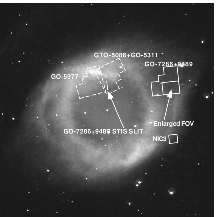
Figure 1.— This image of the Helix Nebula in H$\beta$ (O1998) shows the location of the apertures of the several data sets used in this study and HST program number that lead to their creation. This figure is similar to Figure 7 in O2002, except that the correct position angle of the STIS slit (PA=6°) is shown and the WFPC2 and NIC3 coordinated parallel fields are shifted accordingly. The image is 1180″x 1180″ and north is up.

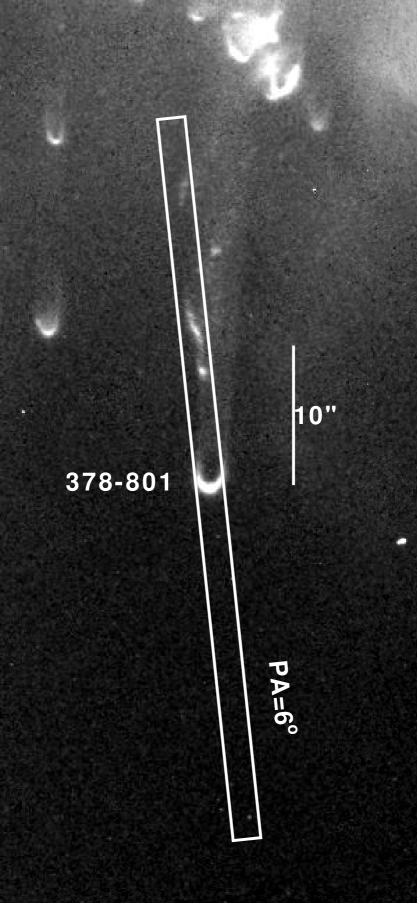
Figure 2.— This is a 30″x65″ section of the sum of the GTO-5086 and GO-5311 flux calibrated observations of H$\alpha$ and [N II], with the knot 378-801 near the center. The rectangle indicates the boundary and of the 2″x52″ slit used for the STIS observations discussed in this paper. North is up. The features about 10″ north of the bright cusp of 378-801 may be structure in the tail of this knot or may be a second knot that falls within the radiation shadow of 378-801.

This knot was observed with the Space Telescope Imaging Spectrometer (STIS, Woodgate et al. 1998) through its 2″x 52″entrance slit. Since the bright cusp of this knot is smaller than the width of the entrance slit and the radiation is dominated by emission lines, STIS was able to form monochromatic images in the various lines, essentially functioning as a slitless spectrograph. This pointing was the same as that employed in program GO-7286. The location of the entrance slit as projected on the nebula is shown in Figure 1 and Figure 2. Because of the paucity of candidate guidestars, the slit was oriented with PA=6°, as were the observations in program GO-7286.

Observations were made with multiple tilts of gratings G430M and G750M. A central wavelength setting of 4961 Å (2340 seconds exposure) gave useful observations of the H$\beta$4861 Å, and [O III] doublet 4959 Å and 5007 Å lines. A central wavelength setting of 6252 Å (4620 seconds exposure) gave useful observations of the [O I] doublet 6300 Å and 6363 Å. A central wavelength setting of 6581 Å (4620 seconds) gave useful observations of the same [O I] lines, the H$\alpha$ line at 6563 Å and the adjacent [N II] doublet 6548 Å and 6583 Å. These images were pipe-line processed by the STScI and flux calibrated using their system that is tied to observations of standard stars through the same instrument configuration. The resulting images have pixel sizes of 0.05″.

2.2. Imaging Observations

The wide field of good focus and large data storage capability of the HST allows the making of parallel observations. WFPC2 (Holtzman et al. 1995) and NICMOS (Thompson et al. 1998) observations were made during all of the primary target STIS observations. Since the primary target determines the pointing of the spacecraft, one gets what is available in terms of the parallel observations. However, the STIS slit could be placed in two orientations of 180° difference. We chose an orientation of the slit so that both the WFPC2 and NICMOS fields would fall onto the main body of the nebula.

The WFPC2 parallel field falls in a region outside of the main bright ring of emission of the Helix and in the zone that may be the projection of the more distant rotational axis of the nebula, which is a thick disk accompanied by perpendicular low density plumes (O1998, M1998).

2.2.1 WFPC2 Observations

We made WFPC2 images of the field shown in Figure 1 in four filters. There were six exposures in F656N for a total exposure time of 5600 seconds, six exposures in F658N (6600 seconds total), four exposures in F502N (4000 seconds total), and three exposures in F547M (300 seconds total). The multiple exposures were made to allow us to eliminate random events caused by cosmic rays. The F502N filter primarily isolates [O III] 5007 Å emission, while F656N is dominated by H$\alpha$ 6563 Å emission, and F658N is dominated by [N II] 6583 Å emission. However, each filter is affected by the underlying continuum and the F656N and F658N filters are both affected by H$\alpha$ and [N II] emission, the latter becoming important in the innermost knots which have much stronger [N II] emission than H$\alpha$ emission. These observations were pipe-line processed at the STScI, then combined with a similar set of observations made during program GO-7286, where the pointing was almost identical and the total exposure times were: F502N (4200 seconds), F547M (300 seconds), F656N (4600 seconds), F658N (2200 seconds). These images were then rendered into monochromatic, calibrated emission line images using the technique of O’Dell & Doi (1998), which corrects each filter for (any) contaminating non-primary line and the continuum and gives an image whose intensity units are photons cm^-2 s^-1 steradian ^-1.

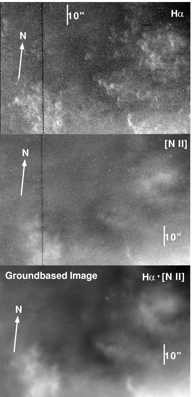
Figure 3.— The top two images show a portion of the combined images in H$\alpha$ and [N II] created in programs GO-7286 and GO-9489. The field of view of each is 95″x66″ and the vertical axis is pointed towards PA = 6°. Contrary to most images of photoionized nebulae, the knots are much sharper in H$\alpha$. The vertical dark line is caused by the seam between WFPC2’s CCD2 and CCD3. The lowest image is the same field in an unpublished H$\alpha$+[N II] image made by O’Dell with the MOSAIC camera on the CTIO 4-meter telescope under seeing conditions of fwhm = 0.9″.

The H$\alpha$ and [N II] images are shown in Figure 3. There are many indications of knots of emission, although only a few well defined bright cusps are seen. The features are much sharper in H$\alpha$ than in [N II], an unusual trend which is consistent with the result found in an earlier study using both slitless spectroscopy and imaging (OHB2000). The lowest portion of Figure 3 gives a comparison of the HST WFPC2 images with a groundbased H$\alpha$+[N II] image made with the MOSAIC camera of the 4-m Blanco Telescope of the Cerro Tololo Interamerican Observatory (CTIO). This image was made during a period of astronomical seeing with a measured fwhm = 0.9″ and a pixel size of 0.27″. We see that the bright regions of about 15″ diameter are broken up into multiple and often overlapping bright cusps with chord sizes about 2″. The image shows only diffuse faint emission in [O III], which is not surprising since it lies outside of the primary zone of [O III] by the nebula and the knots are known to emit little energy in this ion (M1992, OH1996, OHB2000).

2.2.2 NICMOS Observations

We also made parallel observations with all three cameras of the NICMOS instrument. Because of the filter combinations available and the lack of simultaneous focus, in part due to an error in the observing program, only the NIC3 detector results were useful for this study and even its images are out of focus. That camera has an array of 256x256 pixels, each subtending 0.2″x0.2″. We made four exposures (total exposure times of 10,752 seconds in each) in both the F212N filter and the F215N filter. The F212N filter primarily isolates the H₂ 2.12 µm line and the F215N filter the adjacent continuum. The field imaged is shown in Figure 1 and is almost identical with the field observed in program GO-7286. These new images were not averaged with the older data because there is always a certain amount of degradation of resolution in combining two not-identical-pointing images, the new images are better spatial resolution, and the earlier observations were of only 3326 seconds (F212N) and 3582 seconds (F215N).

The NIC3 images are significantly out-of-focus, but some information can be obtained from them. The stars in our field of view have central dips of about 30% and a full width half maximum (fwhm) value of 9 pixels. This means that we cannot hope to resolve nebular H₂ structures of less than 1.8″.

The images were subjected to the STScI’s pipe-line data processing, which gave corrected count-rates (CR) per pixel in each detector. The instrument data handbook (section 5.3.4) gives for the calibrated flux (Flux, in ergs s^-1 cm^-2) from an emission line Flux=1.054xFWHMxPHOTFLAMxCR, where FWHM is the full width at half maximum of the filter and PHOTFLAM is a sensitivity constant determined from observations of a calibrated continuum source. In using this equation the assumption has been made that the emission line is at the center of the filter (a good assumption for this low velocity source) and that the continuum contribution has been subtracted (discussed in this section). Inserting the tabulated values of FWHM = 202 Å and PHOTFLAM = 2.982 x 10^-18 gives Flux = 6.35 x 10^-16. We corrected for the continuum by examination of a section of the image that contained no evidence of knots, normalizing F215N filter signal to be the same as the F212N image in that section, then subtracting the normalized F215N image from the F212N image. After scaling into surface brightness (S_2.12μ in ergs s^-1 cm^-2 sr^-1) and trimming a bad edge, one has the image shown in Figure 4, where the average value of S_2.12μ is 1.0 x 10^-5 ergs s^-1 cm^-2 sr^-1 and the peak value is 5 x 10^-5 ergs s^-1 cm^-2 sr^-1. The intrinsic values of S_2.12μ will be higher by an amount determined by the defocus. However, we should be able to determine accurate total fluxes for the individual knots. These points are addressed in § 4.3, where we also compare our values with groundbased observations.

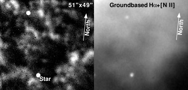
Figure 4.— The left image is the out-of-focus 51″x 49″ NIC3 parallel image in continuum subtracted values of S_2.12μ. The image has been rotated so that the vertical axis is at PA=6° in order to nearly match the orientation shown in Figure 1. The average value of S_2.12μ is 1.0 x 10^-5 and the peak value is 4 x 10^-5. Correction of the peak values of S_2.12μ for the instrumental fwhm being greater than the cusp shaped area of the emitting regions is discussed in the text. The characteristic fwhm of the stars is about 1.8″. The right image is the matching field from the same H$\alpha$+[N II] image used in Figure 3.

3. ANALYSIS

3.1. Analysis of the WFPC2 Images

Studies of the variation in the peak surface brightness of the cusps with angular distance from the central star have been made previously (OH1996, López-Martín et al. 2001) within the expectation that this would be a useful diagnostic of the knots. This is because each cusp represents a local ionization front and to first order their surface brightness in a recombination line such as H$\alpha$ should scale linearly with the incident flux of LyC photons so long as the cusps are in static ionization equilibrium, with recombinations balancing photoionizations. OH1996 demonstrated that the cusps were significantly fainter than expected from this simple argument and López-Martín et al. (2001) found from the careful study of a few knots that this deficit of emission could be explained by advection of neutral hydrogen from the core into the cusp, which represents an additional sink of ionizing photons and leads to a reduced rate of recombinations compared to the static case.

In the light of the fact that we now have calibrated H$\alpha$ and [N II] data that cover a much wider range of angular distances from the central star than in other studies, we have re-executed an analysis of the brightness of the cusps.

We have measured the peak cusp surface brightness for 530 knots identified in the WFPC2 fields of programs GTO-5086, GO-5311, and GO-5977 (OH1996, OB1997) and an additional 70 in the WFPC2 field obtained in this study (§ 2.2.1). The brightness of each cusp was measured in a 2x5 pixel box centered on the brightest portion and oriented with the long axis perpendicular to a line towards the central star. The nebular surface brightness used for correction of the cusp signal was determined from a nearby 5x10 pixel box. A similar analysis of the [N II] image was done for each object, but the cusp sample box was shifted 0.8 pixels towards the central star. The knot cores were also sampled in [O III] using 5x5 pixel boxes that were shifted 7 pixels away from the central star with respect to the H$\alpha$ cusp.

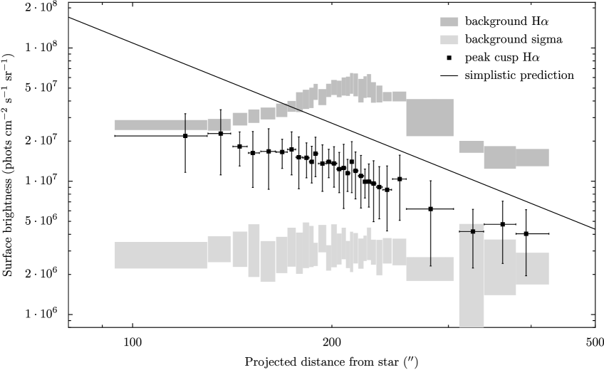
Figure 5.— The peak H$\alpha$ surface brightness of the knot cusps (filled circles), the nebular brightness (dark grey boxes), and the standard deviation of the nebular brightness (light grey boxes) are shown as a function of the distance from the central star. The boundaries of the boxes indicate the one sigma boundaries about the mean values. The solid line is the predicted relation under the assumptions of the knots being viewed face-on, the distance from the central star being that indicated by the angular separation, and diminution of LyC radiation by advected neutral hydrogen being unimportant. In the case of failure of each of these assumptions, the expected surface brightness would be lower than this prediction.

The results for H$\alpha$ of this analysis are shown in Figure 5. In this figure we show the surface brightness for H$\alpha$ and the standard deviation of the nearby nebular emission for a box of the same size as used for extracting the cusp brightness. The results indicate that we have traced the cusps out to where they are lost in the fluctuations of the nebular background. The upper line is the expected relation if all of the knots were viewed face-on and were located at the distance indicated by their angular separation (these are mutually exclusive conditions). This is the same method of calculation as OH1996, except the more recent value of the total flux of the nebula of F(H$\beta$)=3.37x10^-10 ergs cm^-2 s^-1 (O1998) was used. This method of calculation also ignores the effects of advection. In practice, few of the knots will be viewed in the plane of the sky. Most will be at foreground or background positions that will place them further from the central star than indicated by their angular separations, and some advection will be present. Each of these factors will cause the expected surface brightness to be less than the line labeled “simplistic predictions”. Limb brightening would tend to work in the opposite direction by raising the cusp brightness, but this is evidently less important than the first two effects.

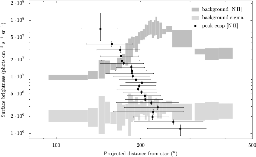
Figure 6.— This figure is similar to Figure 5, except that it presents the results of the analysis of [N II]. In addition to the [N II] for the cusps (filled squares), we also give the values for nearby portions of the nebula (filled boxes). The cusp [N II] emission becomes weaker at greater distances and the nebular emission shows a relative increase. Negative values indicates that the [N II] appears fainter than the nebular surroundings.

The characteristics of the nebula and the knots in [N II] are summarized in Figure 6., where we see that the cusp brightnesses monotonically decrease with increasing distance from the central star, while the nebular brightness peaks at about 210″. The nebula’s peak is due to reaching the ionization front that confines the inner-disk and outer-ring, these being seen at about the same distance from the central star in the northern sector (OMM2004), which numerically dominates this sample.

It is difficult to determine a trend of [O III] emission from in front of the bright cusps, but, there is a weak correlation of increasing emission with decreasing projected distance from the central star.

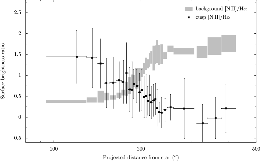
Figure 7.— This figure gives the [N II]/H$\alpha$ ratio at the position of the knots.

The ratio of [N II] lines and the H$\alpha$ line cusp emission is shown in Figure 7. We see that [N II] becomes fainter relative to H$\alpha$ with increasing distance, whereas in the nebula the opposite is true. Each cusp is a microcosm of the nebula as a whole and should show all the ionization stages up to the highest stage seen in the local surrounding nebula. However, although the large-scale nebula is probably very close to photoionization equlibrium, the cusps themselves most certainly are not if they do indeed represent photoevaporation flows. This is because the dynamical time for the gas to flow away from the cusps is the same order as the photoionization timescale.

For gas in static photoionization equilibrium the ionization state at a given point is governed by the balance between recombinations and photoionizations, according to the local electron density and radiation field, with the latter being strongly affected by the photoelectric absorption of H and He. For example, at larger radii in our observations the line of sight progressively becomes dominated by the helium neutral zone (from which [N II] emission primarily arises) as the ionization front of the inner-disk and the outer-ring is approached.

On the other hand, for very strongly advective flows, such as are found in the knot cusps, recombinations are unimportant and the ionization state at a given point is given merely by the photoionization rate (cross section times ionizing flux) and the length of time since the gas was first exposed to ionizing radiation. Furthermore, the effective extreme ultraviolet optical depth to the ionization front is low (of order unity) so that radiative transfer effects are relatively unimportant, except for at low ionization fractions. The simplicity thus gained, however, is offset by the complication that the ionization state is now intricately linked to the gas dynamics. One will still find an ionization stratification but, since the cause is now different, one may see a difference in the detailed distribution of the ions.

The thermal balance in the ionized gas is also affected by the advection since “adiabatic” cooling due to the gas acceleration and expansion can become comparable to the atomic cooling. The relative importance of advection in the cusps is expected to increase as the ionizing flux decreases so knots that are farther away from the star might show lower temperatures in their photoevaporation flows. This is one possible explanation for the reduction in the [N II]/H$\alpha$ ratio with distance, which is explored more fully in § 4.2 below.

Knots in PN are almost unique in their exemplification of this extreme regime of photoevaporation flows (Henney 2001). HII regions are generally in the opposite “recombination-dominated” regime where the effects of advection are considerably subtler (Henney et al. 2005b). The Helix knots are therefore an important laboratory for testing our understanding of the physics of this regime.

3.2. Analysis of the STIS Slitless Spectrum Images

As described in § 2.1, the slitless images were made at three grating settings. In several cases these included line doublets ([O I] 6300+6364 Å, [N II] 6583+6548 Å, and [O III] 5007+4959 Å). Since each of these doublets arise from the same upper levels, the ratio of intensity of the components is constant and in each case is close to three to one. This means that we were able to derive higher quality images characteristic of each ion by combining the separate images of lines, a possibility exploited further through the fact that the [O I] lines appear at two grating settings, with the result that images of four lines are available. The H$\alpha$ + [N II] image is similar to that shown in Figure 1 of OHB2000 in that the shorter wavelength [N II] line image slightly overlaps H$\alpha$. We circumvented this problem by scaling, shifting and subtracting the image of the clearly separated longer [N II] line. The results are shown in our Figure 8. We see that the [N II] emission is predominantly outside of the reference circle centered on the knot, whereas the [O I] emission peaks at roughly the same position as H$\alpha$. The radii and FWHM of the peak of the cusp emission are: [O I] 0.52″ and 0.21″, [N II] 0.58″ and 0.30″, H$\alpha$ 0.54″ and 0.20″.

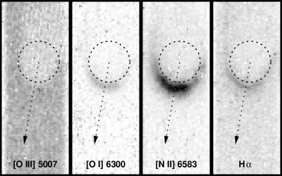
Figure 8.— Each of these panels shows the composite image for the various key ions in our analysis. They were formed from adding the appropriately scaled images of forbidden line doublets and the H$\alpha$ image was corrected for the slightly overlapping [N II] 6548 Å line’s image. The circle identifies the knot core and is in the same location in each panel. The arrow indicates the direction towards the central star.

Figure 9.— Radial profiles of emission line surface brightness images of knot 378-801 as measured from the nominal knot center. Symbols show all pixels whose radius from the knot center makes an angle $\theta$ of less than 30° with respect to the direction to the central star. A heavy solid line shows a smoothed version of the same data, while the lighter lines show 15° subranges in $\theta$ between 0° and 90°.

A more thorough presentation of the characteristics of the cusp are shown in Figure 9. In this figure we show the profiles of each of the ions, now including [O III], for all of the data within 30° from the direction to the central star. The different cusp widths and location of their peaks is well illustrated. It is obvious that the progression is not that expected from a simple ionization front, where the [O I] emission would be much narrower and clearly displaced towards the knot center, the [N II] emission would be further out and only slightly wider, and the H$\alpha$ emission would be broadest and peak furthest from the knot center.

The explanation for this anomalous progression probably lies in the strong departures from static photoionization and thermal equilibrium in the cusps, as discussed in § 3.1. OHB2000 could successfully reproduce the distribution seen in earlier observations by assuming a gradual rise in temperature of the gas as it becomes ionized. This is in contradiction to the usual structure of an ionization front, in which the gas temperature rises to close to its equilibrium ionized value ($\sim 10^{4}$ K) before the gas becomes significantly ionized (Henney et al. 2005b). The OHB2000 model is unsatisfactory in that the temperature structure was imposed in a totally ad hoc manner. This is rectified in § 4.2 below, where we present self-consistent radiation hydrodynamic models of the flows from the cusps.

3.3. Analysis of NIC3 H₂ Images

The best resolution groundbased study of H₂ in the entire Helix Nebula is that of S2002, who imaged the entire nebula. Although their angular resolution is not stated, the pixel size employed was 2″ and the astronomical seeing was probably no worse than that, which means their effective resolution it is comparable to the degraded focus fwhm of this study. Their image shows a few bright features within our NIC3 field, but our images go fainter than their limit and show many more knotty structures. Except for the east-west feature in the upper central portion of our Figure 4, there are no other features that correlate with the groundbased image.

In our images there is no indication of the cusp structure seen in the optical emission lines, which all arise from photoionized gas, but there are numerous emitting knots with a characteristic fwhm of 2.3″. In no cases do we see the central dips characteristic of the defocused star images, which means that the intrinsic size of the H₂ cores are larger than a few pixels (about 0.5″). A Gaussian subtraction of the stellar fwhm (1.8″) from the average knot fwhm (2.3″) indicates an H₂ emitting core of fwhm = 1.4″, which is comparable to the size of the cores of the knots as outlined by extinction in [O III]. We do not see an elongation of the knots along a direction perpendicular to a line directed towards the central star which is what we would expect if this emission came from a cusp-shaped form. However, the theoretical expectation is that the H₂ emission should come from a cusp shaped H₂ zone lying between the emission line cusp and the central core of the knot. These cusps would have to have elongations almost equal to the instrumental fwhm in order for us to have seen them. When we do see evidence of cusp structures, they are always large, knotty, and have random orientations, indicating that they are chance superpositions of individual H₂ emitting knots.

An examination of F212N images of a southeast outer ring section of the Helix Nebula made as part of program GO-9700 is useful. These images are in good focus, with stellar images of fwhm=0.3″; however, the exposures showing knots were only 384 seconds duration and a thorough discussion of those images will not be made here. The H₂ emission appears as cusps of the same form as those seen in ionization in the inner nebula. These cusps are about 0.4″ thick and 1.8″ wide. As noted in the previous paragraph, this type of image would not produce any noticeable elongation of our reduced resolution images.

The images show that the brightest knots in our NIC3 field have values 4 x 10^-5 ergs s^-1 cm^-2 sr^-1, which is much less than the values for the same region of greater than 10^-4 ergs s^-1 cm^-2 sr^-1 indicated in Figure 6 of S2002. The instrumental broadening of both sets of data could mean that the instrinsic surface brightness of the knots is higher than we give, but the comparable spatial resolution of both means that this cannot be the explanation of the differences between them. S2002 does not report that any correction was made for continuum radiation in their H₂ filter, which could indicate that the overestimate could be due to underlying continuum. In our filter system the signal from the F212N filter was about 80 % due to continuum, as determined from the F215N filter. S2002 did not detect the Br $\gamma$ line at 2.166 µm, with an upper limit of 7 x 10^-8 ergs s^-1 cm^-2 sr^-1, which means that it is not a source of contamination of the F215N filter that we have used as a continuum reference.

We can approximately correct our peak surface brightness values using the information from the GO-9700 images. If the cusps have a rectangular size of 0.4″x 1.8″ and our circular images have a diameter of 2.3″, then the scaling factor from our observed peak surface brightness to the intrinsic peak surface brightness will be $\pi$1.15²/0.4x1.8=5.8. This means that the observed peak surface brightness in our images (4 x 10^-5 ergs s^-1 cm^-2 sr^-1) would have intrinsic (corrected) values of 2.3 x 10^-4 ergs s^-1 cm^-2 sr^-1.

A comparison of the HST NIC3 H₂ image with the CTIO groundbased H$\alpha$+[N II] image is made in Figure 4. In this figure we see that there is no obvious correlation of the ionized gas emission with the H₂ emission. This far out from the central star the radiation is dominated by low ionization emission (O1998, Henry et al. 1999), which would be [N II] in this case, and the surface brightness of the ionized cusps will have dropped to well below what can be resolved against the nebular background (for reference, see the discussion in § 4.1).

4. Discussion

In this section we present and discuss the interpretation of our observations. In order to make the best use of them, we have developed extensive theoretical models, the first combining radiation and hydrodynamic effects, in support of explaining the optical emission line observations, and the second is a static model of the molecular region, in support of explaining the H₂ observations. We combine our new observations, our new models, and existing infra-red and radio observations to develop a comprehensive model of the knots in the Helix Nebula.

4.1. A General Model for 378-801

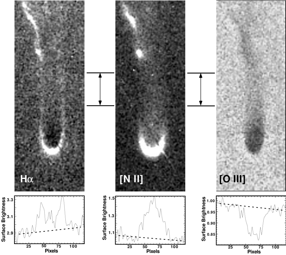
Figure 10.— The upper three panels show 5.9″x 16.2″ samples around 378-801 from the WFPC2 programs GTO-5086 and GO-5311 selected to lie along the symmetry axis of the tail, which coincides with a radial line drawn towards the central star. The pixel scale has been adjusted to 0.05″ in order to agree with that of the STIS images. The diagonal feature across the [N II] cusp is an artifact in the original image. The upper left feature in the H$\alpha$ and [N II] images is probably a partially shadowed second knot that is unrelated to 378-801. The bands between the upper panels show the range of rows that were averaged when making the tail profiles shown in the lower three panels. The limb brightening seen in H$\alpha$ contrasts with the concentrated emission seen in [N II] and the concentrated extinction seen in [O III].

We probably know more about the object 378-801 than any other knot in the Helix Nebula because of the wide variety of observations that have been made of it. The best optical image is that of OH1996, where the knot is the central object in their Figure 3. That source was used for preparing the monochromatic images shown in our Figure 10. The bright cusp is well defined in H$\alpha$ and [N II] with a central extinction core visible in [O III] emission. The tail is well defined, with nearly parallel borders. At 8.5″ away from the bright cusp there is a secondary feature that that starts on the east side of the tail and extends away from the central star without the bright cusp-form characteristic of other knots found this close to the central star. Its shape indicates that this is not a feature of the tail of 378-801, rather, that it is a second knot that lies nearly along the same radial line from the central star.

4.1.1 The Core

A molecular core in the knots was predicted by Dyson et al. (1989) before observational measurement and since then has been detected with increasing spatial resolution. 378-801 has been imaged in the CO J=1–0 2.6 mm line by H2002 with an elliptical Gaussian beam of 7.9″x 3.8″ having an orientation of the long axis of PA = 14°, that is, at 18° from the orientation axis of the object. In that image one sees two peaks of CO emission, one on-axis 3″ from the bright cusp and a second associated with the overlapping feature, with a peak at 8″ from the bright cusp. Since they used the lower spatial resolution groundbased images of (M2002) for reference, they interpret this feature as part of 358-801’s tail, which it clearly is not. They also observed the object in the H₂ 2.12 µm line under conditions of seeing of 1.2″ and found a slightly broadened source just inside the curved optical bright cusp, having a surface brightness of about 10^-4 ergs s^-1 cm^-2 sr^-1 (using the S2002 images for calibration). This image is consistent with the small cusps one sees in the southwest region of the Helix imaged in H₂ as part of program GO-9700 (§ 3.3). The CO source in the tail of 378-801 has a peak emission at V${}_{\hbox{$\odot$}}$=31 km s^-1 (H2002 give V${}_{\hbox{$\odot$}}$=V_LSR - 2.9 km s^-1 and they work in LSR velocities). This velocity agrees well with V${}_{\hbox{$\odot$}}$= 31.6 $\pm$1 km s^-1 derived from optical spectra by M1998, which means that there is not a large relative velocity of the CO source within the tail and its associated knot.

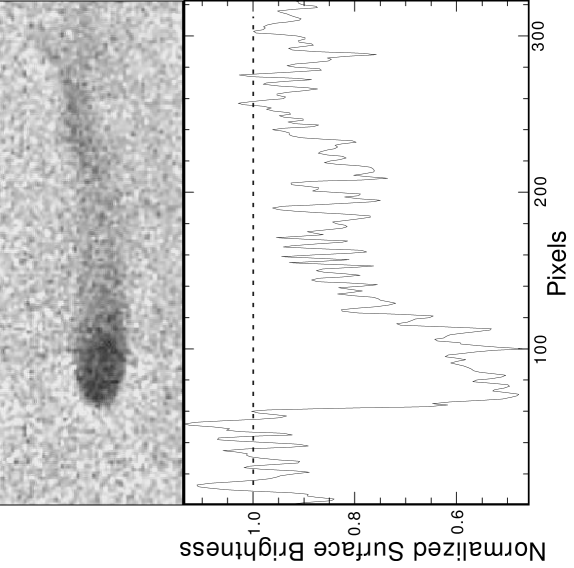
Figure 11.— The top panel in this figure is the same as the [O III] image in Figure 10. The lower panel shows a trace 0.15″ wide along the symmetry axis of the cusp and tail. This illustrates not only the concentration of extinction to the core of the knot, but that there is material that extends out to where the the adjacent source confuses matters at about pixel number 200.

The distribution of dust within 378-801 is best determined by tracking the extinction of background nebular emission in the light of [O III], since the knot has little intrinsic [O III] emission. Figure 11 shows a trace of the surface brightness along the symmetry axis of the knot and its tail, after normalizing the local background to unity. The maximum extinction gives a contrast of 0.5, which corresponds to an optical depth of 0.69. This value will be a lower limit if the knot does not lie in front of all the nebular [O III] emission. That seems to be the case, as M1998 give high resolution spectroscopic evidence (their § 5.1) that the knot is causing extinction only in the redshifted component of the nebula’s light. This value of the optical depth is probably underestimated since the nebular light will slightly fill-in the central region due to the finite point spread function of the WFPC2 (McCaughrean & O’Dell 1996). Using the method of determination adopted by OH1996 (which is similar to that of M1992) and a gas to dust mass ratio of 150 (Sodroski et al. 1994), gives for a lower limit to the mass within the entire core (a sample of 2.1″x 2.3″ centered on the core) of 3.8x10^-5 M_sun. This is similar to the lower limit of 1x10^-5 M_sun found from the CO observations for 378-801 and its nearby trailing feature (H2002). The peak extinction corresponds to a lower limit of the column density of hydrogen of 1.7x10²¹ hydrogen atoms cm^-2. If this material is concentrated to a distance corresponding to 1″  then the central hydrogen density of the knot is at least 5.2x10⁵ cm^-3.

As shown in § 3.2, the appearance of H₂ emission in a cusp just behind the ionized cusp is what is expected for a progression of conditions going from the outer ionized gas, through atomic neutral hydrogen, then H₂. The innermost region of the core would be coldest and have the most complex molecules.

4.1.2 The Tail

The appearance of the tail will be a combination of the properties of the gas and dust found there and the photoionization conditions. A longitudinal scan of the cusp and tail in [O III] was shown in Figure 11 and a cross sectional profile of a section of the tail was shown for H$\alpha$, [N II], and [O III] in Figure 10. Taking the [O III] extinction as a measure of the total column density and assuming axial symmetry, it appears that the tail is a centrally compressed column of material that decreases slowly in density with increasing distance from the center of the knot. The cause of this distribution is unknown, although it is consistent with the acceleration of the neutral gas via the rocket effect, e.g. (Mellema et al. 1998). The low relative velocity of the core and the CO peak in the tail (§ 5.1.1) argues that this reflects the initial distribution of material following the formation of the core through an instability followed by radiation sculpting of the tail (O2002)

Within the LyC shadow of the core the conditions will be very different from those in the nebula. This condition has been theoretically modeled by Cantó et al. (1998) and those models have been compared with observations of the knots in the Helix Nebula and the the proplyds in the Orion Nebula (O’Dell 2000). Material in the shadow will only be illuminated by diffuse photons of recombining hydrogen and helium, with the most important being hydrogen. Because most of these recombinations will produce photons only slightly more energetic than the ionization threshold of hydrogen, whereas the stellar continuum is emitted mostly at higher energies, the average energy per photon given to the gas in the shadow will be much lower than in the nebula and the electron temperature will be about two-thirds that of the nebula (Cantó et al. 1998, Osterbrock 1989). If the gas density within the shadow is sufficiently high, then there will be an ionization progression much like when one approaches the ionization front of an H II region, with a neutral core in the middle. If the gas density is low, then complete ionization of the shadow region will occur.

Our profiles in H$\alpha$ and [N II] across the tail shown in Figure 10 are very different. In H$\alpha$ we see strong limb-brightening, as if we are seeing a cylinder of emission edge-on. In [N II] we see that the emission is very similar to that of the total column density of material, as measured by the [O III] extinction. The well defined H$\alpha$ boundary makes it appear that only the outer part of the tail is photoionized. However, to create the collisionally excited [N II] lines, one needs both electrons of several electron-volt energy and singly ionized nitrogen. It is obvious that a more sophisticated photoionization model is required and the paper by Wood, et al. (2004) is a step in this direction, although it is not directly applicable to this knot because they only consider a shadow formed in a region surrounded by only singly ionized helium.

4.2. Models of the Knots that combine Hydrodynamics and Radiation

In order to model the properties of the ionized flows from the cometary knots, we have carried out a preliminary numerical study of the dynamical evolution of a dense neutral condensation, subject to the effects of stellar ionizing radiation. The simulations were carried out by means of the radiation-hydrodynamics code described in Henney et al. (2005a). The initial conditions for the simulation were a cylindrical concentration of dense neutral gas, with core radius $2\times 10^{15}$ cm and density $3\times 10^{4}$ cm^-3, which was illuminated by the ionizing spectrum similar to that of the Helix central star ($T_{\mathrm{eff}}=120,000$ K; ionizing luminosity $Q_{\mathrm{H}}=7.8\times 10^{45}$ s^-1). The local diffuse field is treated in the on-the-spot approximation and the global nebular diffuse field, with an expected strength of only 1–4% of the direct radiation (Lopez-Martín et al. 2001), is neglected. The only source of opacity considered in the simulations is photoelectric absorption (the dust optical depth through the ionized flow ion the ionizing ultraviolet is only of order 0.01 and can be safely neglected). Free-expansion conditions were used on the grid boundaries, which is reasonable since the ionized flow becomes supersonic. A simple ram-pressure balance argument indicates that the stand-off shock between the ionized globule flow and the ambient nebular gas should occur at about 50 times the globule radius, which is outside our computational grid. Any wind that may exist from the central star is confined very close to the center of the nebula (Zhang, Leahy, & Kwok 1993) and does not affect the knots.

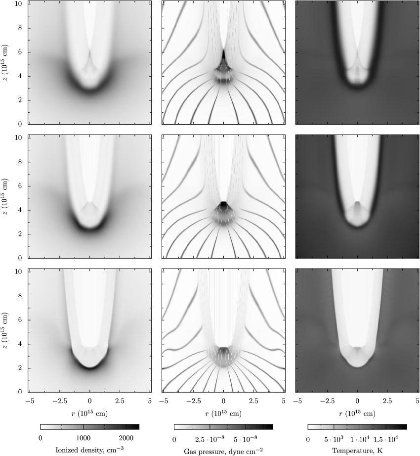
Figure 12.— Physical structure of the model simulations at an age of 132 years for a knot at a distance of $4.63\times 10^{17}$ cm from the ionizing star. The three rows of panels show simulations calculated using different degrees of hardening for the ionizing radiation (most hardening in the top row, no hardening in the bottom row). The three columns show, ionized gas density, gas pressure, and gas temperature, from left to right. The central column also shows contours of the initial cylindrical radius of the gas at each point, which serve as approximate streamlines for the ionized part of the flow.

Models were run with the globule located at various distances from the star between $3\times 10^{17}$ and $10^{18}$ cm, and the evolution was followed for approximately 500 years. A snapshot of the structure of a typical model is shown in Figure 12.

The photoevaporation of the surface layers drives a shockwave through the knot, which compresses it and accelerates it away from the ionizing star (Bertoldi 1989, Mellema et al. 1998, Lim & Mellema 2003). In our simulations, the neutral clump reaches speeds of order 2 to 5 km s^-1. At the same time, an ionized photoevaporation flow develops from the head of the clump, which accelerates back towards the star, eventually reaching speeds of order 20 km s^-1. The bulk of the optical line emission is produced by denser, slower-moving gas from the base of the photoevaporation flow, near the ionization front, as can be seen in the left-hand panels of Figure 12, which show the ionized gas density. Three models are shown, which differ in their treatment of the hardening of the radiation field, which is treated only very approximately in the current simulations. In the model with maximum hardening (upper panels), the ionization front is very broad and the gas temperature (right panels) has a pronounced maximum on the neutral side of the front. When the hardening is reduced (lower panels), the front is much sharper, with a less pronounced temperature peak. The pressure of the photoionized flow (central column of panels) is also higher in the models with greater hardening and, as a result, a stronger shock is driven into the neutral knot. Weaker shocks are also driven in from the flow from the sides of the knot, which eventually converge and bounce off the symmetry axis, as in the upper model of Figure 12.

Although these two-dimensional simulations do not contain all the details of atomic physics that have been included in one-dimensional models (e.g., Henney et al. 2005b), they nonetheless capture the most important physics of the photoionized flow, which is dominated by photoelectric heating and expansion cooling, and therefore they can provide a tool for investigating the physical basis of the observed optical emission properties of the knots. The most important of these are that the [N II]/H$\alpha$ ratio falls precipitously with distance of the knot from the central star (§ 3.1) and that the [N II] emission from the best-studied individual cusps is found to lie slightly outside the H$\alpha$ emission (§ 3.2). OHB2000 attempted to explain the second of these by positing an ad hoc broad temperature gradient in the photoevaporation flow, leading to enhanced collisional line emissivity and depressed recombination line emissivity at greater distances from the knot center.

We have calculated for each model the emission properties of the cusps as follows. First, we automatically identified the ridge in the ionized density at the cusp and fit for its curvature. Using the position and curvature of the cusp we determined a nominal center for the knot. Then, we derived radial emissivity profiles as a function of distance from the knot center, averaging over all radii within 60° of the symmetry axis. From these profiles, we calculated the mean surface brightness of the cusp and its mean radius from the knot center for each emission line. These steps were carried out for each of a sequence of times in the evolution of the knot up to an age of $\simeq 500$ years, which were finally averaged to give a global mean and standard deviation for each model. In the final averaging the initial 50 years of evolution were omitted since this represents a highly non-steady phase in which the flow is still adjusting to its quasi-stationary configuration.

The lines that we considered were H$\alpha$ and [N II] 6583 Å, with temperature-dependent emission coefficients that were calibrated using the Cloudy plasma code Ferland (2000). The ionization fraction of nitrogen was assumed to exactly follow that of hydrogen and double-ionization of nitrogen was neglected (the extreme weakness or absence of [O III] emission from the cusps indicates that this is a reasonable approxmation).

Figure 13.— Model predictions for knot cusp radius as a function of distance from the central star. Lower panel: mean radius of H$\alpha$ emission from cusp in arcseconds. Upper panel: ratio of mean cusp radius in [N II] to that in H$\alpha$. Vertical bars indicate the range of values during the evolution of the models. Different symbol types correspond to models with differing treatment of the radiation hardening and photoelectric heating (see text).

Figure 14.— Model predictions for knot surface brightness as a function of distance from the central star. Lower panel: face-on surface brightness of H$\alpha$ emission from cusp. The dotted line shows the simplistic prediction as in Figure 5. Upper panel: ratio of [N II] surface brightness to that of H$\alpha$. Symbol types are as in Figure 13.

The results are shown in Figures 13 and 14 and for two different sets of models, which differ in their treatment of the hardening of the radiation field and in the contribution of helium to the photoelectric heating. The upper panel of Figure 13 shows that the mean radius of the [N II] emission is indeed larger than that of H$\alpha$, but only significantly so for knots that are farther than 200″ from the central star. This is a direct result of the temperature structure in the ionized flow, which has a maximum close to the peak in the ionized density. For the farther knots, this temperature peak is slightly outside the ionized density peak, which biases the [N II] emissivity to larger radii.

The upper panel of Figure 14 shows that the [N II]/H$\alpha$ surface brightness ratio of the knots does decline with distance, particularly for the model with less hardening. This is a direct result of the flow not attaining such high temperatures when the knot is further from the star, which is due to the increased relative importance of “adiabatic” cooling as the flow accelerates. However, although this behavior is in qualitative agreement with the observations, the decrease seen in the models is much less sharp than is seen in the real nebula. It should also be noted that we have had to assume a nitrogen abundance of $\mathrm{N/H}=1.2\times 10^{-4}$ in order for the absolute values of our [N II]/H$\alpha$ ratio to be consistent with the observations. This is roughly two times lower than the abundance that has previously been derived for the nebula as a whole (Henry, et al. 1999).

The N abundance that we find from our models is close to the solar value and is very similar for the models with different hardening. Although this could be interpreted as evidence for differing abundances between the knots and the rest of the ejecta, we do not think that such an inference is warranted. The photoionization models on which previous abundance studies have been based are only very crude representations of the 3D structure of the nebula, so that their derived abundances are probably not reliable.

The lower panel of Figure 14 shows the dependence on distance of the H$\alpha$ cusp surface brightness of the models. The values shown are for a face-on viewing angle and thus should by multiplied by a factor of a few to account for limb-brightening. Once this is taken into account, they are in very good agreement with the observed values (Figure 5), and in particular fall well below the line derived from equating recombinations in the flow to the incident ionizing flux, which is an illustration of the importance of the advection of neutrals through the front, as discussed in López-Martín et al. (2001).

It is heartening that our simple radiation-hydrodynamic models are qualitatively consistent with the trends seen in the observations, although there are some quantitative discrepancies. In particular, in the models, both the reduction in the knot [N II]/H$\alpha$ surface brightness ratio and the increase in the size of the [N II] cusp relative to the H$\alpha$ cusp only occur at large distances from the central star, whereas in the Helix they are observed to occur at smaller distances. Although this may be in part a projection effect, due to the projected distances of the knots being smaller than their true distances, that is unlikely to be the whole explanation. One possibility is that the farther knots see a much reduced ionizing flux due to recombinations in the nebula between them and the ionizing star, whereas in our models we assume only a geometric dilution of $1/r^{2}$.

It is also possible that some of the atomic physics processes that have been neglected in our models may prove important in determining the thermal structure. More realistic simulations are in preparation and it remains to be seen if they will lead to an improvement in the agreement with observations.

4.3. H₂ Emission

In addition to the surface brightness in the H₂ 2.121 $\mu$m line discussed in § 3.3, there is the important and constraining result of Cox et al. (1998), who determined from ISO spectrophotometry of six H₂ lines that this gas has an excitation temperature of 900 K. In this section we will show that radiation-only-heating models cannot explain such a high temperature.

The other basic constaint is the column density of H₂. If the molecular gas is in LTE then the surface brightness in an optically thin line is simply related to the gas column density. We adopt a 2.121 $\mu$m H₂ line surface brightness of 2.3x10^-4 ergs cm^-2 s^-1 sr^-1. At 900 K, we expect

$$S(\mathrm{H_{2};\ 2.121~{}\mu m})=3.83\times 10^{-24}N(\mathrm{H_{2}})~{}\mathrm{erg\ cm^{-2}\ s^{-1}\ sr^{-1}}$$

and obtain a column density of N(H₂)$\simeq$ 6x10¹⁹ cm^-2, or N(H)$\simeq$ 12x10¹⁹ cm^-2 if the gas is fully molecular. This warm H₂ layer has a physical thickness of 1.2x10¹⁵ cm (§ 3.2), so we find a density of $\rm n(\mathrm{H_{2}})=N(\mathrm{H_{2}})/\delta r\simeq 6\times 10^{4}~{}\mathrm{cm^{-3}}$. This is not significantly smaller than the density Cox et al. (1998) quote for H₂ to be in LTE. We assume this density in the remaining work.

Since the emissivity is driven by the excitation temperature, the cause of the high temperature must be resolved prior to comparing the observed and predicted surface brightness of the H₂ 2.121 $\mu$m line. We present our model in § 4.3.1, give an interpretation of the observations and derive the additional heating required in § 4.3.2, and other relevant observations of the core of the knots are discussed in § 4.3.3. A critique of previous comparisons of H₂ observations and models is presented in § 4.3.4.

4.3.1 The Predicted Knot H₂ Properties

For simplicity, we assume that the knot is illuminated by the full radiation field of the central star, a good assumption since the nebula is quite optically thin up to where knots are first detected. We assume a seperation from the central star of 0.137 pc, appropriate for the knot 378-801. We further assume that the knot has the same gas-phase abundances as the H II region (Henry et al. 1999). The illumination is assumed to be from a black body of 120,000 K and 120 $\rm L_{\odot}$ (Bohlin et al. 1982, adjusted to a distance of 213 pc). In addition, we assume an ISM dust-to-gas ratio and grain size distribution, but do not include PAH’s since Cox et al. (1999) report that no PAH emission is seen. We assume that the density is constant across the knot in our photodissociation calculations. Cox et al. (1999) convincingly argue that the lower levels of H₂ are in LTE and that this requires a density $n\geq 10^{5}$ cm^-3, which is much higher than the characteristic (1200 cm^-3) density in the ionized zone (OB1997).

Figure 15.— The gas temperature is shown as a function of molecular hydrogen column density for our Cloudy models of the knot PDR. The solid line shows a model calculated using our best estimates of parameters appropriate for the Helix knots. The dashed line is the t$=$4000 yr case considered by Natta & Hollenbach (1998). The largest difference is that the central star luminosity is about a factor of 40 larger. Grain photoelectric heating of neutral gas creates a significant warm (about 900 K) region.

With these assumptions the conditions within the knot can be calculated with no unconstrained free parameters. The solid line in Figure 15 shows the gas temperature as a function of the column density of molecular hydrogen as one goes into the knot. It can be seen that the column of warm H₂ is very low (about 10¹⁶ cm^-2 for T$>$900 K) and that the temperature has fallen to about 50 K before an appreciable column density is reached, much lower than the observed H₂ temperatures.

This result seems to conflict with NH1998, who found significant amounts of warm (900 K) molecular gas in their model for a PN envelope at an evolutionary age of 4000 years. We recomputed this case using the time-steady approximation and approximating the dynamics with constant gas pressure. While the time-steady assumption is not really appropriate for the H₂ transition region because of the long formation timescales, it is valid for both the atomic and fully molecular regions, and serves to illustrate the important physics. The dashed line in Figure 15 shows this calculation. While we do not reproduce their large region of hot (10⁴ K) predominantly atomic H, we see the essential features of the transtion and fully molecular regions. In particular, a significant amount of gas has a temperature of about 900 K. This is due to grain photoelectric heating of the gas, as NH1998 point out. Although this process does occur in our fiducial Helix model, it is not able to sustain warm temperatures mainly due to the much lower luminosity of the Helix central star. The cooling time in the molecular gas is very short (of the order of decades), so that time-dependent effects are unlikely to change this result. Indeed, NH1998 find a similar behavior at later evolutionary times, after the luminosity of the central star has declined. For example, their model results at an age of 7000 years no longer show a significant column of warm molecular gas.

In conclusion, it would be possible to achieve the derived column density of heated molecular hydrogen (6x10¹⁹) only by increasing the luminosity of the central star by more than an order of magnitude from the observed value. In the following section, we investigate the possibility that the warm H₂ may instead be heated by shocks.

4.3.2 Are Shocks the source of the Warm H₂ ?

In this section we derive the rate of extra heating that would be necessary to explain the 900 K temperature and assess whether this can be explained by shock heating.

Figure 16.— The enhancement of the temperature of the gas in our model knots is shown as a function of the added extra heating. The horizontal line is the expected value with no extra heating.

As shown in § 4.3.1, the expected H₂ temperature is about 50 K for the conditions present in the Helix when only radiation from the central star and the x-ray source heat the gas. Something else, probably mechanical energy, must add heat to the molecular gas to obtain a temperature as high as 900 K. We quantify this by adding increasing amounts of extra heating to our fiducial model. The results are shown in Figure 16. The extra heating is shown along the x-axis and the y-axis gives the H₂ weighted mean temperature. An extra heating rate of about 10^-16.8 erg cm^-3 s^-1  is necessary to account for the observed H₂ temperature. For comparison, the radiative heating across the H₂ region is 10^-19 erg cm^-3 s^-1. Since the warm H₂ extends over a physical thickness of 1.2x10¹⁵ cm, the extra power entering the layer to sustain the heating over this thickness is 1.9x10^-2 erg cm^-2 s^-1.

One source of non-radiative heating that naturally springs to mind is shock heating. For the shock hypothesis to be viable, three requirements must be satisfied:

1. The shock velocity should be just high enough to heat the gas up to $900$ K and excite molecular hydrogen emission.

2. The rate of energy dissipated in the shock must be sufficient to provide a heating rate of $2\times 10^{-17}\mathrm{\ erg\ cm^{-3}\ s^{-1}}$ in a layer of thickness $10^{15}\mathrm{\ cm}$.

3. In the case of a transient shock, the cooling time in the molecular gas must be sufficiently long that the gas remain hot for a significant time after the shock has passed.

For fully molecular conditions ($\gamma=7/5$, $\mu\simeq 2.36$), the first requirement is satisfied for shock velocities in the range $4.5$–$5\mathrm{\ km\ s^{-1}}$. The second requirement demands an energy flux through the shock of $0.02\mathrm{\ erg\ cm^{-2}\ s^{-1}}$, which, combined with the first requirement, implies a pre-shock hydrogen nucleon density of $\simeq 4.2\times 10^{4}\mathrm{\ cm^{-3}}$, and a post-shock density of $\simeq 2.6\times 10^{5}\mathrm{\ cm^{-3}}$. Within the margins of error, this density is consistent with the values discussed above. Our hydrodynamic models of § 4.2 show that several shocks of this approximate speed are indeed generated in the radiatively driven implosion of the knot.

However, the third requirement proves to be the most difficult to satisfy, even in its weakest form, which requires that the time taken for gas to pass through the thickness of the H₂ layer be less than the cooling time, $P/[(\gamma-1)L]\simeq 20$ years (where $L$ is the volumetric cooling rate). This implies that the particle flux through the layer be larger than the column density divided by the cooling time: $nv\gtrsim 2\times 10^{6}\mathrm{\ cm^{-3}\ km\ s^{-1}}$. In our simulations, we find particle fluxes that are at least ten times smaller than this value. Furthermore, since the shock speed of $\simeq 5\mathrm{\ km\ s^{-1}}$ exceeds the propagation speed of the ionization front at the knot’s cusp, the shocks quickly propagate up the tail and away from the cusp. This is hard to reconcile with the observed location of the H₂ emission in 378-801 unless we are seeing this knot at a special time.

In summary, although shocks are initially attractive as a mechanism to explain the observed H₂ emission, they seem to be ruled out by cooling time arguments. The gas temperature is only enhanced in the region immediately behind the shock, which is difficult to reconcile with the observed location of the H₂ emission, which is immediately behind the cusp ionization front. This objection could be avoided if the shock were a stationary structure in the head of the knot, i.e., if the shock and cusp were propagating at the same speed. However, such a solution is very contrived and no such stationary shocks are ever seen in our hydrodynamic simulations.

4.3.3 A Summary of Properties of the Core of the Knots

H2002 have resolved the knot 378-801 in both H₂ and CO, finding that the H₂ emission occurs well displaced towards the bright optical cusp from the CO emission, which comes from the core of the knot. CO will only exist if H₂ is also present, since the chemistry that leads to CO is initiated by interactions involving H₂. This means that the core emission must come from a cooler, higher density region than the H₂ emission. The optical depth for CO to be formed is about $\tau\simeq 4$ (Tielens, et al. 1993). If the optical depth is the factor determining the displacement of the peak of CO (about 3.5″$\simeq$ 10¹⁶ cm), then the intervening column of gas has a density of about 10⁶ cm^-3.

Dust extinction also provides an estimate of the total hydrogen column density through the center of the knot, presumably the core of the cool CO region. The observed extinction ($\tau\simeq$ 0.7, OB1997) corresponds to N(H)$\simeq$ 1.7x10²¹ cm^-2, for an ISM dust-to-gas ratio. This dust extinction occurs across a region about 1″ (3x10¹⁵ cm), so the density in the CO region is n(H)$\simeq$ 6x10⁵ cm^-3. The fact that the core extinction is less than that required to avoid photodissociation of CO argues that the core is unresolved on our HST images and that the larger (10⁶ cm^-3) density applies. This larger density is is an order of magnitude higher than our estimate of the density in the hot H₂ zone. Since the CO temperature is probably about that of our model without the extra heating, the hot H₂ zone and the core are about in pressure equilibrium.

4.3.4 Previous Comparisons of S_2.12μ with Evolutionary Models of Planetary Nebulae

In a recent paper Speck et al. (2003, henceforth S2003) present new images of NGC 6720 (the Ring Nebula) in H₂ 2.12 µm at an unprecedented resolution of 0.65″. They find that the Ring Nebula resembles the Helix Nebula in H₂ in that the emission is concentrated into small knots, some of which were already known to have tails (O2002), and these knots are arrayed in loops. It was already known (O2002) that the Ring and Helix Nebulae have similar three dimensional structures and that the Ring Nebula is in an earlier stage of its evolution, with much more extinction in the tails outside of the knots. This last point argues that the tail material is residual material from the formation process, rather than being expelled from the knot.

S2003 compare the average values of S_2.12μ for the Ring Nebula, the Helix Nebula, and NGC 2346 with the predictions of an evolutionary model for NGC 2346 derived by Vicini et al. (1999). In S2003’s Figure 3 they compare the average values of S_2.12μ with the predictions of the Vicini models for various ages of the nebulae and argue for good agreement, even though the observed average surface brightness of the Helix Nebula is much larger than the predictions of the model, using their adopted age of 19,000 years. If one uses the most recent determination of 6,600 years (OMM2004), then the agreement becomes good for the Helix Nebula. However, if one uses their average surface brightness for NGC 6720 but the best value of the age of 1,500 years (O2002), then that object is much too bright for its age.

We note that S2003’s Table 1 gives an average value of S_2.12μ for the Helix Nebula of 6 x 10^-5 ergs s^-1 cm^-2 sr^-1 whereas the source they cite (S2002,§ 2.3) gives an average value of 2 x 10^-4 ergs s^-1 cm^-2 sr^-1. The reason for this difference is the the earlier, larger value refers to the average surface brightness of individual knots whereas the S2003 value refers to an average surface brightness over an extended area (private communication with Angela K. Speck, 2005). The average brightness of the knots in S2002 (2 x 10^-4 ergs s^-1 cm^-2 sr^-1) is comparable to the value of 2.3 x 10^-4 x 10^-4 ergs s^-1 cm^-2 sr^-1 that we derived in § 3.3 for the peak surface brightness of the knots.

There is reason to question acceptance of the procedure of comparison of the Vicini et al. (1999) model and the observed average surface brightnesses of the Ring and Helix Nebulae. The Vicini et al. model draws on the general theory for an evolving PN published by NH1998. In both the Ring Nebula (S2003) and the Helix Nebula (S2002) one sees that H₂ emission arises primarily from the knots, rather than an extended PDR behind the main ionization front of the nebula. In their “Summary and Conclusions” section NH1998 point out that knots do not adhere to their general model and would have a higher surface brightness. However, since the knots cover but a fraction of the image of the nebulae, the average surface brightness is lower than the value for the individual knots and depends on the angular filling factor. This means that one cannot compare the average surface brightness of a knot-dominated nebula with the predictions of a simple evolving nebula unless one has both a detailed model for the knots and an accurate determination of their angular filling factor.

4.4. On the association of the knots and CO sources

There is reason to argue that all of the measured CO sources seen in the Y1999 study are associated with knots. As the spatial resolution of the CO observations have improved (Huggins & Healy 1986, Healy & Huggins 1990, Forveille & Huggins 1991, Huggins et al. 1992, Y1999), there has been a progressive ability to isolate individual knots, with the best resolution study (H2002) targeted and found the target knot of this study (378-801), as discussed in § 4.3.3. Even at the lower resolution of the Y1999 study, spectra of individual data samples commonly show multiple peaks of emission at various nearby velocities, indicating that the unresolved regions are actually composed of multiple emitters. A similar progression of improved resolution in H₂ observations has produced clear evidence for association with knots (S2002). The isolation of individual knots becomes more difficult as one goes farther from the central star because the numerical surface density of knots increases rapidly and the lower resolution CO studies appear amorphous first, and the higher resolution H₂ studies only appear amorphous in the outermost regions.

Y1999 point out that dynamically there appear to be two types of CO emitters. The first type is a group of small sources all found within 300″ of the central star. The velocities of these sources are distributed as if they all belong to an expanding torus region, which produces a nearly sinusoidal variation in the radial velocities with an amplitude of $\pm$17 km s^-1, as found earlier by Healy & Huggins (1990). They call these sources the inner ring. The second type of emitters are found in the regions they call the outer arcs. The explanation for these two velocity systems was presented in OMM2004, who demonstrated that these are knots associated with the outer parts of the inner-disk and the outer-ring, which have different expansion velocities and tilts with respect to the plane of the sky. The absence of CO emission from the PDR’s surrounding the nebular ionization fronts is probably due to the fact that the optical depth in the photo-dissociating continuum doesn’t become large enough to allow formation of CO. Certainly, there is no evidence for a large optical depth in the visual continuum on the outside of the nebula as there is no obvious depletion of stars.

4.5. Conclusions

Our observations and models of the knots in the Helix nebula have shown that these are objects strongly affected by the radiation field of the central star. The central densities of their cores are about 10⁶ cm^-3, with the side facing the star being photoionized. The peculiar surface brightness distribution of the [N II] and H$\alpha$ cusps is explained by the process of photo-ablation of material from the core. The knots are at the extreme of the regime of photoevaporation flows in terms of the importance of advection. The H₂ emission arises from warm regions immediately behind the bright cusps, with a density of about 10⁵ cm^-3 and with a temperature that cannot be explained by radiative heating and cooling. The shadowed portions of the tails behind the cores are easily seen in CO because of the increased optical depth in the stellar continuum radiation. We point out that earlier calculations of conditions in the molecular zones around the PN have temperatures that are too high and that previous application of these models to observations of other PN were flawed.

References

- (1) Bertoldi, F. 1989, ApJ, 346, 735
- (2) Bohlin, R. C., Harrington, J. P., & Stecher, T. P. 1982, ApJ, 252, 635
- (3) Cantó, J., Raga, A., Steffen, W., & Shapiro, P. R. 1998, ApJ, 502, 695
- (4) Capriotti, E. R. 1973, ApJ, 179, 495
- (5) Cerruti-Sola, M., & Perinotto, M. 1985, ApJ, 291, 237
- (6) Cox, P., Boulanger, F., Huggins, P. J., Tielens, A. G. G. M., Forveille, T., Bachiller, R., Cesarsky, D., Jones, A. P., Young, K., Roelfsema, P. R., & Cernicharo, J. 1998, ApJ, 495, L23
- (7) Dyson, J. E., Hartquist, T. W., & Biro, S. 1993, MNRAS, 261, 430
- (8) Dyson, J. E., Hartquist, T. W., Pettini, M., & Smith, L. J. 1989, MNRAS, 241, 625
- (9) Ferland, G. J. 2000, in Astrophysical Plasmas: Codes, Models, & Observations, eds. S. J. Arthur, N. Brickhouse, & J. Franco, RMxAA(SC), 9, 153
- (10) Forveille, T., & Huggins, P. J. 1991, A&A, 248, 599
- (11) Harris, H. C., Dahn, C. C., Monet, D. G., & Pier, J. R. 1997 in IAU Symposium 180, eds. H. J. Habing & H. J. G. L. M. Lambers (Dordrecht: Reidel), 40 L. M. Lambers (Dordrecht: Reidel), 40
- (12) Hartquist, T. W., & Dyson, J. E. 1997, A&A, 319, 589
- (13) Healy, A. P., & Huggins, P. J. 1990, AJ, 100, 511
- (14) Henney, W. J. 2001, in The Seventh Texas-Mexico Conference on Astrophysics, eds. W. H. Lee & S. Torres-Peimbert, RMxAA(SC) 10, 57
- (15) Henney, W. J., Arthur, S. J., & García-Díaz, M. T. 2005a, ApJ, submitted
- (16) Henney, W. J., Arthur, S. J., Williams, R. J. R., & Ferland, G. J. 2005b, ApJ, in press
- (17) Henry, R. B. C., Kwitter, K. B., & Dufour, R. J. 1999, ApJ, 517, 782
- (18) Holtzman, J. A., Burrows, C. J., Castertano, S., Hester, J. J., Trauger, J. T., Watson, A. M., & Worthey, G. 1995, PASP, 107, 1065
- (19) Huggins, P. J., Bachiller, R., Cox, P., & Forveille, T. 1992, ApJ, 401, L43
- (20) Huggins, P. J., Forveille, T., Bachiller, R., Cox, P., Ageorges, N., & Walsh, J. R. 2002, ApJ, 573, L55 (H2002)
- (21) Huggins, P. J., & Healy, A. P. 1986, ApJ, 305, L29
- (22) Johnstone, D., Hollenb ach, D., & Bally, J. 1998, ApJ, 499, 758
- (23) Leahy, D. A., Zhang, C. Y., & Kwok, Sun 1994, ApJ, 422, 205
- (24) Lim, A. J., & Mellema, G. 2003, A&A, 405, 189
- (25) López-Martín, L. Raga, A. C., Melleman, G., Henney, W. J., & Cantó, J. 2001, ApJ, 548, 288
- (26) McCaughrean, M. J., & O’Dell, C. R. 1996, AJ, 111, 1977
- (27) Meaburn, J., Walsh, J. R., Clegg, R. E. S., Walton, N. A., & Taylor, D. 1992 MNRAS, 255, 177 (M1992) (M1992)
- (28) Meaburn, J., Clayton, C. A., Bryce, M., Walsh, J., Holloway, A. J., & Steffen, W. 1998 MNRAS, 294, 201 (M1998)
- (29) Mellema, G., Raga, A. C., Cantó, J., Lundqvist, P., Balick, B., Steffen, W., & Noriega-Crespo, A. 1998, A&A, 331, 335
- (30) Natta, A. & Hollenbach, D. 1998, A&A, 337, 517 (NH1998)
- (31) O’Dell, C. R. 1998, AJ, 116, 1346 (O1998)
- (32) O’Dell, C. R. 2000, AJ, 119, 2311
- (33) O’Dell, C. R., Balick, B., Hajian, A. R., Henney, W. J., & Henney, W. J., 2002, AJ, 123, 3329 (O2002)
- (34) O’Dell, C. R. & Burkert, A. 1997, in IAU Symposium 180, eds. H. J. Habing & H. J. G. L. M. Lambers (Dordrecht: Reidel), 332 (OB1997)
- (35) O’Dell, C. R. & Handron, K. D. 1996, AJ, 111, 1630 (OH1996)
- (36) O’Dell, C. R. & Doi, T. 1999, AJ, 111, 1316
- (37) O’Dell, C. R., Henney, W. J., & Burkert, A. 2000, AJ, 119, 2910 (OHB2000)
- (38) O’Dell, C. R., McCullough, P. R., & Meixner, M. 2004, AJ, 128, 2339 (OMM2004)
- (39) Osterbrock, D. E. 1989, Astrophysics of Gaseous Nebulae and Active Galactic Nuclei (University Science Books, Mill Valley, CA)
- (40) Rodríguez, L. F., Goss, W. M., & Williams, R. 2002, ApJ, 574, 179
- (41) Sodroski, T. J., et al. 1994, ApJ, 438, 638
- (42) Speck, A. K., Meixner, M., Fong, D., McCullough, P. R., Moser, D. E., & Ueta, T. 2002, AJ, 123, 346 (S2002)
- (43) Speck, A. K., Meixner, M., Jacoby, G. H., & Knezek, P. M. 2003, PASP, 115, 170 (S2003)
- (44) Thompson, R. I., Rieke, M., Schneider, G., Hines, D. C., & Corbin, M. R. 1998, ApJ, 492, L95
- (45) Tielens, A. G. G. M., Meixner, M. M., van der Werf, P. P., Bregman, J., Tauber, J. A., Stutzki, J., & Rank, D. 1993, Science, 262, 86
- (46) Vicini, B., Natta, A., Marconi, A., Testi, L., Hollenbach, D., & Draine, B. T. 1999, A&A, 342, 823
- (47) Vorontzov-Velyaminov, B. A., 1968, in Planetary Nebulae, eds. D. E. Osterbrock & C. R. O’Dell (Dordrecht:Reidel), 256
- (48) Wood, K., Mathis, J. S., & Ercolano, B. 2004, MNRAS, 348, 1337
- (49) Woodgate, B. E., Kimble, R. A., Bowers, C. W., Kraemer, S., Kaiser, M. E., Danks, A. C., Grady, J. F., Loiacono, J. J., et al. 1998, PASP, 110, 1183
- (50) Young, K., Cox, P., Huggins, P. J., Forveille, T., & Bachiller, R. 1999, ApJ, 522, 387 (Y1999)
- (51) Zanstra, H. 1955, Vistas in Astronomy, 1, 256
- (52) Zhang, C. Y., Leahy,D. A., & Kwok, S. 1993, RMxAA, 27, 219