On the periodic clustering of cosmic ray
exposure ages of iron meteorites

Two recent papers claimed to have found a periodic variation of the galactic cosmic ray (CR) flux over the last 1–2 Gyr, using the CR exposure ages of iron meteorites. This was attributed to higher CR flux during the passage of the Earth through the spiral arms of the Milky Way, as suggested by models. The derived period was 143$\pm$10 Myrs. We perform a more detailed analysis of the CR exposure ages on the same data set, using extensive simulation to estimate the influence of different error sources on the significance of the periodicity signal. We find no evidence for significant clustering of the CR exposure ages at a 143 Myr period nor for any other period between 100 and 250 Myrs. Rather, we find the data to be consistent with being drawn from a uniform distribution of CR exposure ages. The different conclusion of the original studies is due to their neglecting the influence of (i) data treatment on the statistics, (ii) several error sources, and (iii) number statistics.

1 Introduction

In recent years several authors have looked at a possible influence of cosmic rays (CRs) on climate, in particular their possible correlation with cloud cover (e.g., Svensmark, 1998). The evidence for such a correlation, and the question whether CRs influence climate, remains controversial (Kristjánsson et al., 2002; Laut, 2003).

A recent series of publications (Shaviv, 2002, 2003; Shaviv & Veizer, 2003, henceforth ‘S02’, ‘S03’, and ‘SV03’) presented a model for CR production in the spiral arms of the Milky Way. There the CR diffusion to earth during the passage of the solar system through the spiral arms in the past $\sim$1–2 Gyr was modelled. One of their basic claims was the existence of a periodic modulation of the CR flux, and a temporal correlation between the galactic CR influx to earth from their model predictions and the times of glacial periods on Earth. Now some authors have begun using these results in further research (de la Fuente Marcos & de la Fuente Marcos, 2004; Wallmann, 2004; Gies & Helsel, 2005), while others have challenged the data handling and significance of the results (Rahmstorf et al., 2004).

S02/S03/SV03 based the timing of galactic CR peaks in their model on apparent age clusters of meteorites, found by exposure age dating of iron meteorites in S02 and S03. However, both papers lack a discussion of possible sources of error for the statistical significance of their results. Further, details of the meteorite data treatment are missing at several points. This prompted us to examine in more detail the statistical basis of the claimed periodic clustering of CR exposure ages.

In this article we identify several sources of influence on a signal for a non-uniform distribution of CR exposure ages, and assess their quantitative strenths. We use the original data used by S03, and critically follow the analysis methods described in S02/S03. Our aim is to reevaluate the statistical significance of the S02/S03 results with respect to CR exposure ages without a priori assumptions.

1.1 Cosmic ray exposure ages

In S02/S03 a connection was drawn between a model of galactic cosmic ray diffusion put forward by the authors and observational constraints on absolute timing by CR exposure ages of iron meteorites. The authors claimed a significant clustering of CR exposure ages measured for 80 iron meteorites, which they interpreted as periodic variations in the CR background.

For potassium, the abundance ratio of two certain isotopes (${}^{41}K/^{40}K$) is changed by the exposure to energetic CRs. A given ratio thus determines the total CR exposure at a given level. The total exposure time to CRs is the time meteoritic material after breakup from a meteoroid parent body is exposed to CRs in its orbit around the solar system, until it impacts on earth where it is shielded from CR thereafter by the atmosphere. If an intrinsically uniform time distribution of impacting meteorites were exposed to a constant CR flux, one would measure a uniform distribution of exposure ages.

If however the CR flux were variable the density of measured exposure ages would appear modulated, and not uniform. Under the assumption of a uniform intrinsic age distribution of meteorites, a non-uniform measured distribution of CR exposure age means a variable mapping of age to exposure age, and that the CR flux must have been variable in the past (see S03 for a more detailed description).

S02, S03, and SV03 found a periodic clustering of measured CR exposure ages in data of iron meteorites. They attempted to correct for the effect of real, intrinsic age clustering for iron meteorites (see Section 3 for more details) as the result of the break-up of a meteoroid parent body into several meteorites (e.g., as discussed by Voshage, 1967). From the resulting data they claimed to find a significant clustering at a 143$\pm$10 Myrs period with a probability that their periodic distribution was in reality produced by a uniform distribution of only “1.2% in a random set of realizations”. Using their original data source we repeat their analysis, and discuss the following factors and their influence on the results: The selection of the input data and use of different systems of chemical groups in cluster cleaning (Section 2). The implementation of the cluster cleaning algorithm (Section 3), and the influence of cleaning process on the statistics (Section 4.2). Finally the influence of the exact size of the cleaning interval (Section 6.1), of different age error models (Section 6.2) and of number statistics (Section 6.3). We end this article with discussion of the impact of these results and conclusions (Sections 7 and 8).

2 The data

The raw data base for exposure ages of iron meteorites used by S03 is cited to be from Voshage & Feldmann (1979) and Voshage et al. (1983), while S02 used only the former. Together these two publications provide data for 82 meteorites with Fe age dating and ages in the range $90\leq t\leq 2275$ Myrs. We list the combined data set in Table On the periodic clustering of cosmic ray exposure ages of iron meteorites, ordered by chemical group (see below) and measured CR exposure age. For the two or three measurements, respectively, of the Canyon Diablo, Norfolk, Rhine Villa, and Willow Creek meteorites we compute a mean value, for Calico Rock we use the newer value from Voshage et al. (1983). One object is a Pallasite, a stony-iron meteorite, also with Fe age dating. We include it in our sample, as was done in S02. The cited age errors $\sigma(t)$ are taken from the corresponding sources (see Section 6.2 for usage of different age error models). What we disregard here are newer data from Lavielle et al. (1999) who use different isotopes for dating 13 meteorites of this sample (but see Section 6.2). In this article we however do not want to debate the database, but the methods used by S02/S03.

The chemical groups listed in Table On the periodic clustering of cosmic ray exposure ages of iron meteorites are the standard chemical classifications for iron meteorites. ‘An’ marks an anomalous chemical composition that does not allow assignment to a standard group; PAL is the one stony-iron meteorite. Since the time of publication the classification scheme has been revised and currently 14 distinct chemical groups for iron meteorites are recognised: IAB, IC, IIAB, IIC, IID, IIE, IIF, IIG, IIIAB, IIICD, IIIE, IIIF, IVA, and IVB (see Wasson & Kallemeyn, 2002, and references therein). In this scheme the old groups IA and IB are combined into IAB, IIA and IIB into IIAB, IIIA and IIIB into IIIAB, and IIIC and IIID incorporated into IIICD. The generally accepted interpretation is that different meteorites from a group were part of the same parent meteoroid (e.g., Voshage et al., 1983; Lavielle et al., 1999), or could at least have formed from the same input material. The 14 group scheme would leave members of 11 chemical groups in our sample, plus the anomalous irons, and one stony-iron. In Table On the periodic clustering of cosmic ray exposure ages of iron meteorites we give the classification in the 14 group scheme, as well as the original classification from Voshage & Feldmann (1979) and Voshage et al. (1983) in parentheses, where differing.

3 The ‘100 Myr cleaning’

The break-up of a meteoroid into multiple meteorites, and their later impact on earth, conflicts with the search for clusters in CR exposure ages, since such groups represent real age cluster. The meteorites’ chemical composition can be used for an attempt to account for such real age clusters, since meteorites from the same meteoroid parent body should have a similar chemical composition.

S02/S03 suggested a correction for real age clustering using the chemical classification. The specific methodology was likely motivated by statements of Voshage (1967) and Voshage & Feldmann (1979), who claimed that errors in the age estimates from ⁴¹K–⁴⁰K isotope dating method still allowed a discrimination between groups of meteorites with ages of at least 100 Myrs apart, given some constraints on the quality of measurement. S02/S03 subsequently reported to have “removed all meteorites that have the same classification and are separated by less than 100 Myr” (S03) in age, and replaced them with their average age. In this article we do not want to discuss whether such a cleaning routine is sufficient or not, we leave this to others.

We identify two fundamental requirements to any such filter: (1) it must be complete, i.e., it must consider every data point exactly once; and (2) it must work without any a priori assumption or input with respect to the position of alledged clusters. While the completeness in (1) is an obvious requirement, it is impossible to reconcile it with a request for a uniqueness of the filter. Take the example of the (fictual) age sequence of $t_{1}=200$, $t_{2}=250$, and $t_{3}=310$ Myrs for three meteorites of a given chemical group. Both $t_{1}$ and $t_{3}$ are within 100 Myrs of $t_{2}$, but not of each other. To combine ages within 100 Myr of each other either $t_{1}$ and $t_{2}$ can be averaged or $t_{2}$ and $t_{3}$. There is no preference for either choice and with a maximum of 20 group members in the meteoritic dataset such ambiguities are real and not only academic.

While S02 and S03 lacked a description, their procedure was implemented as follows (N. Shaviv, pers. comm.; ‘hierarchical implementation’): For each chemical group the pair with smallest age difference was determined and the ages averaged, weighted by their errors, and new weight-errors computed from combining the two errors. This was repeated for the next closest age pair, including points from previous averaging steps, until no pairs with age differences less than 100 Myrs are left.

This has the advantage to provide a receipe for the treatment of the case above and to guarantee to find all singular pairs, but as a consequence it will combine age points that had originally a larger separation than 100 Myrs. As one example we could again use the fictual three values $t_{1}$, $t_{2}$, $t_{3}$ we constructed above. When assuming identical errors all three values would be combined into one.

We want to use requirement (2) to define a filter that fulfills requirement (1) and replaces ages with less than 100 Myrs of each other by the average, but does not create averages of averages, rather only averages from original data points. This can be done by placing 100 Myr intervals on the time axis. In this case individual meteorites inside such an interval can have partners outside the interval, less than 100 Myrs apart, as demonstrated.

We see two possibilities for a 100 Myr interval placement without a priori assumptions: First, consecutive 100 Myr intervals, without gap and no assumptions made. This would impose a regular grid upon the data, but could not guarantee that solitary pairs of ages less than 100 Myrs apart would be treated correctly. The second and adopted possibility (‘interval implementation’) is a sequence of 100 Myr intervals, each starting at the position of a data point: Starting with the youngest object in a chemical group one would average all objects within $<$100 Myrs of its age, then move to the next youngest object outside this range and continue. In this way all solitary pairs would be found. Indentically valid is a start at the oldest object and interval placement towards younger ages.

All three schemes will modify the distribution statistics and could, by aliasing effects of interval size and folding period, affect the significance statistics, when folding over a supposed period. This has to be taken into account when constructing statistical tests, we will estimate its effects by simulations in the next sections.

When we apply the filter to the meteorite age dataset, using the standard classification scheme of 14 groups described above, we receive the resulting ages and errors given in Table On the periodic clustering of cosmic ray exposure ages of iron meteorites. We give new ages and age errors for both versions of the interval implementation, from youngest to oldest age ($t_{\mathrm{100,+}}$, $\sigma(t_{\mathrm{100,+}})$), and oldest to youngest ($t_{\mathrm{100,-}}$, $\sigma(t_{\mathrm{100,-}})$), as well as the hierarchical implementation ($t_{\mathrm{H}}$, $\sigma(t_{\mathrm{H}})$).

After the $<$100 Myr cleaning with the above procedures, 42, 43, and 41 data points are left (of 82), respectively, compared to 50 of 80 for S03. The distributions of ages and errors derived with the cleaning procedure described above are shown in Figure 1 for both filtering directions. They are distinctly different from the points shown by S03. This is due to the use of different chemical classification schemes. We use the current modern classification while in S02/S03 the formal chemical classifications were used as given in the original literature, without combining related groups (N. Shaviv, pers. comm.). Independent of cleaning implementation, our data do not show strong apparent clustering after cleaning. On the contrary, between 100 Myrs and 1000 Myrs the distribution appears rather uniform to the eye (see Section 5.1). However, we will quantify this statement now.

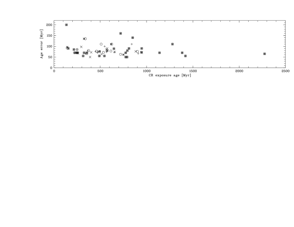
Figure 1: Datasets of CR exposure age and age error after application of the $<$100 Myr cleaning procedure. Results for the interval implementation, filtering from youngest to oldest age ($\times$, 42 points) and from oldest to youngest ($+$, 43 points), and the hierarchical implementation ($\circ$, 41 points)

4 Exposure age statistics

4.1 Distribution tests

The basic claim of S02/S03 was that a repeated clustering exists in the CR exposure age data at 143$\pm$10 Myrs period. They reason that the original dataset was cleaned to account for real age clustering and subsequently folded over the proposed 143 Myr period. This folded distribution was tested against a uniform distribution by a Kolmogorov-Smirnov (KS) test. The KS test measures the maximum distance $d$ between two cumulative distributions, and the KS statistics converts this into a probability that the one distribution has been randomly drawn from the test distribution (e.g., Press et al., 1995).

According to the test based on the KS statistics reported in S02/S03, the folded data distribution was a chance realisation when drawn from a uniform distribution with only 1.2% probability (identically for the two different datasets used in S02 and S03). This 1.2% probability was then interpreted as being a significant sign of a deviation from a uniform distribution and, with the folding step, that a periodic clustering of 143$\pm$10 Myrs was present in the data.

We have to note here that the KS test is most sensitive to differences around the mean of the distribution and less sensitive at the extreme ends (Press et al., 1995). In the case of periodic coordinates, as in the present case when considering the folded data, the phase zeropoint can be freely chosen to maximize the KS test signal. While S02/S03 did not comment on the phase zeropoint used, it did not lie exactly at $t=0$ Myrs and was likely shifted to achieve a maximum signal, which is a valid step.

To avoid this arbitrary shifting, it is useful to employ a variant of the KS statistics, the Kuiper statistics (e.g., Press et al., 1995; Stephens, 1970), that is an extension of the KS approach to circular coordinates. It is independent of the phase zeropoint of the independent coordinate, and thus more sensitive to a signal at any position compared to the KS test. Instead of the maximum distances $d$ between two cumulative distributions for the KS statistics, the Kuiper statistic is based on the sum $v$ of the maximum positive and negative distances between the two distributions. In the following we will use the Kuiper statistics and its measure $v$.

4.2 Effect of the age cleaning

When the cleaning procedure is applied to remove signatures of real age clustering (however physically appropriate), it does change the distribution of the data points. In the extreme case, if the data points were sampling the range of ages densely, the cleaning mechanism would result in exactly one data point every 100 Myrs for the interval implementation. For the hierarchical implementation the intervals would be larger, with a size depending on the age errors. In the real data the individual chemical groups only sparsely sample the age interval.

To assess the magnitude of this influence we perform Monte-Carlo simulations. We create random sets of 82 age points, uniformly drawn from an age range of 0–1001 Myr (7 full periods for 143 Myrs). We then assign to each ‘object’ age a random chemical group (out of the 11 present in the data), distributed as for the real data (1 to 20 per group). Then the two implementations of the cleaning procedure are applied as described above (only young-to-old for the interval implementation) and the dataset folded over a 143 Myr period. We repeat this 50 000 times each. For each realisation the Kuiper test against a uniform distribution is applied, to period-folded datasets both with and without cleaning. While the $v$ measure itself depends on the number of datapoints in a sample, the Kuiper probability statistics do not and, thus, the two resulting distributions of probabilities can be compared.

If the filter had no effect on the underlying distribution of datapoints, the resulting probabilities should reflect the random nature of the drawing process; i.e., the derived distribution of probabilities as given by the Kuiper statistics should again be uniform. In Figure 2 we plot the lowest 5% part of the cumulative distribution of the Kuiper test probabilities. 5% in this diagram means that in only 5% of random realisations a distribution as non-uniform as this should be drawn from a uniform distribution.

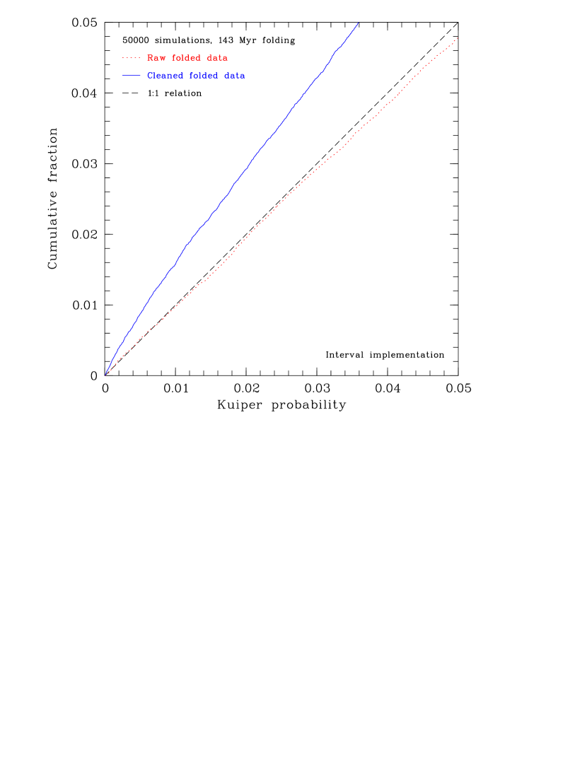
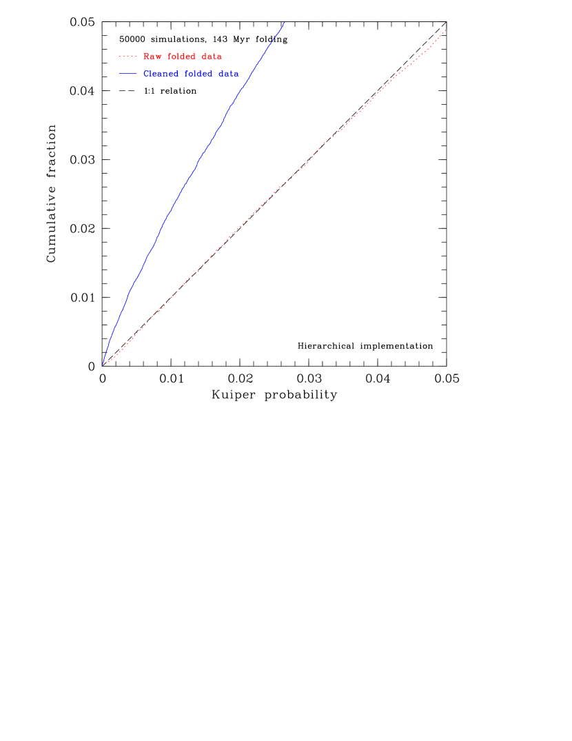
Figure 2: Cumulative distributions of the Kuiper statistic probabilities for 50 000 simulated datasets drawn from a uniform distribution, folded over a 143 Myrs period, and compared with a uniform distribution. Shown are the lowest, i.e., most significant 5%. Lines mark the raw, uncleaned (dotted line) and cleaned distributions (solid line). The dashed line marks the 1:1 limiting relation in the case of infinitely many simulations and no influence of the filtering on the distribution. Left: Interval implementation of the cleaning filter, right: hierarchical implementation.

For the raw, uncleaned distributions the probabilities lie as expected close to the 1:1 relation. Deviations are due to statistical noise and, to a small extend at the upper end, to the standard approximation formula used in computing probabilities from $v$ (Stephens, 1970). This is however not the case for the cleaned datasets, the probabilities given by the Kuiper test are systematically too low – for the hierarchical implementation even lower than for the interval implementation. This indicates that the distribution to compare against after cleaning and folding is not anymore a uniform distribution.

S02/S03 did not correct for this modified statistics, and if we assume this simulation to be valid also for their different use of age groups, their stated 1.2% would have to be changed to $\sim$3.7%. This is not a very high significance level anymore. For the interval implementation a 1.2% value is measured for $\sim$1.8% of the cases.

What this initial test shows primarily is that the simple comparison against a uniform distribution after cleaning and folding is not valid. In order to test against a uniform input distribution, the comparison distribution for a Kuiper test after cleaning and folding would need to be somewhat similar to a uniform distribution but its precise shape is not known. In the next section, we circumvent this problem by continuing to compare to a uniform distributions to compute the measure $v$, but we construct the distribution of probabilities for the $v$ values from simulations, and we do not use the Kuiper statistics directly.

5 Statistical tests on the original data

We want to study the probabilities that the two cleaned versions of literature data as given in Table On the periodic clustering of cosmic ray exposure ages of iron meteorites are drawn from a uniform distribution, after folding over a given period. This not only for a folding period of 143 Myr, but all periods ranging from 100 to 250 Myrs, to search for other periods with possibly significant signals. While this will result in a single probability for each period, we identified four factors that will result in an error bar on these probabilities: (1) the two different cleaning implementation, one with two cleaning directions; (2) the exact size of the cleaning interval; (3) the age errors associated with the data; and (4) number statistics.

5.1 $v$-statistics for the real data

For converting $v$ values into probabilities, we need to construct the Kuiper $v$ statistic for datasets with similar properties as the original data but drawn from a uniform distribution. While during larger parts of the interval 100–1000 Myrs the distribution appears to be rather uniform on larger scales, it clearly is not beyond 1000 Myrs (Figure 1). Therefore, as a basis for creating artificial datasets we construct an age density distribution that has a piecewise constant number density of meteorites, matched to that of the real data. This is shown in Figure 3. The intervals of constant number density have a size of $\geq$250 Myrs, which is at least as large as the largest folding period that we test here. The null hypothesis of the following tests is that the dataset is drawn from this distribution, after cleaning and folding. We now draw simulated datasets using a piecewise uniform distribution, with probabilites proportional to the local number density. This is identical to drawing random sets uniformly distributed in (0,1) and translate these values to ages using Figure 3.

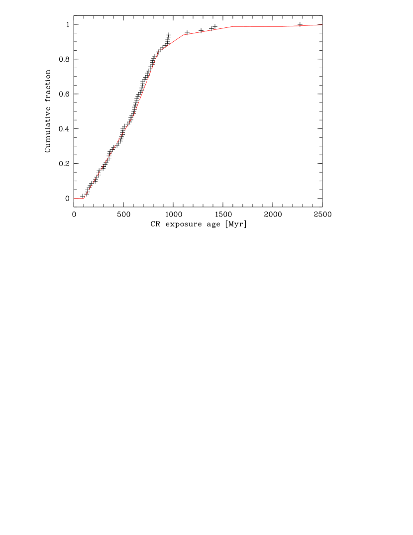
Figure 3: Construction of artificial datasets. Cumulative distributions of original data (symbols) and of function with $\geq$250 Myr piecewise constant probabilities matched to the data (line). From this function random datasets are drawn, with locally uniform distribution but this general distribution function.

Datasets constructed in such a way have values locally distributed uniformly, but follow the general density distribution on 250 Myr scales; in this way no local clusters are created. We then assign chemical classes to the 82 datapoints in each sample, with frequencies as in the real data.

5.2 Probabilities for cleaned data

We construct 2500 artificial datasets as described above and cleaned over a 100 Myr interval, fold each dataset over periods of 100–250 Myrs in 1 Myr steps, and compute the $v$ values when comparing to a uniform distribution. The same is done for the real data. This is repeated for the three variations of the cleaning filter for both real data and simulations. The comparison of $v$ for the real data with the $v$ statistics of the simulations determines the probabilities that the former is only a random realisation of the latter.

The resulting probabilities are shown in Figure 4, the three lines indicate the three cleaning variants. The relations deviate substantially for large parts of the period, showing differences between a few and $>$50 percent points. Over the full range the probabilities for all cleaning directions reach below 10% only around 162 Myrs.

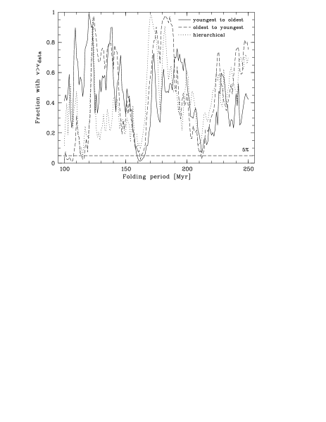
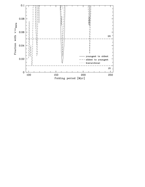
Figure 4: Probabilities that the period-folded data are drawn from a uniform distribution, as a function of folding period and without any error bars. Shown are the full range of periods (100–250 Myrs) and full range of probabilities (left) and the most significant 10% probabilities as a zoom (right). The three lines correspond to the two interval cleaning variants, youngest to oldest (solid line) and oldest to youngest age (dashed line), the dotted line to the hierarchical cleaning (dotted line). Horizontal lines mark the 95 and 99% significance levels, respectively.

6 Sources of uncertainty

While in Figure 4 already the influence of the different cleaning implementation is indicated, the next step is to construct error bars on the probabilities reflecting also the other three sources or error. We make the assumption that these are at maximum weakly dependent on each other, and treat them separately.

6.1 Size of the cleaning interval

So far we used the cleaning interval size of 100 Myrs as suggested by S02/S03. However 100 has a single significant figure – the value is not 100.0 – which seems adequate since the value stems from a rough estimate in Voshage & Feldmann (1979). For this reason we study the dependence of probabilites on the exact interval size. We vary it by 10%, so using also 90 and 110 Myrs.

With these interval sizes we repeat the analysis from Section 5.2 above, again creating 2500 simulated datasets and computing the $v$ statistics for simulations and real data. We do this for the young to old interval cleaning and the hierarchical cleaning. As shown in Figure 5, the results exhibit a spread between the three models of similar size as for the use of different cleaning implementations.

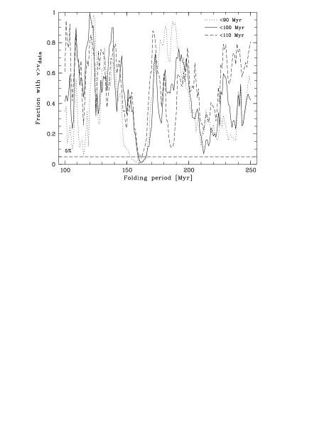
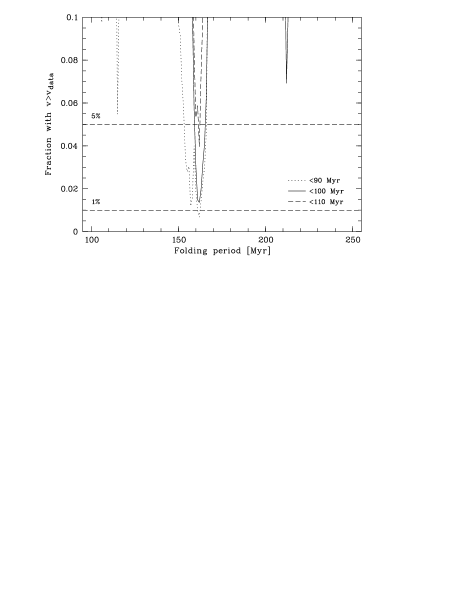
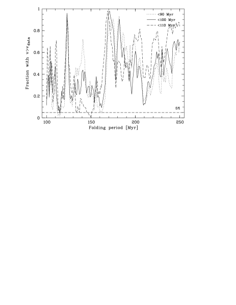
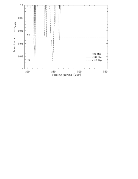
Figure 5: Similar to Figure 4 but for three cleaning interval sizes: 90 Myrs (dotted line), 100 Myrs (solid line, as in Figures 4), and 110 Myrs (dashed line). Top: interval cleaning from youngest to oldest age; bottom: hierarchical cleaning.

6.2 Age uncertainties

The age uncertainties were neglected up to now. The errors in age originally quoted by Voshage & Feldmann (1979) and Voshage et al. (1983) lie in the range $50<\sigma(t)<230$ Myr, and after the 100 Myr cleaning at $50<\sigma(t_{\mathrm{100}})<200$ Myr. However, in a discussion of the strength of the clustering signal, S03 claimed an “at most 30 Myrs” uncertainty in the ages, estimated from “comparing the potassium ages to ages determined using other methods”. While he did not give a reference for this claim there, he likely refered to Lavielle et al. (1999). That study showed substantially different CR exposure ages using ³⁶Cl, ³⁶Ar, and ¹⁰Be measurements instead of $K$ for 13 meteorites. When following the conclusions in Lavielle et al. (1999) of an increase in CR flux over the last $\sim$10 Myrs, the ages from the two isotope methods can be brought into better agreement and a comparison delivers age uncertainties from comparing $K$ and ¹⁰Be ages of rather 10–70 Myrs than 50–230 Myrs as in Voshage & Feldmann (1979) and Voshage et al. (1983).

In S03 it was noted that “the error will have the tendency to smear the distribution”. This is an important point in the light that S02/S03 disregarded the errors in the analysis altogether and did not test their influence on the results.

While we again can not and do not attempt to determine ‘real’ age uncertainties, we want to assess the contribution to probability error bars from different models of age uncertainties. We again use simulation to create a statistic of $v$ values. Here we assume two error models in addition to the ‘no errors’ in Section 5.2: (a) the originally published errors, and (b) 30 Myr errors for all data points. We again create 2500 datasets each, assuming the errors to be gaussian, age-clean (100 Myr), and fold them to derive the $v$ statistics for these sets. The results are shown in Figure 6, similar to Figure 4. The chance realisation for a null hypothesis increases by a small amount for the original errors compared to the 30 Myr errors or the case without errors. In comparison to other sources of uncertainty, the effect of age errors is in fact negligible.

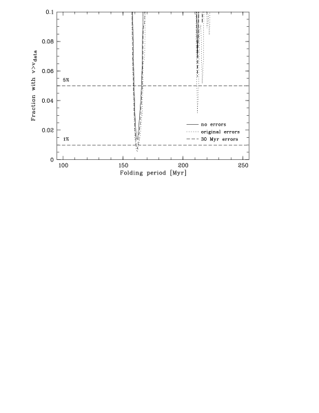
Figure 6: As Figure 4 but for different assumed age uncertainty models. Data are interval cleaned (young to old, 100 Myr). Shown are the probabilities in case of no errors (solid line, as in Figures 4), original errors (dotted line), and assumed 30 Myr errors for all objects (dashed line).

6.3 Number statistics

The last source of error we study here is the influence of number statistics on random clustering in the real data. With $\sim$40 datapoints in the dataset after cleaning, each individual point has a non-negligible influence on the statistics.

So far, the $v$ distribution from simulated datasets shows the effect of different discrete random realisations of the null hypothesis. However, the simulation do not make statements about the influence of number statistics from the data side. We need to quantify how strongly an apparently significant deviation from the null hypothesis might be depending on a single or a few data points, i.e., statistical outliers.

For this application the statistical method of bootstrap simulations has been shown to be a valid approach (see Press et al., 1995, and references therein), given that the data are independent and identically distributed. Even though this is not strictly the case here after the application of the cleaning filter, the interdependences of datapoints are both rather local and weak. We thus assume that this has only a negligible influence, which allows us to perform a bootstrap of the data.

The bootstrap allows the estimation of error bars for a certain parameter from a measured dataset itself. New datasets with the same size as the original are drawn from the original dataset with replacements. The parameter in question is then determined from the bootstrapped datasets as before and the spread in this parameter is a good estimate for its uncertainty.

Here we use bootstrapping to estimate the influence of number statistics on the $v$ value for our data. $v$ is a valid parameter with which to apply bootstrapping, but with the follwoing caveat: the $v$ statistics gets skewed by the bootstrapping process itself, as a result of some datapoints being present more than once in the bootstrapped datasets. This changes the cumulative distributions to be less smooth, and thus skewes the $v$ statistics towards higher values.

For this reason we construct bootstrapped datasets from our data and compare these to bootstrapped datasets of simulations. In this way the same modification is applied to both sides, and $v$ can again be compared. We create 2500 bootstrapped simulation for this case, applying the bootstrapping after cleaning. The dataset is also cleaned with a 100 Myr interval (interval implementation, younger to older ages, and hierarchical implementation), and then bootstrapped 500 times. We fold the distributions over 100–250 Myr periods, and receive a $v$ statistic for each period given the null hypothesis. By comparing the $v$ statistics from the bootstrap realisations of the real data to that of the simulations we get a distribution of probabilities that the measured $v$ is larger than the random simulated $v$. We show the median and upper and lower quartiles in Figure 7.

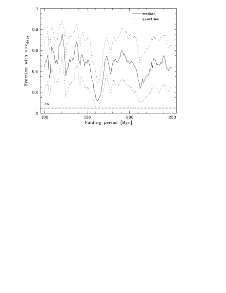
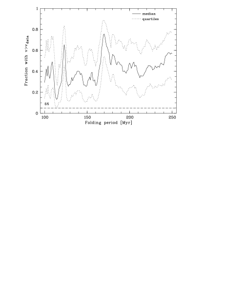
Figure 7: Distribution of probabilities from bootstrapping of the 100 Myr interval cleaned dataset, cleaned younger to older ages (left) and hierarchical cleaning (right). Shown are the median (solid line) and upper and lower quartiles (dotted lines) of the probabilities. As a result of number statistics no period has a significant signal for deviation from a uniform distribution.

The lower quartile drops to $\sim$5% around 162 Myrs for the interval implementation, and for the hierarchical implementation around 114 Myrs. For no period in both implementaions the median drops below the 10% mark. This indicates that in the tests above only a few outlying datapoints are responsible for the probabilities below 5%.

7 Discussion

Simple statistical tests against a uniform distribution do not tell the whole truth about the clustering properties of the dataset of meteorite CR exposure ages. It is obvious from Figure 4 that the exact implementation of the cleaning mechanism can already have a strong influence on the composition of the dataset.

A similar case is the influence of the exact choice of the cleaning interval (Figure 5). There is no good argument available from S02/S03 or the referenced literature why more than one significant figure for the ‘100’-Myr interval should be assumed. Thus 90 and 110 Myrs are valid variations – 80 and 120 Myrs would be, too – with the substantial influence on the resulting probabilities seen above. In comparison, the influence of the age uncertainties using different age uncertainty models (Figure 6) is small compared to the first two sources.

In Figure 8 we show the probabilities for a total of 27 different combinations of cleaning implementation, cleaning interval size, and error model, expored by simulations. The used combinations are listed in Table 1. The existence of such variations is a consequence of the fact that an inherent clustering of real meteorite ages as a difference to CR exposure ages has to be removed from the input data to allow a conversion of exposure age distribution to CR flux levels. A filtering procedure for this fact is not uniquely defined.

If the variations we make are valid, and the arguments given above suggest so, then the spread seen in the probabilities for a given period is a good indicator how significant the signal for a given folding period is at maximum – neglecting the influence of number statistics for now. From Figure 8 it is clear that there exists no significant signal for a deviation from a uniform distribution of ages for a period of $\sim$143 Myrs. In only three of the 27 cases the probabilities for a random realisation drops below 10%, in none below 5%. At a period of 150 Myrs there are six combinations that give probabilities of around 1%. However, the remaining 21 are at $>$10% and thus not significant. The only periods that give low values lie around 162 Myrs.

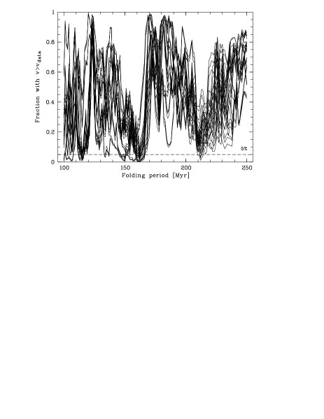
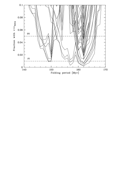
Figure 8: As Figure 4 but for the 27 different combinations of cleaning implementation, cleaning interval size, and error model in Table 1. Left: Full range of periods from 100 to 20 Myrs. Right: Zoom on region around 143 and 162 Myr, showing the top 10% probabilities.

We summarized the probabilities for the 162 Myr period in Table 1. While for this period there are several parameter combinations that result in probabilities below 1%, there are also others that are above 2.5, 5, and even 10%. If there are no strong arguments against these combinations as being valid, then also the 162 Myr period clearly disqualifies as showing a significant signal for being different from a uniform distribution. At other periods there are also some of the parameter combinations with probabilities below 5% that are countered by combinations with above 10% probability.

Table 1: Probabilities for a deviation from a uniform distribution when folding at 162 Myrs, while neglecting the influence of number statistics. Given are the probabilities for different cleaning implementations (interval young to old, old to young ages, and hierarchical), exact sizes of the cleaning interval (90, 100, 110 Myrs), and the assumed error model for the ages (no errors, 30 Myr errors, original errors).

Cleaning	Interval: young to old			Interval: old to young			Hierarchical
Error model	90 Myr	100 Myr	110 Myr	90 Myr	100 Myr	110 Myr	90 Myr	100 Myr	110 Myr
no errors	0.68%	1.4%	4.0%	6.4%	2.4%	7.8%	4.5%	9.4%	27.8%
30 Myrs	0.32%	0.72%	2.3%	4.5%	1.8%	5.7%	2.7%	6.9%	23.9%
original errors	0.20%	0.52%	2.0%	3.6%	1.2%	4.6%	1.8%	5.1%	22.1%

Into this interpretation one additional factor enters: number statistics. Figure 7 demonstrates the span of probabilities that is induced by number statistics, as tested by bootstrap simulations. For the simulations we used both the 100 Myr interval and hierarchical cleaning, and absence of errors. For a different choice of the other parameters we expect some shifts in this distribution, but no dramatic changes. The spread in probabilities in Figure 7 (shown are median and quartiles) is a direct expression of small number statistics in the data. For the shown cases we have 42 and 41 data points in the sample after cleaning. With increasing number of data points this spread should decrease. So in order to decrease this to a range that allows detection of only 1% probability, at the given strength of potential signals, the dataset has to be larger by, say, at least an order of magnitude.

In conclusion, we see no signal of periodic clustering with any period between 100 and 250 Myrs for the dataset of 82 iron (including one stony-iron) meteorites. For all periods the dataset of CR exposure ages is consistent with being drawn from a uniform distribution of ages after cleaning for multiple-breakup clusters. This conclusion holds when including all discussed error sources, and even when incorrectly neglecting the effects of number statistics.

Why are these results differing so strongly from S02/S03? We identify three main resons:

• The implementation of the cluster cleaning filter is clearly different between S02/S03 and this study, by using a different chemical grouping scheme. However, there is agreement in meteoritics on the current 14 group classification (plus possible further extentions). In any case this allows meteorites (e.g., from the former IIIA and IIIB groups) to originate from the same parent body in the same break-up event, which has to be recognised in the cleaning process. This leaves us with less chemical groups and hence less data points after cleaning, compared to S02/S03.

• S02/S03 did not test the influence of the cleaning process on the statistical properties of their dataset. This led to a skewed statistic and falsly too low probability values even for their original method.

• In S02/S03 no check of the influence of error sources on the face-value results of the KS-test was done. In particular, they did not test the influence of the relative importance – from small number statistics – of individual datapoints on their results. This together resulted in an substantial over-interpretation of their result as being significant.

These statements are made from a statistical side. We want to make clear that there are other issues that we did not touch, e.g., whether the proposed filter against intrinsic meteorite breakup clustering is sufficient and thus useful. Residuals of intrinsic meteorite clustering would of course strongly influence the detection of CR exposure age clustering. Especially if the sought periodicity of 143 Myrs is only a factor of $\sim$1.4 longer than the proposed real clustering length.

8 Conclusions

We have investigated the claim by S02/S03 that a sample of $\sim$80 iron meteorites showed a CR exposure age distribution with a 143$\pm$10 Myr periodic clustering over the last 1–2 Gyrs. From this they concluded a periodicity in the CR influx from different amounts of star formation during the solar system’s passage through the spiral arms of our galaxy.

We followed their approach and computed the probability that the data are drawn from a uniform distribution of ages, when folded over the proposed period. As a difference to S02/S03 we studied several sources that create uncertainties in the derived probabilities, and tested the influence of filtering of their data, by using simulations.

The data are ‘cleaned’ from real age clusters from breakups of meteoroids into multiple pieces – as suggested by S02/S03. As a side result we find that such a filter can be implemented in several ways, with all implementations having special advantages and disadvantages. Computing the probabilities of the data as random realisations of a uniform distribution we see a minimum at a period of 162 Myrs, and clearly not at 143 Myrs. When assessing the influence of different sources of uncertainty, we compare the probabilities for a random realisation for this 162 Myr period. When neglecting the influence of number statistics to study the effects of the different error sources, we find a non-negligible influence of (i) the implementation of the age filtering, (ii) the exact choice of the size of the cleaning interval, and (iii) to a smaller amount the influence of different assumed age error models.

However, this is with the neglection of noise from number statistics. There is no folding period with a consistent probability for a random realisation of a uniform distribution of below 5%, when considering the above error sources, including 143 and 162 Myrs period.

On top of this, number statistics is clearly the strongest source of influence, larger than the three sources above. Noise from small number statistics – $\sim$40 data points in the sample after cleaning – creates a scatter in the probability of the data, being a random realisation of an underlying distribution. For any folding period from 100 to 250 Myrs $\ga$75% of the corresponding bootstrap realisations created for the dataset deliver probabilities for a random draw from a uniform distribution of 5% or higher, including the 143 and 162 Myr periods. Thus, there is no period between 100 and 250 Myrs at which the folded age distribution of the dataset is inconsistent with being drawn from a uniform distribution. With the data and the methods proposed by S02/S03 no periodic variation of the cosmic CR background is found.

The differences of interpretation in S02/S03 to our results are due to: (i) the use of an outdated chemical classification scheme, (ii) the neglection of the influence of the filtering against real age clusters on the KS statistics, and (iii) the neglection of error sources, including number statistics, on the significance of the results.

[x]lllllllllll Data base of meteorite CR exposure ages. Given are name of meteorite, chemical group (original group in parentheses, see text), data source (V79 for Voshage & Feldmann (1979), V83 for Voshage et al. (1983)), CR exposure age $t$, error in exposure age $\sigma(t)$. $t_{\mathrm{100,+}}$, $\sigma(t_{\mathrm{100}},+)$, $t_{\mathrm{100,-}}$, and $\sigma(t_{\mathrm{100}},-)$ are values after combining meteorites within $\Delta(t)<100$ Myr of age, ‘+’ combining intervals with increasing age, ‘–’ with decreasing ages. $t_{\mathrm{H}}$ and $\sigma(t_{\mathrm{H}})$ correspond to values computed with the hierarchical filter used in S02/S03. The triangles mark entries that have been combined to the value given below ($\bigtriangledown$) or above ($\bigtriangleup$), respectively. Meteorites with suffix ‘-An’ have an anomalous chemical composition.
Name GroupSource $t$ $\sigma(t)$ $t_{\mathrm{100,+}}$ $\sigma(t_{\mathrm{100,+}})$ $t_{\mathrm{100,-}}$ $\sigma(t_{\mathrm{100,-}})$ $t_{\mathrm{H}}$ $\sigma(t_{\mathrm{H}})$
continued.
Name GroupSource $t$ $\sigma(t)$ $t_{\mathrm{100,+}}$ $\sigma(t_{\mathrm{100,+}})$ $t_{\mathrm{100,-}}$ $\sigma(t_{\mathrm{100,-}})$ $t_{\mathrm{H}}$ $\sigma(t_{\mathrm{H}})$
Morradal An V79 155 90 155 90 155 90 155 90
South Byron An V79 255 70 255 70 255 70 255 70
Washington County An V79 575 80 575 80 575 80 575 80
Pinon An V79 790 50 790 50 790 50 790 50
Deep Springs An V79 2275 65 2275 65 2275 65 2275 65
Surprise Springs IAB (IA) V83 130 170 $\bigtriangledown$$\bigtriangledown$ 135 200 134 200
Bohumilitz IAB (IA) V79 140 230 135200 $\bigtriangleup$ $\bigtriangleup$ $\bigtriangleup$ $\bigtriangleup$
Rifle IAB (IA) V79 490 70 $\bigtriangledown$$\bigtriangledown$ 493 77 493 75
Mayerthorpe IAB (IA) V79 495 105 $\bigtriangledown$$\bigtriangledown$ $\bigtriangleup$ $\bigtriangleup$ $\bigtriangleup$ $\bigtriangleup$
Osseo IAB (IA) V79 495 55 493 77 $\bigtriangleup$ $\bigtriangleup$ $\bigtriangleup$ $\bigtriangleup$
Canyon Diablo IAB (IA) V79 645 103 $\bigtriangledown$$\bigtriangledown$ 648 89 648 89
Bogou IAB (IA) V79 650 75 648 89 $\bigtriangleup$ $\bigtriangleup$ $\bigtriangleup$ $\bigtriangleup$
Balfour Downs IAB (IA) V79 840 110 $\bigtriangledown$$\bigtriangledown$ 840 110 902 76
Odessa IAB (IA) V79 875 70 $\bigtriangledown$$\bigtriangledown$ 910 66 $\bigtriangleup$ $\bigtriangleup$
Bischtuebe IAB (IA) V79 895 75 $\bigtriangledown$$\bigtriangledown$ $\bigtriangleup$ $\bigtriangleup$ $\bigtriangleup$ $\bigtriangleup$
Yardymly Aroos IAB (IA) V79 920 50 882 76 $\bigtriangleup$ $\bigtriangleup$ $\bigtriangleup$ $\bigtriangleup$
Mount Ayliff IAB (IA) V79 950 70 950 70 $\bigtriangleup$ $\bigtriangleup$ $\bigtriangleup$ $\bigtriangleup$
Deport IAB (IA) V79 1140 70 1140 70 1140 70 1140 70
Nocoleche IC V79 250 70 250 70 250 70 250 70
Bedego IC V79 940 90 $\bigtriangledown$$\bigtriangledown$ 948 90 947 90
Arispe IC-An V79 955 90 948 90 $\bigtriangleup$ $\bigtriangleup$ $\bigtriangleup$ $\bigtriangleup$
Smithonia IIAB (IIA) V79 90 80 $\bigtriangledown$$\bigtriangledown$ 144 96 142 92
Sierra Gorda IIAB (IIA) V79 140 110 $\bigtriangledown$$\bigtriangledown$ $\bigtriangleup$ $\bigtriangleup$ $\bigtriangleup$ $\bigtriangleup$
El Burro IIAB (IIB) V79 165 115 $\bigtriangledown$$\bigtriangledown$ $\bigtriangleup$ $\bigtriangleup$ $\bigtriangleup$ $\bigtriangleup$
Cedartown IIAB (IIA) V79 180 80 144 96 $\bigtriangleup$ $\bigtriangleup$ $\bigtriangleup$ $\bigtriangleup$
Lombard IIAB (IIA) V79 295 200 $\bigtriangledown$$\bigtriangledown$ 325 135 339 135
Sikhote Alin IIAB (IIB-An) V79 355 70 325135 $\bigtriangleup$ $\bigtriangleup$ $\bigtriangleup$ $\bigtriangleup$
Calico Rock IIAB (IIA) V83 545 55 545 55 545 55 545 55
Sandia Mountains IIAB (IIB) V79 720 160 720160 720 160 720 160
Ainsworth IIAB (IIB) V79 1280 110 1280110 1280 110 1280 110
Wiley IIC-An V79 810 90 810 90 810 90 810 90
Unter Mässing IIC V83 1385 70 1385 70 1385 70 1385 70
Brownfield IID V79 355 70 355 70 355 70 355 70
Carbo IID V79 850 140 850140 850 140 850 140
Sacramento Mountains IIIAB (IIIA) V79 315 55 315 55 315 55 315 55
Descubridora Charkas IIIAB (IIIA) V79 510 110 $\bigtriangledown$$\bigtriangledown$ 548 100 510 110
Sanderson IIIAB (IIIB) V79 585 90 $\bigtriangledown$$\bigtriangledown$ $\bigtriangleup$ $\bigtriangleup$ 615 78
Trenton IIIAB (IIIA) V79 605 60 567 87 652 73 $\bigtriangleup$ $\bigtriangleup$
San Angelo IIIAB (IIIA) V79 610 80 $\bigtriangledown$$\bigtriangledown$ $\bigtriangleup$ $\bigtriangleup$ $\bigtriangleup$ $\bigtriangleup$
Tamarugal IIIAB (IIIA) V79 610 85 $\bigtriangledown$$\bigtriangledown$ $\bigtriangleup$ $\bigtriangleup$ $\bigtriangleup$ $\bigtriangleup$
Treysa IIIAB (IIIB-An)V79 620 60 $\bigtriangledown$$\bigtriangledown$ $\bigtriangleup$ $\bigtriangleup$ $\bigtriangleup$ $\bigtriangleup$
Merceditas IIIAB (IIIA) V79 625 80 $\bigtriangledown$$\bigtriangledown$ $\bigtriangleup$ $\bigtriangleup$ $\bigtriangleup$ $\bigtriangleup$
Picacho IIIAB (IIIA) V83 635 50 $\bigtriangledown$$\bigtriangledown$ $\bigtriangleup$ $\bigtriangleup$ $\bigtriangleup$ $\bigtriangleup$
Lenarto IIIAB (IIIA) V79 670 80 $\bigtriangledown$$\bigtriangledown$ $\bigtriangleup$ $\bigtriangleup$ 719 63
Gundaring IIIAB (IIIA) V79 685 90 $\bigtriangledown$$\bigtriangledown$ $\bigtriangleup$ $\bigtriangleup$ $\bigtriangleup$ $\bigtriangleup$
Joe Wright Mts IIIAB (IIIB) V83 685 70 $\bigtriangledown$$\bigtriangledown$ $\bigtriangleup$ $\bigtriangleup$ $\bigtriangleup$ $\bigtriangleup$
Puende del Zacate IIIAB (IIIA) V79 690 85 $\bigtriangledown$$\bigtriangledown$ $\bigtriangleup$ $\bigtriangleup$ $\bigtriangleup$ $\bigtriangleup$
Norfolk IIIAB (IIIA) V79 695 67 $\bigtriangledown$$\bigtriangledown$ $\bigtriangleup$ $\bigtriangleup$ $\bigtriangleup$ $\bigtriangleup$
Grant IIIAB (IIIB) V79 695 65 656 74 $\bigtriangleup$ $\bigtriangleup$ $\bigtriangleup$ $\bigtriangleup$
Mount Edith IIIAB (IIIB) V79 715 65 $\bigtriangledown$$\bigtriangledown$ 750 61 $\bigtriangleup$ $\bigtriangleup$
Santa Apolonia IIIAB (IIIA) V79 740 65 $\bigtriangledown$$\bigtriangledown$ $\bigtriangleup$ $\bigtriangleup$ $\bigtriangleup$ $\bigtriangleup$
Williamstown IIIAB (IIIA) V79 740 55 $\bigtriangledown$$\bigtriangledown$ $\bigtriangleup$ $\bigtriangleup$ $\bigtriangleup$ $\bigtriangleup$
Thunda IIIAB (IIIA) V79 755 60 $\bigtriangledown$$\bigtriangledown$ $\bigtriangleup$ $\bigtriangleup$ $\bigtriangleup$ $\bigtriangleup$
Delegate IIIAB (IIIB-An)V79 800 60 750 61 $\bigtriangleup$ $\bigtriangleup$ $\bigtriangleup$ $\bigtriangleup$
Dayton IIICD (IIID) V79 215 85 215 85 215 85 215 85
Anoka IIICD (IIIC) V79 600 150 $\bigtriangledown$$\bigtriangledown$ 618 110 624 110
Carlton IIICD (IIIC) V79 635 70 618110 $\bigtriangleup$ $\bigtriangleup$ $\bigtriangleup$ $\bigtriangleup$
Mundingi IIICD (IIIC) V79 790 100 $\bigtriangledown$$\bigtriangledown$ 792 80 793 80
Edmonton (KY) IIICD (IIICD-An)V83 795 60 792 80 $\bigtriangleup$ $\bigtriangleup$ $\bigtriangleup$ $\bigtriangleup$
Rhine Villa IIIE V83 325 70 325 70 325 70 325 70
Kokstad IIIE V83 470 70 $\bigtriangledown$$\bigtriangledown$ 470 70 534 72
Willow Creek IIIE V83 560 57 515 64 568 74 $\bigtriangleup$ $\bigtriangleup$
Coopertown IIIE V83 575 90 575 90 $\bigtriangleup$ $\bigtriangleup$ $\bigtriangleup$ $\bigtriangleup$
Nelson County IIIF V79 490 55 490 55 490 55 490 55
Clark County IIIF V79 1420 55 1420 55 1420 55 1420 55
Duchesne IVA V79 220 70 $\bigtriangledown$$\bigtriangledown$ 220 70 220 70
Yanhuitlan IVA V79 300 65 260 68 342 65 355 66
Seneca Township IVA V79 360 50 $\bigtriangledown$$\bigtriangledown$ $\bigtriangleup$ $\bigtriangleup$ $\bigtriangleup$ $\bigtriangleup$
Charlotte IVA V79 365 80 $\bigtriangledown$$\bigtriangledown$ $\bigtriangleup$ $\bigtriangleup$ $\bigtriangleup$ $\bigtriangleup$
Iron River IVA V79 400 70 $\bigtriangledown$$\bigtriangledown$ 448 76 $\bigtriangleup$ $\bigtriangleup$
Putnam County IVA V79 435 70 $\bigtriangledown$$\bigtriangledown$ $\bigtriangleup$ $\bigtriangleup$ 461 78
Huizopa IVA V79 450 90 402 72 $\bigtriangleup$ $\bigtriangleup$ $\bigtriangleup$ $\bigtriangleup$
Hill City IVA V79 475 90 $\bigtriangledown$$\bigtriangledown$ $\bigtriangleup$ $\bigtriangleup$ $\bigtriangleup$ $\bigtriangleup$
Bristol IVA V79 480 60 478 75 $\bigtriangleup$ $\bigtriangleup$ $\bigtriangleup$ $\bigtriangleup$
Maria Elena IVA V79 775 50 775 50 775 50 775 50
Tawallah Valley IVB V79 250 85 $\bigtriangledown$$\bigtriangledown$ 250 85 250 85
Hoba IVB V79 340 110 295 98 365 80 374 80
Weaver Montains IVB V79 390 50 390 50 $\bigtriangleup$ $\bigtriangleup$ $\bigtriangleup$ $\bigtriangleup$
Cape of Good Hope IVB V79 775 70 775 70 775 70 775 70
Tlacotepec IVB V79 945 55 $\bigtriangledown$$\bigtriangledown$ 945 72 945 73
Skookum Klondige IVB V79 945 90 945 72 $\bigtriangleup$ $\bigtriangleup$ $\bigtriangleup$ $\bigtriangleup$
Glorieta Mountains PAL V79 230 70 230 70 230 70 230 70