On the He II Emission In $\eta$ Carinae and the Origin of Its Spectroscopic Events

Abstract

We describe and analyze Hubble Space Telescope (HST) observations of transient emission near 4680 Å in $\eta$ Car, reported earlier by Steiner & Damineli (2004). If, as seems probable, this is He II $\lambda$4687, then it is a unique clue to $\eta$ Car’s 5.5-year cycle. According to our analysis, several aspects of this feature support a mass-ejection model of the observed spectroscopic events, and not an eclipse model. The He II emission appeared in early 2003, grew to a brief maximum during the 2003.5 spectroscopic event, and then abruptly disappeared. It did not appear in any other HST spectra before or after the event. The peak brightness was larger than previously reported, and is difficult to explain even if one allows for an uncertainty factor of order 3. The stellar wind must provide a temporary larger-than-normal energy supply, and we describe a special form of radiative amplification that may also be needed. These characteristics are consistent with a class of mass-ejection or wind-disturbance scenarios, which have implications for the physical structure and stability of $\eta$ Car.

1 Introduction

Steiner & Damineli (2004) reported He II $\lambda$4687 emission in ground-based spectra of $\eta$ Carinae. Since He II represents a far higher excitation or ionization state than other lines normally seen in this object, it may be a valuable clue to $\eta$ Car’s mysterious 5.5-year cycle and to the structure of strong shock fronts in the extraordinary stellar wind (see refs. cited below). Here we report observations of the same feature with higher spatial resolution and other advantages using the Space Telescope Imaging Spectrograph (HST/STIS). We find:

• During the first half of 2003, broad emission appeared between 4675 Å and 4695 Å. It peaked at the time of the mid-2003 “spectroscopic event,” with a maximum equivalent width close to 2.4 Å. He II $\lambda$4687 is the probable identification.

• The emission was not spatially resolved from the central star. Therefore it originated in the dense stellar wind, not in diffuse ejecta at larger radii.

• This feature was not present in any HST/STIS observation before 2003.0, nor after 2003.5, with a 1-sigma detection limit of about 40 mÅ for each occasion and 15 mÅ for the average.

• Our measurement of the peak brightness considerably exceeds the value reported by Steiner & Damineli. The main source of disagreement is explained in Section 5 below.

• Even if one adopts the lower flux estimate, He II $\lambda$4687 became far too bright to explain with a conventional model. The hypothetical companion star’s wind cannot supply enough energy for the required shock fronts. The observed emission probably required a mass ejection event on the primary star, and/or some special radiative processes described in Section 8 below.

• Regarding the nature of the spectroscopic event, several aspects of the He II emission all support a mass-ejection or wind-disturbance type of model. The observed behavior presents severe difficulties for an “eclipse” scenario.

These conclusions are justified in Sections 3–9 below. Qualitatively, one expects shock fronts near Eta Carinae to produce weak He II emission; but quantitatively the observed flux presents a difficult energy-supply problem. Either the deduced intrinsic strength is in error for reasons unknown, or some extraordinary process occurred during the 2003 spectroscopic event.

Since the late 1940’s, $\eta$ Car has undergone periodic spectroscopic events characterized by the disappearance of high-excitation lines such as He I and [Ne III], both in the stellar wind and in its nearby slow ejecta. Zanella et al. (1984) conjectured that these are essentially mass-ejection episodes. They recur with a period of 5.5 years (Damineli, 1996; Whitelock et al., 1994), and the emission feature analyzed in this paper was obviously correlated with the event that occurred in mid-2003.

As noted by Steiner and Damineli and discussed below, the He II emission problem probably involves X-rays, which vary systematically. Preceding a spectroscopic event, $\eta$ Car’s observable 2–10 keV hard X-ray flux rises, becoming increasingly unstable or chaotic, and then crashes almost to zero (Ishibashi et al., 1999; Corcoran, 2005). Softer X-rays, which are crucial for our discussion, may behave quite differently but cannot be observed because they are absorbed by intervening material. The most common explanation for $\eta$ Car’s X-ray production is a colliding-wind binary model. Some authors believe that each 5.5-year event involves an eclipse of a hot secondary star by the primary wind (e.g., see Pittard & Corcoran (2002)) – instead of a mass ejection event, or, perhaps, in addition to it. On the other hand, a mass-ejection model, either binary or single-star, does not require an eclipse (Davidson, 1999, 2002). The hypothetical companion star has not been detected, nor have Doppler velocities in the primary wind provided a valid orbit (Davidson et al., 2000). The two alternative scenarios, eclipse vs. mass-ejection, differ in fundamental significance because the former is simply a result of geometry but the latter requires an undiagnosed stellar surface instability; see remarks in Davidson (2002, 2005b).

So far as we know, Gaviola (1953) reported the earliest suspected detection of He II $\lambda$4687 in $\eta$ Car. He listed two separate emission features near 4680 Å and 4686 Å that were comparable in strength to He I $\lambda$4714. According to the notes in his paper, each of them appeared only in one observation during the interval from April 1944 through March 1951. Gaviola obtained data during a spectroscopic event in 1948 but understandably he did not recognize it as such, and his notes do not state whether that was the time when the emission in question appeared. If he observed emission at 4686 Å on one occasion in 1948 and then 4680 Å somewhat later, the wavelength shift would resemble that which occurred in 2003 (see Section 6). Unfortunately the published record does not state whether this was the case, and it is possible that Gaviola’s spectra showing this emission feature did not correspond to a spectroscopic event (see below).

Thackeray (1953) reported that a weak feature occurred near 4687 Å at some time between April 1951 and June 1952. Feast (2004, private communication), examining Thackeray’s plates, confirms that such emission may have been present on 1951 June 14 and 1951 July 10. In itself this evidence is weak, since Thackeray and Feast both expressed doubt and the observations did not coincide with an “event” in the 5.5-year cycle. However, we note that 1951 was an unusual period in $\eta$ Car’s recovery from its Great Eruption. He I and other moderately high-excitation emission had first appeared only a few years earlier (Feast et al., 2001; Humphreys & Koppelman, 2005; Gaviola, 1953), and the star brightened rapidly during the same era (O’Connell, 1956; de Vaucouleurs & Eggen, 1952). Thus its wind may have changed from one state to another in the years preceding 1953; see Martin (2005), Davidson et al. (2005a), Davidson (2005b), and refs. cited therein. Thus we should not dismiss the possibility that Thackeray’s plates really did show He II $\lambda$4687 in 1951.

Since the Hubble Treasury Project for $\eta$ Carinae was intended primarily to observe the spectroscopic event in 2003, we obtained STIS data repeatedly during that year. Similar observations had been made on a few earlier occasions from 1998 to 2002. In this paper we discuss emission near 4680 Å in the STIS data; we also note some pertinent ground-based VLT/ESO observations, see Stahl et al. (2005). Often we refer to the feature in question as “4680 Å,” its approximate peak wavelength at maximum strength, because it is quite broad and in principle the He II identification has not been fully confirmed. (See Section 4.) We also present a theoretical assessment of the energy budget implied by the line’s strength, which appears almost paradoxical. In general, we shall conclude that the observations favor a mass-ejection or wind-disturbance scenario, consistent with suggestions by Zanella et al. (1984), Davidson (1999), Davidson (2002), and Smith et al. (2003); and that an eclipse does not explain the He II problem.

We describe the observations in Section 2, the observational constraints on the spatial extent of the emitting region in Section 3, identification of the feature in Section 4, the emission strength and behavior in Sections 5 and 6, the theoretical problem in Section 7 and 8, and – most important– a summary of implications in Section 9. A number of technical details and equations are presented in separate Appendixes.

2 STIS CCD Data

The main spectra in this paper were obtained as part of the $\eta$ Carinae HST Treasury Project (Davidson, 2004a) and were reduced using a modified version of the Goddard CALSTIS reduction pipeline. The modified pipeline uses the normal HST bias subtraction, flat fielding, and cosmic ray rejection procedures with the addition of improved pixel interpolation and improved bad/hot pixel removal. Information regarding these modifications can be found online at our web site and in a forthcoming publication (Davidson et al., in preparation). Each one-dimensional STIS spectrum discussed here is essentially a 0.1″ $\times$ 0.25″ spatial sample: the pixel size was 0.05″, the slit width was about 2 CCD columns, and each spectral extraction sampled 5 CCD rows. Complex details of our pixel interpolation methods, etc., do not materially affect these results. The CCD column width corresponded to a wavelength interval of about 0.28 Å or 18 km s^-1. The instrument’s spectral resolution was roughly 40 km s^-1 (FWHM), much narrower than the 4680 Å emission feature. We applied an aperture correction to the absolute flux, based on an observation of the spectrophotometric standard star Feige 110 with the same slit and extraction techniques. Absolute flux measurements, however, are not critical for our results; the worst uncertainties involve other nearby emission lines which affected the choice of continuum level relative to the overall spectrum.

It is important to note that the HST/STIS resolves the central star from nearby bright ejecta that heavily contaminate all ground-based spectra of $\eta$ Car. Therefore, unlike ground-based observations, these spectra specifically exclude material outside $r\approx$ 300 AU. When we refer to “the star” or “$\eta$ Carinae,” we mean the central object and its wind, not the diffuse ejecta and Homunculus nebula. If it is a 5.5-year binary system, then the two stars are not separated by the HST.

Experience shows that standard data-reduction software often underestimates the measurement errors in high-S/N cases. Therefore we estimated our r.m.s. noise levels by carefully assessing the variations among nearby pixels, with adjustments for correlations caused by interpolation. Non-statistical “pattern noise” caused these estimates to be about 30% larger than we would have gotten from only the readout and count-number noise. Fortunately the characteristic size scale of this pattern noise was only a few pixels, much narrower than the observed emission feature; so it affected our measurements no worse than statistical noise with the same r.m.s. amplitude. In summary, around 4680 Å the overall r.m.s. S/N ratios in our one-dimensional spectrum extractions ranged from 80 to 150 for a sample width of 0.28 Å (the CCD column width); see Table 2. However, the most relevant measurements are sums or integrations over wavelength intervals of 4 to 19 Å, i.e., 14 to 70 CCD columns. Continuum-to-noise ratios formally exceed 300 for such measurements, but systematic errors presumably dominate when such wide samples are taken. Systematic effects must be assessed from other considerations. In most analyses and figures in this paper, we do not average or smooth the spectra; exceptions will be clearly specified.

3 Mapping the Emission Region

Our measurements confirm that the 4680Å feature spatially coincides with the central star, as previously remarked by Gull (2005). To the accuracy of our measurements, the emission is unresolved from the central star within a radius of the order of 0.03″ or about 70 AU in STIS slits roughly oriented with the presumptive equatorial or orbital plane (slit angles: 70$\arcdeg$, 62$\arcdeg$, 38$\arcdeg$, and 27$\arcdeg$ measured from north through east).

Figure 1 shows that there is no detectable He II emission originating in the nearby ejecta. These data do not rule out the possibility that emission is extended only in the southeast direction or at large radii along the polar axis. However, such a configuration would seem contrived.

4 Line Identification

Strictly speaking the He II $\lambda$4687 identification has not been confirmed. Under normal circumstances other He II recombination lines should also be present. However, several factors conspire to make those lines difficult to detect: extinction (mostly circumstellar), blends with other spectral features (esp. hydrogen Balmer lines), and relative weakness of most of the transitions. The strongest relevant transitions are listed in Table 1. The detection limit assumes a Gaussian shaped profile with a Doppler width of $\sim$600 km s^-1 but the results are not very sensitive to this assumption.

The strongest accessible transition, $\lambda$1640, does not appear in the STIS/MAMA/Echelle data (Gull, 2005). This is understandable, however, since the UV spectrum is complicated by strong overlapping absorption complexes (Hillier et al., 2001, 2005). If the He II emission region is, as expected, closely related to the secondary star’s location in its orbit, then the $\lambda$1640 photons may escape more easily near apastron. However, our mid-cycle MAMA E140 observation (MJD 51267 = 2000 March 23), shows no sign of $\lambda$1640. As explained in Section 6.3 we did not measure any $\lambda$4687 at that time either.

The two other He II lines most favorable for detection are $\lambda$5413 and $\lambda$10126. In Figure 2 we have plotted for each of these as the difference (flux at time of 4680Å maximum) – (average of data at times when 4680Å was not detected). These differential fluxes are scaled with respect their respective transition strengths (Table 1) and extinction factors (Fitzpatrick, 1999; Cardelli et al., 1989) relative to $\lambda$4687.

$\lambda$10126 is adversely affected by higher detector noise and uncertainty in the flux calibration because this wavelength is near the physical edge of the CCD and the red limit of STIS sensitivity. There is a significant increase in flux near $\lambda$10126 on MJD 52813.8, but the velocity profile is notably different from 4680Å. $\lambda$5413 appears to have a similar profile to 4680Å but the noise level negates the significance of the match. We conclude that we have not detected any additional He II lines in our data but the limits are not strong enough to contradict the $\lambda$4687 identification.

Under these circumstances it is prudent to examine possible alternative identifications. A pair of N III lines near 4681Å might contribute to the feature. However, they are high excitation lines and our own inspection of the spectrum agrees with Thackeray (1953) that the species N III is “doubtfully present.” A cluster of Ne I lines from 4680Å to 4683Å might also be responsible for the observed emission, but there is no reason to expect such emission in the stellar wind. Unidentified lines exist near 4679.21 Å in the Orion Nebula (Johnson, 1968) and 4681.38 Å in RR Tel (McKenna et al., 1997); but it is obviously difficult to relate the $\eta$ Car feature to another unidentified line in an object with appreciably different physical conditions.

He II $\lambda$4687 seems the “most natural” identification because it plays a well-known, moderately unusual role in nebular astrophysics. Helium is abundant in $\eta$ Car, and the He⁺ 3–4 transition is simple in most respects but has special characteristics employed in Section 8 of this paper. Therefore this identification is the best working hypothesis.

5 Flux and Equivalent Width of the Feature

Figure 3 shows that the underlying continuum level can be a major source of systematic error. Relatively strong features bracket the 4680 Å emission: Fe II around 4660 Å to the blue and He I $\lambda$4714 to the red. They make it difficult to set the local continuum level when the 4680 Å feature becomes strong and broad. Therefore we measured the continuum flux in a separate, nearby wavelength interval 4742.5–4746.5 Å, which is devoid of substantial features. This level always agreed well with another likely continuum sample near 4605 Å, it matched the flux near 4680 Å on every occasion when the emission feature was absent, and in general the data give no hint of a strong continuum slope or related error (see the lower horizontal line in Fig. 3). Thus we adopt it as the best available measure of the underlying continuum around 4680 Å.

The adopted continuum levels, continuum-subtracted emission fluxes of the feature, and corresponding equivalent widths are listed in Table 2. Our integration range (4675.0–4694.0 Å) omits the extreme wings of the feature in order to exclude He I $\lambda$4714 P-Cygni absorption and [Fe III] $\lambda$4702 emission which varied during the spectroscopic event. Therefore some of our measurements probably underestimate the flux in the 4680 Å feature to a small extent that must be judged from Figs. 3 and 4. The $S/N$ column in Table 2 is well defined by the standard deviation in the continuum, corrected for pixel-to-pixel correlations caused by interpolation. The uncertainty estimates for the line flux and equivalent width are in turn based on the $S/N$ and the r.m.s. scatter of the measurements made before 2003 when the feature was not present. These uncertainty estimates omit some sources of systematic error that are common to all spectroscopic data, i.e. irregularities in the continuum slope, possible weak features everywhere in the spectrum, flux calibration errors, variation in slit throughput, etc.

The maximum equivalent width that we measured, 2.4 Å at MJD 52813.8, is more than twice as large as the highest value quoted by Steiner & Damineli (2004). This disagreement results mainly from the placement of the the underlying continuum, relative to the total flux. The continuum level adopted by those authors can be deduced from their Fig. 1 and their net equivalent width for the He II emission. At the time when the $\lambda$4687 feature was brightest, they appear to have used a continuum near the upper horizontal line in our Fig. 3; which of course led to a smaller net equivalent width. If one views only the wavelength interval 4650–4720 Å shown in their Fig. 1, then the broad wings of the emission feature are indistinguishable from local continuum; compare MJD 52813 in our Fig. 4. At most other (non-maximum) times, Steiner and Damineli’s continuum levels appear to have been close to ours.

For $\eta$ Car the worst uncertainties are systematic rather than statistical. Based on the internal consistency of Fig. 3, and on the absence of serious discrepancies in the STIS data around 4680 Å, we conclude that the pseudo-sigma uncertainty in our adopted continuum level at the time of the event was of the order of 1% and no worse than 2%. If we include this in addition to the statistical uncertainties listed in Table 2, then, informally and somewhat pessimistically, the maximum equivalent width was 2.4 $\pm$ 0.4 Å. Given the crowded nature of $\eta$ Car’s spectrum, there is no evident way to improve this result.

Some other details are worth noting. We have verified the absolute flux calibration in our STIS data to a few percent, and the 4680 Å feature occurred in an optimal position near the physical center of the CCD. In the wavelength range of interest the instrumental p.s.f. was well focused and the slit-throughput correction was flat. These factors make us reasonably confident that no unexpectedly large systematic errors lurk in the data.

Based on reasoning presented in Appendix A, the peak intrinsic He II $\lambda$4687 luminosity was of the order of 10³⁶ ergs s^-1. To forestall later misunderstandings, we note that the energy supply problem described in Section 7 below is not merely a result of the equivalent width disagreement discussed above, our value vs. that of Steiner and Damineli. The main conclusions of Section 7 remain valid even if one adopts their lower estimate.

6 Temporal Evolution

6.1 Changes in Line Profile

The first significant detection of the 4680Å feature in the STIS data was on MJD 52683.1 (2003 February 12), about 140 days before the mid-2003 event. It increased in strength until it reached a strong maximum on MJD 52813.8 (2003 June 22), at the time of the event. During the period of growth its profile undulated significantly (Figure 4). In general, its width was roughly 600 km s^-1 and most of the flux was blueward of the He II $\lambda$4687 rest wavelength. The main profile was usually either roughly symmetric (MJD 52778.5) or slopped toward the blue (MJD 52791.7). At maximum, however, a pronounced peak appeared at $-450$ km s^-1 and the profile slopped toward the red (MJD 52791.7). Steiner & Damineli (2004) report similar activity in their observations with better temporal sampling. Similar velocity shifts may explain why Gaviola (1953) reported two separate emission features, if they appeared in two distinct observations (see Section 1).

6.2 The Sudden Disappearance

After reaching a strong maximum, the feature abruptly disappeared between MJD 52813.8 and 52825.4 (2003 June 22 and July 5), an interval of only 12 days. In fact the disappearance timescale was even shorter than that, since Steiner & Damineli observed strong emission several days after MJD 52813.8. Their data indicate a decay time of only about 5 days. The feature was not detectable in any of the subsequent STIS observations through MJD 53071.2 (2004 March 6, Fig. 5).

The VLT/UVES spectra (Stahl et al., 2005) reveal an interesting wrinkle in the disappearance of the 4680Å feature. A location called FOS4 in the Homunculus Nebula gives a reflected pole-on view of the stellar wind, with a light-travel delay time of about 20 days relative to our direct line of sight (Meaburn et al., 1987; Davidson et al., 2001; Smith et al., 2003). Stahl et al. show that the 4680Å emission reflected at FOS4 disappeared somewhat earlier (when corrected for light travel time) and perhaps also more gradually than in the direct view. This is difficult to gauge, however, because the VLT/UVES observations were infrequent compared to the duration of the event. A comparison with the STIS data (whose temporal sampling was even more sparse) suggests that the phenomenon depends on viewing angle; see Figure 6. These differences merit detailed study because any serious theoretical model should account for them.

6.3 Before and After The Event

The STIS spectra before 2003.0 and after 2003.50 (MJD before 52640 and after 52820) all resemble MJD 52825.4, shown at the bottom of Fig. 4. Fig. 5 illustrates the situation fairly well. Table 2 shows no detections at the times in question, and below we obtain stricter detection limits. In Table 2, small positive and negative values of net “emission flux” at the times of non-detection are largely due to changes in the wing of the Fe II complex at 4660Å, which creeps in on the blue side of our integration range (Fig. 3). Those small fluctuations mirror the general behavior of broad Fe II features in $\eta$ Car’s spectrum.

The last column of Table 2 offers independent detection limits in each observation without any assumptions about the emission profile. However, it is possible to obtain stricter limits by assuming an emission profile with the characteristics specified by Steiner & Damineli (see below): FWHM $\sim$ 550 km s^-1 and a central Doppler velocity in the range from -250 to +150 km s^-1. For each STIS observation we performed a conventional least-squares fit to the function $f({\lambda})=A+B{\lambda}+C{\phi}({\lambda})$ over the 57 pixels within the 4677–4693 Å range where ${\phi}({\lambda}$) is the assumed profile. (We assumed a Gaussian shape but this has little effect on the results.) In one respect we deviated from the proper statistical testing procedure. Instead of solving for the best fit central Doppler velocity we choose the value that resulted in the largest $C$ in the least squares fit. This overestimates the suspected emission but for the present purpose it provides a conservative upper limit. The uncertainty in $C$ is assessed by a numerical Monte Carlo technique.

The results are presented in Table 3. The $S/N$ ratios and statistical errors are critical here, and we estimated them in two ways. One method employed r.m.s. differences between wavelength samples separated by 2, 3, 4, and 5 CCD columns, while the other used differences between the data and the least-squares fits. Both methods agreed well (their average is quoted in Table 3); moreover, the r.m.s. scatter in equivalent width turns out to be very close to the expected value based on our error estimates. Therefore the $S/N$ ratios and uncertainties listed in Table 3 are quite robust.

As a check, we included one date (MJD 52683) when the feature was present to verify that our method could detect weak emission. At first sight, the equivalent width found for that date seems to conflict with the value in Table 2. However, a rather large uncertainty is stipulated in Table 2 and at that time the feature appeared significantly broader than the assumed profile. We emphasize that the values in Tables 2 and 3 were obtained by two very different, nearly independent methods.

Aside from the 2003.12 (MJD 52683) observation, Table 3 shows no evidence for He II emission before 2003 and after 2003.5. Each observation individually allows an equivalent width of 40 mÅ at the one sigma level; but combining the eleven independent observations we obtain an average of nearly zero with a formal error of $\pm$11 mÅ.

Steiner & Damineli (2004) reported that the 4680Å emission line maintained an equivalent width of 50 to 150 mÅ throughout most of the spectroscopic cycle. However, this assertion is not supported by the STIS data, nor by the VLT/UVES observations described by Stahl et al. (2005). A specific comparison with Steiner & Damineli’s data appears near the bottom of Fig. 5. The tracing labeled “SD 52986” is copied from phase 1.083 in their Fig. 1. A feature with that strength would be obvious in the STIS data even without a formal analysis, e.g., compare our data for MJD 52961 and 53071. Their measurements could have been affected by some systematic offset in their continuum (see Section 5). Or it is possible that they measured a contribution from any of three nebular lines near that wavelength which could not have been resolved from the central star in their data: N I $\lambda$4679, Cr II $\lambda$4680, and [Fe II] $\lambda$4688 (Zethson, 2001). They may have observed emission from an extended region ($r\gtrsim 0.4{\arcsec}$), but if so that requires an additional emission process, quite different from those which they considered and we entertain that below.

6.4 Timing Relative to Other Phenomena

As Figure 7 shows, the development of the 4680 Å feature coincided with other observed changes in the stellar wind. As its brightness grew during April and May of 2003 (MJD $\sim$ 52740 to 52300), so did the near-infrared continuum (Whitelock et al., 2004) and the depth of the H$\alpha$ P Cyg absorption (Davidson et al., 2005a). Meanwhile the 2-10 keV X-rays reached their maximum (Corcoran, 2005). Here we note a significant fact that previous authors have neglected: The spectroscopic event, including the 4680 Å emission, culminated nearly a month after the apparent X-ray maximum. By the last week of June 2003, when every major UV-to-IR indicator reached a climax, the observed 2-10 keV flux had already declined to a small fraction of its peak value. The dramatic final rise of the 4680 Å feature was anti-correlated with the observed hard X-ray flux (Fig. 7). We shall discuss the implications in Section 9.

7 The Energy-budget Problem

7.1 Generalities

He II $\lambda$4687 emission is normally a recombination line in a He⁺⁺ region, arising in decays from the He⁺ $n=4$ level to $n=3$. Eta Car, however, cannot produce sufficient He⁺⁺ in the usual way; the extremely hot stellar continuum required for that purpose would also create a bright high-excitation photoionized region in the inner Homunculus nebula, contrary to observations. Therefore, as Steiner & Damineli (2004) noted, the He⁺⁺ probably occurs near shock fronts that produce ionizing soft X-rays and extreme UV photons. Here we review the problem; the $\lambda$4687 brightness seen in June 2003 turns out to be more difficult to explain than those authors indicated. A mass ejection event or at least a major inner-wind disturbance appears necessary. Where no specific reference is cited here for a parameter, see Osterbrock (1989) for ionic data or Davidson & Humphreys (1997) and Hillier et al. (2001) for $\eta$ Car.

To put the question in a more definite context, here are three alternative scenarios for $\eta$ Car’s spectroscopic events:

1. The shocks may occur at a wind-wind interface in a binary system, as most authors have supposed for the observable hard X-rays. In this case we can classify several distinct emission zones sketched in Fig. 8. Regions 1 and 2 are undisturbed parts of the two stellar winds, with speeds around 500 km s^-1 and 3000 km s^-1 respectively. Region 3 contains shocked gas with $T>10^{6}$ K. In regions 4 and 5 near the shock surfaces, helium is photoionized by soft X-ray photons from region 3. Region 6 consists of shocked gas that has cooled below $10^{5}$ K as it flows outward within region 3; densities are very high there because the local pressure is comparable to the nearby ram pressure of each wind. (Depending on several parameters, region 6 may be farther from the star than our sketch indicates.) In reality each of these “regions” probably consists of numerous unstable corrugations or separated condensations (see figures in Stevens et al. (1992) and Pittard & Corcoran (2002)), but the our classification of zones seems broadly valid. There is no reason to expect detectable He II $\lambda$4687 emission in regions 1 or 2; region 3 is too hot for efficient $\lambda$4687 emission (see below); and region 5 has a much smaller density than region 4. Evidently, then, regions 4 and 6 harbor the best conditions for He II emission. Finally, Region 7 in the figure is the acceleration zone of the secondary wind, where Steiner & Damineli (2004) proposed that the He II emission originates. That idea seems unlikely for reasons that will become evident below.

2. A spectroscopic event of $\eta$ Car may be a stellar mass-ejection phenomenon, possibly including one or more shock fronts moving outward from the primary star (Zanella et al., 1984; Davidson, 1999, 2002, 2005b). In some versions of this story, the secondary wind shown in Fig. 8 may be unnecessary and the hypothetical companion star might not exist; but in any case an ejection event would produce a relatively large temporary energy supply. As we emphasize later, this can be useful for the He II $\lambda$4687 emission. The term “ejection event” is rather elastic in this context and may refer to a disturbance in the wind or a temporary alteration of its latitude structure (Smith et al., 2003).

3. Conceptually, at least, it is easy to combine ideas (1) and (2) if the companion star triggers an instability near periastron. A mass ejection or wind disturbance may suddenly increase the local density of the primary wind, regions 1 and 4 in Fig.  8, thereby changing the colliding-wind parameters and further destabilizing the shocks (Davidson, 2002, 2005b). In this connection we note a significant discrepancy. The often-quoted mass-loss rate of $\eta$ Car, about $10^{-3}$ $M_{\odot}$ yr^-1, would imply a density of the order of $10^{10.5}$ ions cm^-3 at $r\,=\,2.5$ AU in a spherical wind. Pittard & Corcoran (2002), however, found that colliding-wind X-ray models seem to indicate considerably lower values. As Smith et al. (2003) later explained, relatively low densities may exist in low-latitude zones of $\eta$ Car’s non-spherical wind if most of the mass usually flows toward high latitudes. Thus, if a mass ejection or wind disturbance occurs during a spectroscopic event, the low-latitude wind may suddenly change from the low-density case exemplified by Pittard & Corcoran’s model to a higher-density state. This affects the He II $\lambda$4687 emission rate for several reasons that will appear later in this discussion.

Other scenarios may be possible, but these three seem most obvious. In the remainder of this section we present a quantitative assessment of the He II $\lambda$4687 problem. We find that the observed emission requires either a very large temporary energy supply rate, or a highly unusual enhancement of the $\lambda$4687 emission efficiency, or both.

As explained in Appendix A, the STIS data imply a peak He II $\lambda$4687 luminosity of about $1.4\times 10^{36}$ ergs s^-1. The uncertainty factor is of the order of 2, but this is non-Gaussian and an error factor appreciably worse than 3 seems quite unlikely. A main conclusion below will be that the He II emission was surprisingly bright. In order to be quite sure of this, we prefer to lean in the direction of underestimating the $\lambda$4687 luminosity rather than overestimating it. Therefore, at the outset we round the estimate downward to $10^{36}$ ergs s^-1 or $10^{47.4}$ photons per second. (Additional allowances will be made later.) This is just one emission line, which must be accompanied by brighter emission in less observable parts of the spectrum. The total greatly exceeds $\eta$ Car’s 2–10 keV hard X-ray luminosity.

Steiner & Damineli (2004) reported a smaller $\lambda$4687 flux at its maximum (see Section 5 above), and their peak luminosity estimate was only about $4\times 10^{35}$ ergs s^-1. This disagreement is not crucial in the following analysis. The most important conclusions will remain valid even if one adopts a $\lambda$4687 luminosity somewhat below their estimate.

7.2 The Energy Budget for Normal Excitation Processes

Most of the ionic parameters employed here can be found, explicitly or implicitly, in Osterbrock (1989). If He II $\lambda$4687 is a recombination line, the peak emission luminosity quoted above implies about $10^{48.1}$ recombination events per second, only mildly dependent on the assumed temperature and density. In order to estimate the maximum plausible efficiency for conversion of thermal energy to He II $\lambda$4687 emission via “normal” processes, we make the following assumptions.

• Include only helium and hydrogen recombination plus bremsstrahlung, and omit excitation of heavy ions and expansion cooling. This simplification will lead to an overestimate, not an underestimate, of the He II $\lambda$4687 efficiency.

• The relevant gas is hotter than 50000 K. In reality, lower temperatures may occur if additional processes dominate the cooling; but in that case the fraction of energy which escapes as He II recombination radiation is reduced.

• The mass fraction of helium is not much larger than 50% (Davidson & Humphreys, 1997; Hillier et al., 2001).

• He⁺ is ionized mainly by photons between 54.4 and 550 eV; and we assume that all such photons are absorbed by this process rather than escaping. Most photons above 550 eV either escape, or are converted into 54.4–550 eV emission following absorption by nitrogen and other heavy elements.

• Temporarily neglect the radiative excitation processes discussed in Section 8 below.

In these circumstances, we calculate that He II $\lambda$4687 emission accounts for less than 0.6% of the escaping radiative energy. This result is unsurprising, since $\lambda$4687 accounts for only about 1% of the total He II recombination emission in a conventional high-excitation nebula. We emphasize that 0.6% is only an upper limit, and the true efficiency is probably much lower for reasons noted above. Even if we adopt this optimistic value it implies an overall energy supply of at least $10^{38.2}$ ergs s^-1, or more than $40000\,L_{\odot}$. If this originates in shocks it is a formidable requirement, exceeding the total kinetic energy flow usually quoted for $\eta$ Carinae’s entire primary wind. According to Corcoran et al. (2004), other observations appear to suggest the same order of magnitude for the soft X-ray luminosity during the 2003 spectroscopic event. Processes discussed in Section 8 may allow the stellar UV radiation field to contribute, thereby reducing the X-rays required, but they need special conditions. Before exploring them, let us review the requirements for a model with less than 0.6% efficiency.

Can the wind of a hot companion star provide most of the relevant energy? Its speed must be about 3000 km s^-1 to account for the observed 2–10 keV X-ray spectrum (Corcoran et al., 2001; Pittard & Corcoran, 2002; Viotti et al., 2002; Hamaguchi et al., 2004). A kinetic energy output of $10^{38.2}$ ergs s^-1 would thus require a mass-loss rate $\sim\;10^{-4.3}$ $M_{\odot}$ yr^-1. But this is surely an underestimate; expansion and escaping X-rays above 2 keV, rather than soft X-rays, should account for most of the post-shock cooling, and part of the wind escapes to large radii without passing through the main shock front. Therefore, in a simple model of this type the peak observed He II $\lambda$4687 brightness implies an impressive secondary mass-loss rate of more than $10^{-4}$ $M_{\odot}$ yr^-1. Even if we have overestimated the peak $\lambda$4687 brightness by a factor of 3 or 4, the remaining deduced rate of $\sim 10^{-4.5}$ $M_{\odot}$ yr^-1 would be extraordinary for a hot massive star. Evidently this type of theory requires the extremely unusual primary star to have a very unusual companion, without any clear evolutionary or physical reason. Moreover, a secondary star with such a fast and massive wind must be very hot and luminous, and should therefore produce far more ionizing UV photons than the primary does, including photons capable of ionizing He⁰. Although we do not yet have enough data for a formal calculation, one would expect such an object to photoionize the inner parts of the Homunculus nebula, causing hydrogen and He I emission, [Ne III], etc., brighter than the modest amounts observed there. We plan to address this detail in a future paper.

In the above assessment, we consciously trimmed the values to favor the hypothesis being tested. The adopted peak $\lambda$4687 luminosity of $10^{36}$ erg s^-1 is, strictly speaking, about 30% less than we actually estimated in Appendix A; the assumed conversion efficiency of 0.6% is most likely too high by a factor of 2 or 3; and we applied a brightness reduction factor of 3 or 4 merely for the sake of moderation. If one repeats the exercise with the peak flux we observed and the “most likely” values, then the required mass-loss rate for the secondary star becomes roughly $10^{-3.5}$ $M_{\odot}$ yr^-1 or more instead of $10^{-4.5}$ $M_{\odot}$ yr^-1.

Steiner & Damineli (2004) favored the fast secondary wind as the main power source for He II emission, even with a mass loss rate of only $10^{-5}$ $M_{\odot}$ yr^-1. They assumed that most of the secondary wind’s kinetic energy is converted to He⁺-ionizing photons between 54 eV and 100 eV, and they also invoked a higher-than-normal efficiency for $\lambda$4687 recombination emission. Both assumptions require unspecified physical processes. In standard colliding-wind calculations for $\eta$ Car (e.g., Pittard & Corcoran (2002)), most of the secondary wind energy is accounted for by expansion cooling and moderate-energy X-rays, rather than photons below 100 eV. Applying normal efficiency factors, one predicts a He II $\lambda$4687 luminosity considerably below the value Steiner and Damineli quoted – as implied by our analysis presented above. Their model also has a geometrical difficulty. For reasons noted in Section 9.1 below, those authors concluded that most He II emission originated in the acceleration zone of the secondary wind, region 7 in Fig. 8. That small locale, however, cannot intercept more than a few percent of the He⁺-ionizing photons produced near the much larger shocked regions. In other words, such a model entails a geometrical efficiency factor smaller than 0.1, not included in any of the calculations.

The 3000 km s^-1 secondary wind has other disadvantages for the present purpose. With such a high wind speed, most of the radiation created near a shock normally has photon energies well above 500 eV, very inefficient for ionizing He⁺. Moreover, the secondary wind is expected to be relatively steady because no proposed tidal or radiative effects would appreciably alter it, even near periastron. This fact precludes some useful effects that can be invoked for the more sensitive primary wind (see below). In summary, based on a combination of factors sketched above, the secondary wind is not likely to be the main power source for the observed He II $\lambda$4687 emission.

The primary star’s slower, denser wind provides a more likely energy supply, soft X-ray supply, and location for the He⁺⁺ region. With velocities in the range 300 to 1000 km s^-1, it produces characteristic shock-front temperatures $kT\lesssim 1$ keV, most likely 200–400 eV, suitable for ionizing He⁺. Steady mass loss at a rate of $10^{-3}$ $M_{\odot}$ yr^-1 (Cox et al., 1995; Davidson et al., 1995; Hillier et al., 2001) is not adequate for our purpose, but several effects may improve the situation. For instance, there are independent reasons to suspect that a rapidly growing density enhancement occurs in low-latitude zones of the primary wind during a spectroscopic event (Zanella et al., 1984; Davidson, 1999, 2002, 2005b; Smith et al., 2003). Our analysis of the STIS data indicate that roughly $10^{53.5}$ He II $\lambda$4687 photons were emitted during a 60-day interval in 2003, requiring a total input energy of the order of $10^{44.7}$ ergs if we assume an efficiency of 0.3%. This equals the kinetic energy of $10^{-4}$ $M_{\odot}$ moving at 700 km s^-1. A temporary “extra” mass-flow rate of several times $10^{-3}$ $M_{\odot}$ yr^-1, passing through shock fronts for several weeks, would thus produce the observed amount of $\lambda$4687 emission. Moreover, if the velocities are unsteady, a complex structure of unstable shocks can form around the star, not just at the interface with the secondary wind. Admittedly the mass-ejection idea is not an entirely satisfying solution to the energy supply problem for $\lambda$4687, since it requires a rather large temporary mass flow rate; but it appears better than any proposed alternative, and the effects discussed in Section 8 may help.

Regarding the abrupt peak in the He II $\lambda$4687 brightness, note that the apparent time scale may be compressed in this scenario. If velocities tend to increase during an event, or if an instability in the shocked gas spreads rapidly, then the time interval for conversion to He II emission can be shorter than the time during which the same energy was ejected from the star. In other words, a moderate-speed wind ($V<1000$ km s^-1) has some capacity for storing energy which can then be released with suitable time and size scales. Since the hypothetical material moves roughly 0.4 AU per day, the likely size scale is of the order of several AU, comparable to the periastron distance in a binary scenario. The abrupt collapse of $\lambda$4687 emission also seems reasonable in a mass-ejection scenario, because the ejecta quickly move outward beyond the locale of interest.

Here we have described some characteristics that appear favorable for a proper quantitative model, which has not yet been developed. These ideas are broadly consistent with the nature of $\eta$ Car, the general appearance of a spectroscopic event, and the requirements for explaining the He II emission. The energy supply appears marginal, but certain radiative processes may enhance the $\lambda$4687 production rate in this type of model. They are outlined in the next section. Later, in Section 9 we review broader interpretations.

8 Indirect Amplification by He II $\lambda$304

In a He⁺⁺ region, trapped $\lambda$304 resonance photons (He⁺ 1s–2p) greatly increase the population of He⁺ ions in the $n=2$ level. This fact can enhance He II $\lambda$4687 emission in several ways:

1. Ordinary stellar UV photons with $\epsilon>13.6$ eV can ionize He⁺ from its $n=2$ level, thus increasing the extent of the He⁺⁺.

2. Trapped hydrogen L$\alpha$ photons may excite He⁺ ions from level 2 to level 4. (Stellar continuum photons should also be considered for the same purpose, see Appendix C.)

3. If the optical depth for the 2–4 transition is appreciably larger than unity, then direct decay from level 4 to level 2 becomes ineffective because the resulting 1215.2 Å photons cannot easily escape. In that case, unlike a low-density nebula, almost every “successful” decay from level 4 goes through level 3, producing a $\lambda$4687 photon. This is “nebular case C” in the same sense as the more familiar “case B.”

Below we investigate these effects. Note, however, that our idealized approach tends to overestimate the enhancement factors, for reasons mentioned later; a truly realistic analysis would require a far more detailed model of the configuration.

Suppose that some region of interest, within a stellar wind, is expanding with local velocity gradient $|dv/dx|\,=\,\eta$ averaged over directions. Then, à la Sobolev, the optical thickness in the $\lambda$304 feature along a straight path through the region is

$$\tau_{\lambda 304}\ \approx\ \frac{(3.4\times 10^{-8}\;{\rm cm}^{3}\;{\rm s}^{-1})\;n_{1}}{\eta}\,,$$ (1)

where $n_{1}$ is the density of He⁺ ions in the 1s level at the location that contributes most strongly to the path integral; this is fairly well defined if the local turbulent and thermal velocity dispersion is not too large. The constant factor in eqn. 1 involves the oscillator strength. In normal circumstances $\tau_{\lambda 304}\,>>\,1$, and the average escape probability for a $\lambda$304 photon is $\Pi\,\approx\,1/{\tau_{\lambda 304}}$ per scattering event (see Section 8.5 in Lamers & Cassinelli (1999)). Caveat: By assuming simple homogeneous expansion, we are consciously optimizing the entrapment of resonance photons. Local instabilities and small-scale velocity gradients may decrease the effects discussed below, possibly by large factors.

Consider the equilibrium densities of He⁺ ions in levels 1 and 2, within the He⁺⁺ region. Critical parameters are:

• $R_{c2}\,\approx\,{\alpha}_{B}\,n_{e}\,n({\rm He}^{++})$, the effective recombination rate per unit volume. Here we use $\alpha_{B}$, the standard recombination rate passing through level 2. Although we do not discuss this detail here, $\alpha_{B}$ is a good approximation in the parameter range of interest.

• $A_{1c}$, the photoionization rate per ion from level 1 ($\epsilon\,>\,54.4$ eV). Note that the photoionization cross-section decreases rapidly with photon energy, roughly $\sigma(\epsilon)\,\propto\,\epsilon^{-3}$.

• $A_{2c}$, the UV photoionization rate from level 2 ($\epsilon\,>\,13.6$ eV); this depends on the Lyman continuum of the primary star, the secondary star, or both.

• $A_{21}\,\approx\,7.5\times 10^{9}$ s^-1, the $\lambda$304 decay rate. Here “level 2” includes both 2s and 2p, since collisional transitions strongly mix them at relevant densities.

Other effects, e.g., collisional de-excitation from level 2 to level 1, are negligible. The equilibrium equations then lead to the following densities:

$$n_{1}\ \approx\ (\frac{\Pi A_{21}}{\Pi A_{21}+A_{2c}})\,\frac{R_{c2}}{A_{1c}}\ \approx\ (\frac{A_{21}}{A_{21}+A_{2c}\,\tau_{\lambda 304}})\,\frac{R_{c2}}{A_{1c}}$$ (2)

and

$$n_{2}\ \approx\ \frac{A_{1c}}{\Pi A_{21}}\,n_{1}\ \approx\ \frac{A_{1c}\,\tau_{\lambda 304}}{A_{21}}\;n_{1}\,.$$ (3)

If we define a dimensionless quantity

$$\xi\ =\ \frac{(3.4\times 10^{-8}\;{\rm cm}^{3}\;{\rm s}^{-1})\,R_{c2}\,A_{2c}}{\eta\,A_{21}\,A_{1c}}\;,$$ (4)

then eqns. 1, 2, and 3 together imply

$$n_{1}\ \approx\ \frac{2}{(1+\sqrt{1+4\xi})}\;\frac{R_{c2}}{A_{1c}}\;,$$ (5)

$$n_{2}\ \approx\ {\frac{4\,\xi}{(1+\sqrt{1+4\xi})^{2}}}\;\frac{R_{c2}}{A_{2c}}\;.$$ (6)

With these densities, the optical depths in the 1–2 and 2–4 transitions turn out to be

$$\tau_{\lambda 304}\ \approx\ (\frac{2\xi}{1+\sqrt{1+4\xi}})\;\frac{A_{21}}{A_{2c}}\;,$$ (7)

$$\tau_{\lambda 1215}\ \approx\ \frac{1.13\,A_{1c}}{A_{21}}\;{\tau_{\lambda 304}}^{2}\;.$$ (8)

We shall find that $\xi\,\gtrsim\,1$ is required for strong enhancement of $\lambda$4687 emission. This parameter depends on location within the He⁺⁺ region; $\tau_{\lambda 304}$ and $\tau_{\lambda 1215}$ are “local” quantities because they refer to the local Doppler velocity in the expanding medium, in the standard Sobolev manner.

Now let us review the enhancement effects. If $\xi\,>\,2$, then $A_{2c}\,>\,\Pi\,A_{21}$ in eqn.  2, and most of the photoionization is caused by UV acting on level 2. In effect the $\lambda$304 photons amplify the extent of the X-ray ionization, by tapping the stellar UV radiation field. The local amplification factor is

$$q_{1}\ =\ \frac{A_{1c}n_{1}+A_{2c}n_{2}}{A_{1c}n_{1}}\ \approx\ \frac{1+\sqrt{1+4\xi}}{2}\;.$$ (9)

Next, one finds that $\tau_{\lambda 1215}$, the optical depth for He⁺ 2–4 transitions, can be substantial. Then “case C” rather than “case B” describes the He⁺ recombination cascade as mentioned earlier; so we have a second enhancement factor for the He II $\lambda$4687 production efficiency compared to standard low-density nebular formulae. An adequate approximation is

$$q_{2}\ \approx\ \frac{1+0.44\,\tau_{\lambda 1215}}{1+0.26\,\tau_{\lambda 1215}}\;.$$ (10)

Meanwhile, trapped hydrogen L$\alpha$ photons with suitable Doppler shifts can excite He⁺ from level 2 to level 4, with rate $A_{24}$. Since $\tau_{\lambda 1215}$ is large wherever this effect is significant, we can assume that a $\lambda$4687 photon results from every such event. The production rate per unit volume is therefore $n_{2}\,A_{24}$. A useful way to write this, using eqn. 6 for $n_{2}$, is

$$n_{2}\,A_{24}\ =\ q_{3}\,R_{c2}\;,$$ (11)

where

$$q_{3}\ \approx\ \frac{4\,\xi}{(1+\sqrt{1+4\xi})^{2}}\;\frac{A_{24}}{A_{2c}}\;.$$ (12)

We estimate $A_{24}$ in Appendix B.

Taking these effects into account, the ratio of He II $\lambda$4687 photons to X-ray photoionization events is approximately

$$Q_{\rm eff}\ \approx\ (0.2\,q_{2}+q_{3})\,q_{1}\;,$$ (13)

where the factor 0.2 is the corresponding production efficiency in the standard low-density case where $\xi<<1$. At a given location in the He⁺⁺ region, $Q_{\rm eff}$ can be estimated from eqns. 9, 10, and 12.

Since $Q_{\rm eff}$ is a local quantity, in order to take a valid average we must explore models of the He⁺⁺ region. Fortunately a simplified geometrical structure is adequate for plausibility assessments. Imagine, for example, a configuration illuminated from one side by soft X-rays – crudely representing zone 4 in Fig. 8. Because the lowest-energy photons tend to be absorbed first, the ionization rate $A_{1c}$ decreases rapidly with increasing depth into the region. With any reasonable ionizing spectrum, $A_{1c}$ has a stronger gradient than the other quantities in eqn. 4; therefore $\xi$ increases with depth. Thus the $\lambda$4687 enhancement factors tend to be largest in regions where only the higher-energy photons penetrate, typically $\epsilon\,\gtrsim\,250$ eV. Provided that the gas density is not too strongly correlated with depth in the region, local values of $\xi$ and $Q_{\rm eff}$ are essentially determined by the average energy $\epsilon$ of photons being absorbed there; consequently, the large-scale shape of the He⁺⁺ region – plane-parallel, convex, concave, etc. – does not strongly affect the main results. Therefore, idealized plane-parallel models appear adequate to estimate $Q_{\rm eff}$ within a factor of two or most likely better. We calculated such models for $\eta$ Car with the following assumptions:

• The region of interest is located near $r\sim 2.5$ AU relative to the primary star. This does not appear explicitly in the formulae, but it influences our choices of the other parameters. In a binary model, $r\sim 2.5$ AU is nearly optimum for the enhancement effects; smaller values of $r$ would require excessive orbital eccentricities and very rapid periastron passage, while larger $r$ implies smaller densities (see below).

• The expansion parameter is $\eta\,\approx\,0.8\,V_{\rm wind}/r\,\approx\,10^{-6}$ s^-1. The true value cannot be appreciably smaller than this near $r\,\sim\,2.5$ AU in the expanding wind, while larger values inhibit the $\lambda$304 entrapment by decreasing the $\xi$-values. We shall say more about parameter dependences later below.

• The electron density is $n_{e}\,=\,(10^{10.5}\;{\rm cm}^{-3})\,\mu$, where $\mu$ is an adjustable parameter. Note that $\mu$ is of the order of unity in a wind-disturbance model but $\mu\,\sim\,0.25$ in the Pittard & Corcoran (2002) colliding-wind X-ray model. We also assume that the helium density is $0.15\,n_{e}$, appropriate for $\eta$ Car.

• Consistent with the adopted densities, the local He⁺⁺ recombination rate per unit volume is $R_{c2}\,=\,(10^{8}\;{\rm cm}^{-3})\,\mu^{2}$. This is appropriate for a gas temperature around 30000 K; and different temperatures can be represented by small adjustments to $\mu$. Inhomogeneities in the wind tend to increase the volume-averaged value of $\mu^{2}$ but they also increase local values of $\eta$; here we ignore this detail because other uncertainties are worse.

• The incident energy flux of photons between 54 eV and 550 eV is $\int F_{\epsilon}d\epsilon\,=\,(5\times 10^{21}\;{\rm eV}\;{\rm cm}^{-2}\;{\rm s}^{-1})\,\chi$, where $\chi$ is another adjustable parameter which we take to be unity in most of our calculations. If $\chi\,=\,1$, the total flux between 54 eV and 550 eV is $10^{37}$ ergs s^-1 in an area of 5.6 AU².

• The assumed spectrum between 54 and 550 eV has shape $F_{\epsilon}\,=\,{\rm constant}$, while photons above 550 eV are absorbed by nitrogen instead of helium (and, therefore, may be converted to lower-energy photons which are included in our $\chi$ parameter). A more realistic spectrum shape would emphasize lower photon energies, thus decreasing the $\lambda$4687 enhancement effects.

• We assume that the rate for ionization from $n=2$ by stellar UV photons is $A_{2c}\,\approx\,10^{4.1}$ s^-1, which seems realistic for either a binary or a single-star model (see, e.g., Hillier et al. (2005)).

• $A_{21}\,=\,7.5\times 10^{9}$ s^-1 for He⁺, a standard atomic parameter.

• $A_{24}$, representing excitation by trapped hydrogen L$\alpha$ photons, is given by formula 4 in Appendix B. We also calculated models with $A_{24}\,=\,0$.

Figure 9 shows the resulting ratio of He II $\lambda$4687 luminosity to the input soft X-ray luminosity, as a function of $\mu$. This is a ratio of energy fluxes, not photon numbers. The upper curve includes excitation by L$\alpha$ as estimated in Appendix B; the lower curve omits that process. At least in principle, this figure suggests that $\lambda$304 entrapment can induce an impressive amount of $\lambda$4687 emission, possibly more than 10% of the soft X-ray luminosity if $\mu\,\gtrsim\,1$. (In that case, of course, most of the energy supply comes from L$\alpha$ and the stellar UV radiation field, not from the X-rays. The latter are necessary to initiate the process, but then the effects discussed above amplify the results by large factors.) Equally important, these processes are not strong enough to explain the observed $\lambda$4687 emission if the relevant density is low, $\mu\,\lesssim\,0.25$. At moderately low densities the emission efficiency $F(\lambda 4687)/F({\rm soft\;Xrays})$ can be of the order of 0.01, which, though much higher than one would get without the enhancement effects, is not adequate to explain the observations – see Section 7. Thus the effects discussed above can play a major role in a dense wind-disturbance or mass-ejection scenario as discussed in Section 7, but they are of little help in the lower-density colliding-wind model proposed by Pittard & Corcoran (2002).

Can the other variable parameters $\eta$, $\chi$, and $A_{2c}$ alter this assertion? Within the plausible ranges, we find that $F(\lambda 4687)/F(54\;{\rm to}\;550\,{\rm eV})$ is approximately proportional to $\eta^{-0.5}\,\chi^{-0.45}$. The effect of the UV photoionization rate $A_{2c}$ is more complex: For $\mu\,\approx\,1$ the $\lambda$4687 production rate is roughly proportional to $A_{2c}^{-0.7}$, for $\mu\,\approx\,0.5$ the precise value of $A_{2c}$ scarcely affects the results, and for $\mu\,\lesssim\,0.25$ the enhancement factors increase with $A_{2c}$; but the enhancement is insufficient in that case anyway. We also calculated some models with a pseudo-thermal factor $\exp(-\epsilon/500\,{\rm eV})$ in the input spectrum, and found $\lambda$4687 efficiencies about 20% less than in the models outlined above. In summary, $\mu$ is the dominant parameter.

Realistic $\lambda$4687 enhancement factors may be far less than we estimated above, because instabilities in the wind can produce local velocity gradients that help resonance photons escape. Moreover, any unrecognized process that destroys $\lambda$304 or L$\alpha$ photons would also reduce the effects discussed here. Thus, in a sense we have derived upper limits.

The essential result for $\eta$ Car is that $\lambda$4687 emission can be substantially enhanced only in a region where the electron and ion densities exceed, roughly, $10^{10.2}$ cm^-3 ($\mu\gtrsim 0.5$). This may reduce the energy supply difficulty for the type of model we advocated above, with temporary high densities. The observed rapid growth and decline of the feature around its maximum seem to make sense in this case, because the amplification factor is quite sensitive to the gas density. However, the same effects do not provide sufficient amplification at densities below $10^{10}$ cm^-3 ($\mu<0.3$). Therefore they seem unlikely to account for $\lambda$4687 in the lower-density type of colliding wind model calculated by Pittard & Corcoran (2002).

Conceivably the He II $\lambda$4687 might be excited by stellar photons near 1215 Å, absorbed by He⁺ ions in the $n=2$ level. According to a brief assessment sketched in Appendix C, this phenomenon may account for an equivalent width of the order of 0.1 Å but not much more – so it, too, appears to be inadequate in a low-density model.

Unfortunately these quantitative results depend too strongly on the geometrical assumptions for us to feel entirely confident about them. For reasons noted above, most likely we have overestimated the enhancement factor. (This is especially true for region 6 in Fig. 8.) On the other hand, since the basic parameters are poorly established, an inventive theorist may be able to construct a low-density model by carefully tailoring the assumptions. Obviously this problem needs more work, including realistic simulations with the appropriate radiative processes and gas-dynamical instabilities.

9 Implications

9.1 Concerning Eclipses

Even without emission rate analyses, our measurements of He II $\lambda$4687 are difficult to reconcile with the eclipse explanation for $\eta$ Car’s spectroscopic events advocated by Pittard et al. (1998), Pittard & Corcoran (2002), Steiner & Damineli (2004), and others. Here the term “eclipse” means that an event occurs when the secondary star and X-ray region move behind the far side of the primary stellar wind. Some of the arguments listed below are individually not strong, but collectively they indicate that the emission did not behave as one would expect in a straightforward eclipse model.

1. For reasons discussed earlier, the He II emission and the X-rays probably originated in the same locale; no one has suggested a plausible alternative. Yet the $\lambda$4687 feature peaked much later than the 2–10 keV X-rays – in fact, at a time when the observable X-ray flux had already fallen to a small fraction of its maximum. As M. Corcoran has remarked (priv. comm.), in an eclipse model this implies that the X-rays at that time were strongly absorbed by the intervening primary wind, but the He II $\lambda$4687 emission was not. The wind, however, is not fully transparent near 4680 Å; column densities sufficient to thoroughly block X-rays above 6 keV would also cause visual-wavelength Thomson scattering with optical depths of the order of unity (Morrison & McCammon, 1983). More important for our argument, the apparent He II emission rose dramatically while the observed 2–10 keV X-rays fell. This fact has not been explained in an eclipse model, but is relatively straightforward in non-eclipse models (see Section 9.2).

2. The He II $\lambda$4687 feature disappeared quite rapidly after its peak (Section 6.2 above, and Steiner & Damineli (2004)). During that time interval the secondary star moved only about 1 AU along its relative orbit – comparable to the size of the likely He II emission region (Fig. 8). The intervening “object” in almost every proposed eclipse model is the polar wind of the primary star, not the star itself. Therefore, if the rapid disappearance of the He II feature was an eclipse phenomenon, the primary wind must be unexpectedly sharp-edged in some sense. This statement is too ill-defined to be a strong argument against the eclipse idea, but it does pose an additional constraint – while, by contrast, a disappearance timescale of 5–10 days is unsurprising if it was due to other causes as we suggest below.

3. As mentioned in Section 6.2 above, VLT/UVES observations of location FOS4 in the Homunculus showed a disappearance of the 4680 Å emission at about the same time as in our direct view – a little earlier, perhaps, but essentially at the same time (Stahl et al., 2005). Since those observations represent a reflected pole-on view of $\eta$ Car, there is no reason for them to show the postulated eclipse. Thus there are two choices: (a) If the rapid disappearance of He II emission in our direct view was due to an eclipse, then a separate explanation must be found for the VLT/UVES results, with a fortuitous near-coincidence in timing. (2) Alternatively, the He II $\lambda$4687 behavior was dominated by other effects which applied in both directions, and had little to do with the X-ray eclipse. Either choice is unpalatable if one desires a simple model. (In this connection, note that most proposed eclipse models require the event to occur very near periastron, in which case some effects depend on the eclipse but others depend on periastron passage. This coincidence of eclipse and periastron requires an entirely fortuitous special orientation of the orbit.)

4. At its maximum, the $\lambda$4687 emission peak had a Doppler velocity near $-450$ km s^-1 (Fig. 4). In an eclipse model, however, the emission region at that time should have been on the far side of the primary star, where the apparent Doppler velocity of the primary wind is positive. In order to reconcile this with the observed He II profile Steiner & Damineli (2004) concluded that the He II emission comes from region 7 in the secondary wind rather than region 4 in the primary wind (Fig. 8). The resulting geometric efficiency factor ($<0.1$, noted in Section 7.2) makes that suggestion difficult if not impossible on energy-supply grounds. Region 4 has far better parameters for He II emission. In a non-eclipse model the observed velocity seems more or less reasonable for Region 4, because there is no need for it to be located on the far side of the primary star at the critical time – see Section 9.2 below.

5. According to our analysis, the observed maximum He II $\lambda$4687 luminosity appears to indicate a higher primary-wind density than Pittard & Corcoran (2002) found suitable for their eclipse model. The higher density is needed to provide an adequate energy supply for soft X-rays (Sec. 7) and to allow radiative enhancement processes (Sec. 8).

Evidently, then, the eclipse hypothesis requires one or more additional phenomena as well as a special orbit orientation.

9.2 Models Without Eclipses

There is an alternative scenario that does not depend on an eclipse. Others are conceivable, some of them with only a single star, but this one is easiest to describe. Assume that a hot companion star follows a highly eccentric orbit whose approach-to-periastron and periastron itself are not on the far side of the primary. Colliding winds produce the observed 2–10 keV X-rays in the usual manner (Stevens et al., 1992; Pittard & Corcoran, 2002). As the secondary star approaches periastron, the shocked gas becomes denser; this increases the radiative fraction of cooling there, with two well-known results seen in the observations (Ishibashi et al., 1999; Corcoran, 2005): The X-ray luminosity increases and the shock surfaces become somewhat unstable. Next, suppose that near periastron the secondary star’s tidal and radiative forces induce a major disturbance in the primary star’s inner wind (Davidson, 1999, 2002, 2005b). This may be the mass ejection proposed by Zanella et al. (1984), or a temporary alteration of latitude dependences suggested by Smith et al. (2003), or some combination of both; and it need not have either spherical or axial symmetry. Anyway the relevant gas density increases rapidly, perhaps by a large factor.

As Davidson (2002) proposed, one result may be a catastrophic breakup of the large-scale shock structure. High densities imply high radiative efficiencies which promote the instabilities described by Stevens et al. (1992). Pittard & Corcoran (2002) remarked that in their calculated models for $\eta$ Car, the primary-wind side of the shock structure is unstable but the secondary side, where observable X-rays above 1 keV originate, is stable by moderate factors. A serious density increase would reduce the stability margin of the latter and may even destabilize it. The entire structure would thus become more chaotic and more complex than it was earlier. The resulting combination of oblique angles of shock incidence and multiple subshocks tends to reduce the average temperature in the shocked gas. The 2–10 keV X-rays then fade and disappear for two reasons: (1) The overall production spectrum softens. (2) Column densities through the freshly ejected gas are of the order of $10^{24}$ ions per cm², comparable to those invoked in an eclipse model, even though the X-ray source region is not on the far side of the primary.

The observed X-rays became remarkably unsteady before the 1997 and 2003 events (Ishibashi et al., 1999; Corcoran, 2005). Thus it seems fair to deduce, empirically and without reference to detailed models, that the pre-event shock structure was susceptible to disruption of the type envisioned here. Given the large-amplitude 2–10 keV flaring seen near maximum, it would be surprising if a large rapid density increase does not alter the structure.

In this scenario most of the observed ultraviolet-to-infrared spectroscopic changes occur because the additional outflow temporarily quenches the ultraviolet flux, as Zanella et al. (1984) originally proposed. This is true even if the hot secondary star produces most of the ionizing UV, and the observed delay between the 2–10 keV X-ray maximum and the main UV-to-IR event (Fig. 7) seems reasonable (see below). We have no quantitative model for the UV-to-IR effects, but none has been developed for the eclipse hypothesis either.

A mass ejection or wind disturbance model appears well adapted to explaining the He II $\lambda$4687 emission, for three reasons: (1) Chaotic, vigorously unstable shocked gas can produce copious soft X-rays and extreme ultraviolet emission suitable for ionizing He⁺. (2) The outflowing material provides a temporary energy supply as noted in Section 7 above. (3) Enhanced densities in the primary wind are favorable for the radiative amplification processes described in Section 8. This type of model avoids the difficulties that apply to eclipse models, as listed in the preceding sub-section. The delay between the observed 2–10 keV X-ray maximum and the He II maximum is particularly noteworthy. During that interval, we suspect, soft X-ray production ($\epsilon<500$ eV) increased as the shock structure became more unstable. Indeed, in a model of this type the 2–10 keV X-rays play almost no role in the main event. The duration of the wind disturbance must be several weeks, roughly the time from the 2–10 keV X-ray maximum to the He II $\lambda$4687 peak; this may represent the time interval when the secondary star is close to periastron in an appropriate dynamical sense. The rapid timescale of the $\lambda$4687 decay also seems reasonable for the last “extra” ejecta to exit the vicinity. A characteristic flow speed $\sim$ 500 km s^-1 and a characteristic size scale $\sim$ 1 AU would imply a timescale $\sim$ 3.5 days, comparable to but comfortably shorter than the observed times of growth and decline.

As mentioned above, this type of model requires column densities of the order of $10^{24}$ cm^-2, or possibly more, at the time of the event. Therefore the optical depth for Thomson scattering of the $\lambda$4687 emission may be appreciable. Since the emission zone is not on the far side of the primary star, this does not increase the energy problem; much of the scattered light will emerge in our direction. However, the line wings near maximum may be strongly affected by Thomson scattering.

Ishibashi (2001) has noted that $\eta$ Car’s 2–10 keV X-ray variations are easiest to explain, through most of their 5.5-year cycle, if the major axis of the eccentric orbit is roughly perpendicular to our line of sight; see Fig. 1 in Davidson (2002). A few spectroscopic details observed with HST/STIS support the same idea (Davidson et al., 2005a). Such an orbit orientation is very different from the eclipse models cited above but it would be consistent with a wind-disturbance model. If this orientation is more or less correct, then we expect the secondary star to move behind the primary wind a few weeks after the observed event – i.e., at a time when it has little obvious effect on the main observables. The post-event spectroscopic and X-ray recovery may depend on emergence from the true eclipse, but detailed models are needed to assess this question.

9.3 Summary

The HST/STIS observations confirm that an emission feature arose near 4680 Å just before $\eta$ Car’s mid-2003 spectroscopic event, and that it originated fairly close to the central star. The most likely identification is He II $\lambda$4687. Several details influence the theoretical picture.

1. Our measurement of the feature’s maximum flux is more than twice what was reported by Steiner & Damineli (2004).

2. The relationship between the observed 2–10 keV X-rays and the He II emission is complex and indirect (Section 6.4). This is a good example of a seldom-noted circumstance: For a physical model of $\eta$ Car’s spectroscopic events, the UV-to-IR observables (e.g. those shown in Fig. 7) are far more crucial than the 2–10 keV X-rays. They represent larger energy flows, and they represent processes at various locations in the dense primary wind, rather than merely the shock surface of the secondary wind. The 2–10 keV X-ray peak does not coincide in time with the spectroscopic event.

3. We detected no He II emission before 2003 or after 2003.5.

4. Our analysis indicates that rather high densities, higher than in some proposed X-ray models, are needed to provide an adequate energy supply and allow radiative enhancement processes.

5. The energy supply and observed line profile strongly imply that the emission originates in region 4 (Figure 6).

6. The Doppler velocity of the line peak, roughly $-450$ km s^-1 at the time of maximum, is difficult to explain in an eclipse model.

A wind-disturbance model for $\eta$ Car’s spectroscopic events is logically simpler than an eclipse scenario. At first sight this assertion may seem novel, since eclipses are fairly common in astronomy while the postulated wind disturbance requires a stellar instability. However, a number of observations indicate that the eclipse idea does not suffice by itself; it needs additional phenomena to work. In section 9.1 we listed some of these indications related to He II $\lambda$4687. There are others (Davidson, 1999; Davidson et al., 2005a; Davidson, 2005b), and Corcoran (2005) has recently acknowledged that some aspects of the 2–10 keV X-ray observations may imply a wind disturbance. Thus it now appears that a wind disturbance is required, even if there is an eclipse. Moreover, as noted in subsection 9.2 and by Davidson (1999) and Davidson (2002), a substantial mass-ejection event would cause the 2–10 keV X-rays to disappear with no need for an eclipse.

A mass-ejection or wind disturbance is potentially significant for stellar astrophysics and gas dynamics in general; it requires some undiagnosed surface instability which must depend on the the primary star’s structure. For an ordinary object one hesitates to invoke an “undiagnosed instability,” but during the past 200 years $\eta$ Car has repeatedly exhibited other phenomena fitting that description.

In view of all the unexplained facts, the emission near 4680 Å constitutes a significant and interesting theoretical problem. Like many other outstanding puzzles involving $\eta$ Car, it may relate to several branches of astrophysics and deserves careful attention.

10 Acknowledgments

We are grateful to M. Feast for inspecting Thackeray’s spectra of Eta Carinae for us. We thank O. Stahl, K. Weis, and the Eta Carinae UVES Team for their continued collaboration and sharing of data. We also thank K. Nielsen and G. Vieira-Kober for providing us with the reduced and extracted STIS/MAMA spectra. We acknowledge M. Corcoran for providing many constructive comments and discussion regarding an early draft. Additionally, we are grateful to T.R. Gull and Beth Perriello for preparing the HST observing plans. We also especially thank J.T. Olds, Matt Gray, and Michael Koppelman at the University of Minnesota for helping with non-routine steps in the data preparation and analysis.

The HST Treasury Project for Eta Carinae is supported by NASA funding from STScI (programs GO-9420 and GO-9973), and in this paper we have employed HST data from several earlier Guest Observer and Guaranteed Time Observer programs.

This work also made use of the NIST Atomic Spectra Database and the Kentucky Atomic Line List v2.04.

Appendix A Intrinsic Luminosity of the Observed Emission Feature

Eta Car’s large and uncertain circumstellar extinction makes it difficult to convert the observed He II $\lambda$4687 flux directly to an intrinsic luminosity. Fortunately, however, the star’s intrinsic brightness is known to a useful accuracy, independent of the circumstellar extinction. Therefore the best approach is to use the underlying stellar continuum as a calibration reference. Based on theoretical considerations as well as the spatial resolution of STIS, we assume that the $\lambda$4687 emission originates in the dust-free region within about 150 AU of the star. One could estimated the continuum brightness from a theoretical model of $\eta$ Car’s wind, but that approach seems unsafe to us because it requires a number of implicit, mostly unexpressed assumptions. We prefer to use $\eta$ Car’s brightness observed 200 to 400 years ago, before the Great Eruption produced the circumstellar extinction. This approach requires two critical assumptions: that the star’s luminosity has not changed much, and that circumstellar extinction was small before 1800. Both seem consistent with all available theoretical and observational data.

Before 1800 the star varied between fourth and second magnitude at visual wavelengths, with (probably) little change in total luminosity. In the fainter state, the continuum resembled a hot star with a relatively transparent wind; and the second-magnitude state occurred whenever the wind became dense enough to form a photosphere cooler than 9000 K (Davidson & Humphreys, 1997). The present-day state of the wind is closer to the hotter case, but, most likely, with a somewhat increased mass-loss rate; therefore the brightness would now be third or fourth magnitude if the circumstellar extinction were not present. We adopt $V\,\approx\,3.5$, which implies $V_{0}\,\approx\,2.0$ when corrected for interstellar extinction. The r.m.s. uncertainty is perhaps 0.5 magnitude, but this is non-Gaussian in the sense that an error worse than about 0.8 magnitude seems very unlikely. If the intrinsic color is $(B-V)_{0}\,\approx\,-0.1$ based on the wind’s spectroscopic character (this detail does not strongly affect our result), and if $D\,\approx\,2.3$ kpc, then $\eta$ Car’s intrinsic luminosity per unit wavelength near 4687Å is about $6\times 10^{35}$ erg s^-1 Å^-1. This is about 40% larger than Steiner and Damineli’s calibration, a reasonable agreement in view of the uncertainties.

Therefore an emission equivalent width of 1 Å corresponds to intrinsic luminosity $L({\lambda}4687)\,\approx\,6\times 10^{35}$ erg s^-1 or $1.4\,\times\,10^{47}$ photons per second. If this is an over-estimate worse than a factor of about two, then some underlying assumption that we share with Steiner & Damineli (2004) must be fundamentally incorrect – which would be interesting in itself.

As discussed in Section 5, the STIS data indicate that the He II $\lambda$4687 equivalent width briefly reached 2.4 Å around MJD 52813.8 (Table 2, Fig.4), with a very broad velocity dispersion. This value corresponds to $L({\lambda}4687)\,>\,1.4\times 10^{36}$ erg s^-1, an impressive amount even if we were to reduce it by a factor of two or three merely for the sake of moderation.

Appendix B L$\alpha$ and the $A_{24}$ Rate

Hydrogen L$\alpha$ $\lambda$1215.7 with a suitable wavelength shift can excite He⁺ from its $n=2$ level to $n=4$ (1215.2 Å), and subsequent decay to $n=3$ produces a $\lambda$4687 photon. If we measure wavelength or frequency in terms of the Doppler parameter $v\,=\,(\lambda-\lambda_{{\rm L}{\alpha}})/{\lambda_{{\rm L}{\alpha}}}$, the He⁺ 2—4 transition occurs at $v_{\,\rm HeII}\,\approx\,-120$ km s^-1. Let us represent the L$\alpha$ radiation field by an equivalent temperature $T_{\rm rad}(v)$, such that the photon energy density or average specific intensity at $v$ is given by the Planck formula at that temperature. This equivalent temperature is determined by the hydrogen population ratio $n_{2}/n_{1}$ and by the optical depth at $v$. The resulting excitation rate for a He⁺ ion in its $n=2$ level is

$$A_{24}({\rm He}^{+})\ \approx\ (5\times 10^{8}\;{\rm s}^{-1})\;\exp(-\frac{118400\;{\rm K}}{T_{\rm rad}(v_{\,\rm HeII})})\,,$$ (B1)

based on the transition probability $A_{42}$ for He⁺, statistical weights, and transition energy. Here we estimate $T_{\rm rad}(v_{\,\rm HeII})$ in the inner wind of $\eta$ Car.

Again considering a region near $r\,\sim\,2.5$ AU, we use the same expansion rate $\eta$ and gas density parameter $\mu$ as in Section 8, and the following rates for hydrogen:

• $R_{{\rm H},c2}\;\approx\;{\alpha}_{B}n_{e}n({\rm H}^{+})\;\approx\;10^{8}\,\mu^{2}$ cm^-3 s^-1, the recombination rate through level 2. This is accidentally equal to the value that we used for helium in Section 8, but the details differ. The temperature dependence is modest compared to other uncertainties, and can be incorporated in the density parameter $\mu$.

• $A_{{\rm H},1c}\,\sim\,10^{4.4}$ s^-1, the photoionization rate from level 1. This is approximately equal to $1.8A_{2c}({\rm He}^{+})$ (Section 8) because it involves the same UV flux between 13.6 and 24 eV.

• $A_{{\rm H},2c}\,\approx\,10^{5.8}$ s^-1, the photoionization rate from level 2. Since this involves mainly the primary star’s flux in the Balmer continuum, it is less uncertain than $R_{{\rm H},c2}$ and $A_{{\rm H},1c}\,$.

• $A_{{\rm H},21}\,\approx\,4.7\times 10^{8}$ s^-1, the decay rate that produces L$\alpha$.

Collisional transitions mix levels 2s and 2p, other collisional transitions are negligible, etc. Most of the formulae in Appendix A apply to the trapped L$\alpha$ photons, except that for hydrogen we must replace eqn. 1 with

$$\tau_{\,{\rm L}\alpha}\ \approx\ \frac{(1.34\times 10^{-7}\;{\rm cm}^{3}\;{\rm s}^{-1})\;n_{{\rm H},1}}{\eta}\,,$$ (B2)

and $1.34\times 10^{-7}$ cm³ s^-1 must be substituted for $3.4\times 10^{-8}$ cm³ s^-1 in the formula analogous to eqn. 4. The latter then indicates that $\xi_{\,{\rm H}}\,\approx\,0.7\,\mu^{2}$. For example, in a dense model with $\mu\,\approx\,1$ we find $\tau_{\,{\rm L}\alpha}\,\approx\,360$ and $n_{{\rm H},2}/n_{{\rm H},1}\,\approx\,0.02$ which corresponds to an excitation temperature slightly above 22000 K. This means that $T_{\rm rad}$ is about 22000 K at any wavelength where L$\alpha$ is optically thick.

However, at $v_{\,\rm HeII}\,\approx\,-120$ km s^-1 the gas is probably not optically thick, since nearly all surrounding material has positive $v$ relative to the location of interest. The wavelength difference is so large that the natural line wing dominates. Using the appropriate Lorentzian profile in the path integral that led to eqn. B2 for the line center, one finds an optical depth

$$\tau(v_{\,\rm HeII})\ \approx\ -\,(\frac{\lambda_{{\rm L}\alpha}A_{{\rm H},21}}{4\pi^{2}v_{\,\rm HeII}})\,\tau_{\,{\rm L}\alpha}\ \approx\ 10^{-4.8}\,\tau_{\,{\rm L}\alpha}\,\approx\,0.006\,.$$ (B3)

Including this factor, $T_{\rm rad}(v_{\,\rm HeII})$ is reduced to only about 11400 K. A practical approximation for the resulting He⁺ excitation rate is

$$A_{24}({\rm He}^{+},{\rm L}\alpha)\ \approx\ (23000\ {\rm s}^{-1})\;(\frac{A_{{\rm H},1c}}{10^{4}\ {\rm s}^{-1}})^{-0.75}\;\mu^{3}\\ \ \approx\ (15000\ {\rm s}^{-1})\;(\frac{A_{2c}({\rm He}^{+})}{10^{4}\ {\rm s}^{-1}})^{-0.75}\;\mu^{3}\;,$$ (B4)

which agrees with our formulae to an accuracy better than 15% in the range $0.4\,<\,\mu\,<\,3$, $10^{3.9}\ {\rm s}^{-1}\,<\,A_{{\rm H},1c}\,<\,10^{4.9}\ {\rm s}^{-1}$. Larger values of $\mu$ are unlikely in this context, and for smaller values the excitation process is relatively weak.

Appendix C Excitation by Stellar Radiation near 1215 Å

Stellar radiation near 1215.2 Å can excite He⁺ from level 2 to level 4. The details are very different from excitation by trapped L$\alpha$ photons, because stellar radiation arrives from outside the He⁺⁺ region. As a simple example, imagine a small sub-region with volume $\Delta V$, illuminated by a beam of continuum radiation with flux $F_{\lambda}$. The gas in $\Delta V$ is expanding with rate $\eta$ defined in Section /refradexcite. If the Sobolev-style local optical depth $\tau_{\lambda 1215}$ is fairly large, one can show that the total amount of radiation scattered by He⁺ in volume $\Delta V$ is approximately $(\lambda\,F_{\lambda})(\eta\,\Delta V/c)$. This is extracted from a wavelength interval $\Delta\lambda$ that depends on the velocity dispersion within $\Delta V$. Therefore, if $\tau_{\lambda 1215}\,\gtrsim\,1$ in our $\eta$ Car problem, then the total rate of scattered photons is proportional to the volume of the He⁺⁺ region. In contrast to the effects described in Section 8, this favors low-density cases. (If the density becomes too low, however, then $\tau_{\lambda 1215}$ becomes small.)

Consider incident radiation from the primary star, or rather from the opaque inner wind. Initially let us pretend that its luminosity spectrum is a smooth continuum $L_{\lambda}$. Suppose that every photon within Doppler interval $\Delta\lambda\,=\,\lambda\,\Delta v/c$ centered near 1215 Å, and within solid angle $\Omega$, is intercepted by a He⁺ ion in its $n=2$ level and thereby converted to a photon pair at 4687 and 1640 Å (the 4–3 and 3–2 decays). Then, relative to the star’s continuum, one can show that the equivalent width of the resulting pseudo-emission line at $\lambda 4687$ is

$${\rm EW}_{\lambda}(\lambda 4687)\ \approx\ (1215\,{\rm\mbox{\AA}})\;(\frac{\Delta v}{c})\;(\frac{\Omega}{4\pi})\;S\ \approx\ (0.4\,{\rm\mbox{\AA}})\;(\frac{\Delta v}{100\,{\rm km/s}})\;(\frac{\Omega}{4\pi})\;S\;,$$ (C1)

where

$$S\ =\ \frac{(\lambda\,L_{\lambda})_{\lambda 1215}}{(\lambda\,L_{\lambda})_{\lambda 4687}}\;.$$ (C2)

For instance, the Planck formula would give $S$ = 0.56 and 2.2 for $T$ = 15000 K and 20000 K respectively. Considering that a L$\alpha$ absorption line is formed in innermost layers of the wind, it would be difficult for $S$ to appreciably exceed 1 in the case of $\eta$ Car. In a colliding-wind binary model, the spherical coverage factor ${\Omega}/4{\pi}$ is less than 0.1 and the applicable $\Delta v$ is not likely to exceed 200 km s^-1 even in a low-density model. Therefore the He II $\lambda$4687 “emission” due to this process may have an equivalent width of the order of 0.1 Å near periastron, but not appreciably more.

The hypothetical companion star must be quite hot as discussed elsewhere; and, based on the lack of an impressive photoionized H II region in the inner Homunculus, its luminosity cannot be much more than 10% that of the primary. Combining these factors, its value of $L_{\lambda}(\lambda 1215)$ is less than 10% of the value for the continuum of the primary (or rather the primary’s inner wind), and most likely less than 5%. Therefore, even though its L$\alpha$ absorptions line is presumably weaker and its applicable covering factor ${\Omega}/4{\pi}$ might be as large as 0.5 rather than less than 0.1, the secondary star cannot substantially increase the above estimate.

L$\alpha$ photons from the secondary wind are less important in this connection than the stellar radiation, because the hypothetical secondary wind is not particularly dense.

Since we have employed several uncertain parameters here, a model with different results seems possible though unlikely. More detailed calculations are obviously needed.

Figure 1: Maps of 4680Å emission (left), 4744Å continuum (right), and an HST ACS/HRC F330W image at the same scale (insert lower left). The maps are made from seven separate STIS slits observed between MJD 52764 (2003.34) and MJD 52813 (2003.47) with the relative flux scale in the center. The diagonal hashed area is not covered by any slit and cross-hairs mark the location of the central star. The map is slightly smeared diagonally from lower left to upper right because there is no spatial resolution for an individual spectrum in the dispersion direction. The slight asymmetry with respect to the position of the central star in the map of 4680 Å emission is a product of the pixel interpolation method and is not present in the raw STIS data.

Figure 2: A comparison of the observed flux profiles of other He II lines observed on MJD 52813.8 with the profile observed near He II $\lambda$4687 (solid line in both panels). See text for full description. Top panel: a comparison with the observed flux near He II $\lambda$10126 (dotted line). Bottom panel: a comparison with the observed flux near He II $\lambda$5413 (dotted line).

Figure 3: A demonstration of the effects of different continuum levels (horizontal dotted lines) on the flux measured within the integration limits (vertical dotted lines). The spectrum on MJD 52813.8 (solid line) is plotted with the scaled flux range observed when the feature is not present (gray envelope). Note that we use the the lower continuum level estimated at 4744Å. It is consistent with the continuum near 4605Å as well as the 4680Å flux observed when the feature is not present.

Figure 4: A time sequence showing the change in the 4680Å emission feature. The solid line is the scaled flux on that MJD (continuum flux = 1). For comparison, the gray envelope is the range of scaled fluxes observed when the 4680Å feature was not present. These tracings have not been smoothed.

Figure 5: A sampling of STIS/CCD spectra from times when 4680 Å was not present. These were smoothed with $\Delta\lambda\approx$ 0.5Å. At the top is the average scaled flux of these data. Second from the bottom is the spectrum reported by Steiner & Damineli (2004) on MJD 52986 when we detect no trace of the feature. The dashed horizontal lines denote the continuum as determined by the average flux between 4742.5 Å and 4746.5 Å.

Figure 6: A comparison of the STIS spectrum (top panel of each set) of the central star with a corresponding VLT/UVES spectrum at a location in the Homunculus labeled FOS 4 (bottom panel of each set), with the delay noted (picked to be comparable to the estimated 20 day difference introduced by light travel time). Adjacent pixels in the VLT/UVES data have been combined so that data is plotted with the same spectral resolution as the STIS data ($\Delta\lambda\approx$ 0.3 Å). The gray envelope plotted with the STIS data is the same as in Figure 4. The vertical dotted line marks the rest wavelength of He II $\lambda$4687 in the STIS data and is shifted in the VLT/UVES spectrum to the velocity of the reflecting ejecta.

Figure 7: A comparison of the temporal evolution of the 4680Å emission feature strength (d) relative to: the near infrared H magnitude brightness (Whitelock et al., 2004) (a), the strength of the H$\alpha$ P-Cygni absorption (Davidson et al., 2005a) (b), and the 2–10 keV X-ray flux (Corcoran, 2005) (c).

Figure 8: Schematic classification of ionization zones that may exist in the wind-wind interface between the primary (A) and hypothetical secondary (B) stars. See text for a full explanation. In reality the shock fronts and regions do not have simple geometries and they certainly vary with time.

Figure 9: The ratio of He II $\lambda$4687 to the input soft X-ray flux as a function of $\mu$. The upper curve includes excitation by Lyman $\alpha$ and the lower curve omits that factor.

Table 1: Predicted He II Line Fluxes

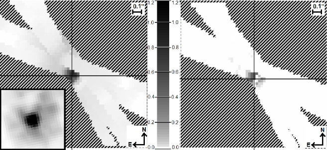
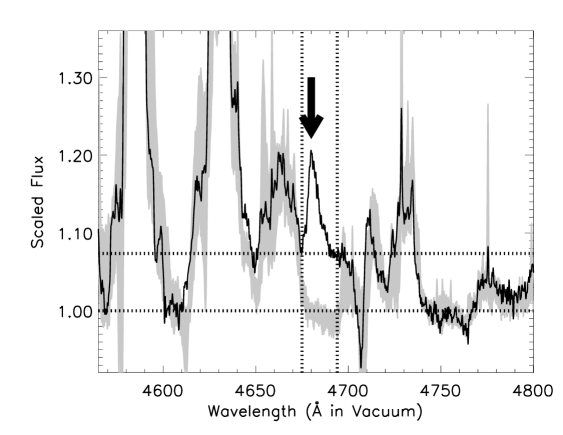
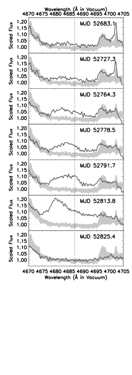
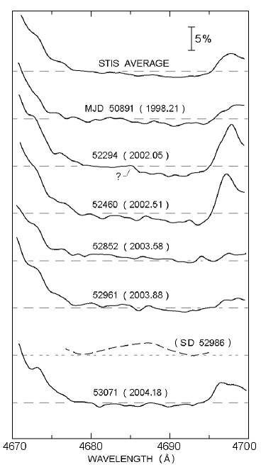
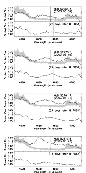
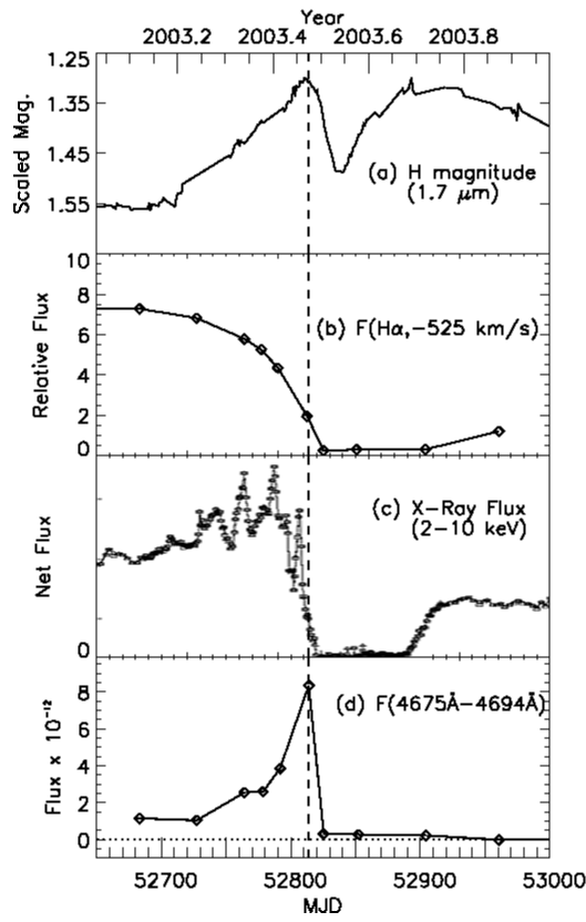
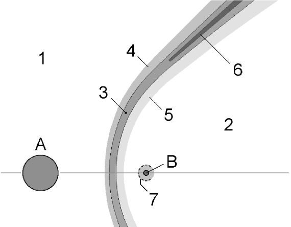
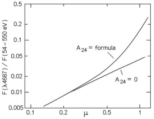
Wavelength	Relative	Predicted	Detection
(Å in Vacuum)	Strength	Flux	Limit	Notes
1640	8.150	601.	5.70	High extinction
2386	0.104	10.3	6.52	High extinction
2512	0.193	14.2	5.81	High extinction
2734	0.257	19.0	5.87	High extinction
3204	0.469	34.6	6.02	Confusion with other features
3797	0.003	0.221	9.26	Blend with Balmer line
3925	0.008	0.590	6.96
4101	0.015	1.11	8.75	Blend with Balmer line
4339	0.026	1.92	6.90	Blend with Balmer line
4543	0.036	2.66	7.18
4687	1.000	73.8	7.69
4861	0.053	3.91	7.82	Blend with Balmer H$\beta$
5413	0.080	5.90	16.0
6562	0.134	9.88	15.7	Blend with Balmer H$\alpha$
10126	0.237	17.5	19.8	High CCD noise

Table 2: Measured Flux and Equivalent Width of the 4680Å Feature

		Continuum		Line	Line EW
MJD	Year	Level	$S/N$	Flux	(Å)
50891.4	1998.21	1.32	79	-0.12$\pm$0.22	-0.09$\pm$0.16
51230.5	1999.14	2.27	126	-0.47$\pm$0.23	-0.21$\pm$0.10
51623.8	2000.22	3.16	140	-0.10$\pm$0.30	-0.03$\pm$0.09
52016.8	2001.29	2.71	109	-0.63$\pm$0.32	-0.23$\pm$0.12
52294.0	2002.05	2.65	110	-0.26$\pm$0.31	-0.10$\pm$0.12
52459.5	2002.51	2.58	130	-0.29$\pm$0.26	-0.11$\pm$0.10
52683.1	2003.12	2.49	121	0.82$\pm$0.27	0.33$\pm$0.11
52727.3	2003.24	2.65	102	0.67$\pm$0.34	0.25$\pm$0.13
52764.3	2003.34	2.36	97	2.20$\pm$0.32	0.93$\pm$0.13
52778.5	2003.38	2.56	118	2.22$\pm$0.28	0.87$\pm$0.11
52791.7	2003.42	2.74	144	3.35$\pm$0.25	1.23$\pm$0.09
52813.8	2003.47	3.09	107	7.38$\pm$0.37	2.38$\pm$0.12
52825.4	2003.51	3.18	113	0.25$\pm$0.37	0.08$\pm$0.11
52852.4	2003.58	3.25	108	0.06$\pm$0.39	0.02$\pm$0.12
52904.3	2003.72	4.38	148	-0.03$\pm$0.34	-0.01$\pm$0.09
52960.6	2003.88	4.80	150	-0.03$\pm$0.37	-0.01$\pm$0.09
53071.2	2004.18	4.69	140	-0.28$\pm$0.44	-0.06$\pm$0.09

Table 3: Relative Noise Levels and Constraints on He II Emission in STIS Data Before 2003.00 and After 2003.50

MJD	Year	$S/N$	E.W. (mÅ)
50891	1998.21	127	+24$\pm$36
51230	1999.14	133	+1$\pm$34
51624	2000.22	109	-50$\pm$42
52017	2001.29	114	-61$\pm$40
52294	2002.05	137	+14$\pm$34
52460	2002.51	119	+33$\pm$38
52683	2003.12	102	+182$\pm$45
52825	2003.51	137	-37$\pm$36
52852	2003.58	164	+44$\pm$29
52904	2003.72	128	+27$\pm$36
52961	2003.88	130	+43$\pm$35
53071	2004.18	156	+18$\pm$29
(avg)	$\cdots$	345	-11$\pm$14

References

- Cardelli et al. (1989) Cardelli, J. A., Clayton, G. C., & Mathis, J. S. 1989, ApJ, 345, 245
- Corcoran et al. (2001) Corcoran, M. F., et al. 2001, ApJ, 562, 1031
- Corcoran et al. (2004) Corcoran, M. F., et al. 2004, ApJ, 613, 381
- Corcoran (2005) Corcoran, M. F. 2005, AJ, 129, 2018
- Cox et al. (1995) Cox, P., et al. 1995, A&A, 297, 168
- de Vaucouleurs & Eggen (1952) de Vaucouleurs, G. & Eggen, O. J. 1952, PASP, 64, 185
- Damineli (1996) Damineli, A. 1996, ApJ, 460, L49
- Davidson & Netzer (1979) Davidson, K., & Netzer, H. 1979, Revs. Mod. Phys. 51, 715
- Davidson & Humphreys (1997) Davidson, K. & Humphreys, R. M. 1997, ARA&A, 35, 1
- Davidson et al. (1995) Davidson, K., et al. 1995, AJ, 109, 1784
- Davidson (1999) Davidson, K. 1999, Astronomical Society of the Pacific Conference Series, 179, 304
- Davidson et al. (2000) Davidson, K., Ishibashi, K., Gull, T. R., Humphreys, R. M., & Smith, N. 2000, ApJ, 530, L107
- Davidson et al. (2001) Davidson, K., Smith, N., Gull, T. R., Ishibashi, K., & Hillier, D. J. 2001, AJ, 121,1569
- Davidson (2002) Davidson, K. 2002, Astronomical Society of the Pacific Conference Series, 262, 267
- Davidson (2004a) Davidson, K. 2004a, STScI Newsletter, Spring 2004, 1
- Davidson et al. (2005a) Davidson, K., Martin, J. C., Humphreys, R. M., Ishibashi, K., Gull, T. R., Stahl, O., Weis, K., Hiller, D. J., Damineli, A., Corcoran, M., & Hamann, F. 2005a, AJ, 129, 900
- Davidson (2005b) Davidson, K. 2005b, Astronomical Society of the Pacific Conference Series, 332, 103
- Fitzpatrick (1999) Fitzpatrick, E. L. 1999, PASP, 111, 63
- Feast et al. (2001) Feast, M., Whitelock, P., & Marang, F. 2001, MNRAS, 322, 741
- Gaviola (1953) Gaviola, E. 1953, ApJ, 118, 234
- Gull (2005) Gull, T. 2005, Astronomical Society of the Pacific Conference Series, 332, 281
- Hamaguchi et al. (2004) Hamaguchi, K., Corcoran, M. F., Gull, T., White, N. E., Damineli, A., & Davidson, K. 2004, ArXiv Astrophysics e-prints, astro-ph/0411271, to appear in “Massive Stars in Interacting Binaries” held in Quebec Canada (16-20 Aug, 2004)
- Hillier et al. (2001) Hillier, D. J., Davidson, K., Ishibashi, K., & Gull, T. 2001, ApJ, 553, 837
- Hillier et al. (2005) Hillier, D. et al. 2005, in preparation
- Humphreys & Koppelman (2005) Humphreys, R. M., & Koppelman, M. 2005, Astronomical Society of the Pacific Conference Series, 332, 161
- Ishibashi et al. (1999) Ishibashi, K., Corcoran, M. F., Davidson, D., Swank, J. H., Peetre, R., Drake, S. A., Damineli, A., & White, S. 1999, ApJ, 525, 983
- Ishibashi (2001) Ishibashi, K. 2001, ASP Conf. Ser. 242: Eta Carinae and Other Mysterious Stars: The Hidden Opportunities of Emission Spectroscopy, 242, 53
- Johnson (1968) Johnson, H. M. 1968, in Stars and Stellar Systems, Chicago: University of Chicago Press, 1968, edited by Middlehurst, Barbara M.; Aller, Lawrence H., 65
- Lamers & Cassinelli (1999) Lamers, H. J. G. L. M., & Cassinelli, J. P. 1999, Introduction to Stellar Winds / Henny J.G.L.M. Lamers and Joseph P. Cassinelli. Cambridge ; New York : Cambridge University Press, 1999. ISBN 0521593980, p.211
- McKenna et al. (1997) McKenna, F. C., Keenan, F. P., Hambly, N. C., Allende Prieto, C., Rolleston, W. R. J., Aller, L. H., & Feibelman, W. A. 1997, ApJS, 109, 225
- Martin (2005) Martin, J.C. 2005, Astronomical Society of the Pacific Conference Series, 332, 114
- Meaburn et al. (1987) Meaburn, J., Wolstencroft, R. D., & Walsh, J. R. 1987, A&A, 181, 333
- Morrison & McCammon (1983) Morrison, R., & McCammon, D. 1983, ApJ, 270, 119
- O’Connell (1956) O’Connell, D. J. K. 1956, Vistas in Astronomy, 2, 1165
- Osterbrock (1989) Osterbrock, D. E. 1989, Astrophysics of Gaseous Nebulae and Active Galactic Nuclei, (Mill Valley, CA: University Science Books)
- Pittard et al. (1998) Pittard, J. M., Stevens, I. R., Corcoran, M. F., & Ishibashi, K. 1998, MNRAS, 299, L5
- Pittard & Corcoran (2002) Pittard, J. M. & Corcoran, M. F. 2002, A&A, 383, 636
- Smith et al. (2003) Smith, N., Davidson, K., Gull, T. R., Ishibashi, K., & Hillier, D. J. 2003, ApJ, 586, 432
- Stahl et al. (2005) Stahl, O., Weis, K., Bohmans, D. J., Davidson, K., Gull, T. R., & Humphreys, R. M. 2005, A&A, in press.
- Steiner & Damineli (2004) Steiner, J. E., & Damineli, A. 2004, ApJ, 612, L133
- Stevens et al. (1992) Stevens, I. R., Blondin, J. M., & Pollock, A. M. T. 1992, ApJ, 386, 265
- Thackeray (1953) Thackeray, A. D. 1953, MNRAS, 113, 211
- Viotti et al. (2002) Viotti, R. F., et al. 2002, A&A, 385, 874
- Whitelock et al. (1994) Whitelock, P. A., Feast, M. W., Koen, C., Roberts, G., & Carter, B. S. 1994, MNRAS, 270, 364
- Whitelock et al. (2004) Whitelock, P. A., Feast, M. W., Marang, F., & Breedt, E. 2004, MNRAS, 352, 447
- Zanella et al. (1984) Zanella, R., Wolf, B., & Stahl, O. 1984, A&A, 137, 79
- Zethson (2001) Zethson, T. 2001, Ph.D. Thesis, Lunds Universitet