Towards a physical model of dust tori in Active Galactic Nuclei

We explore physically self-consistent models of dusty molecular tori in Active Galactic Nuclei (AGN) with the goal of interpreting VLTI observations and fitting high resolution mid-IR spectral energy distributions (SEDs). The input dust distribution is analytically calculated by assuming hydrostatic equilibrium between pressure forces – due to the turbulent motion of the gas clouds – and gravitational and centrifugal forces as a result of the contribution of the nuclear stellar distribution and the central black hole. For a fully three-dimensional treatment of the radiative transfer problem through the tori we employ the Monte Carlo code MC3D. We find that in homogeneous dust distributions the observed mid-infrared emission is dominated by the inner funnel of the torus, even when observing along the equatorial plane. Therefore, the stratification of the distribution of dust grains – both in terms of size and composition – cannot be neglected. In the current study we only include the effect of different sublimation radii which significantly alters the SED in comparison to models that assume an average dust grain property with a common sublimation radius, and suppresses the silicate emission feature at $9.7\,\muup$m. In this way we are able to fit the mean SED of both type I and type II AGN very well. Our fit of special objects for which high angular resolution observations ($\leq$ 0.3″) are available indicates that the hottest dust in NGC 1068 reaches the sublimation temperature while the maximum dust temperature in the low-luminosity AGN Circinus falls short of 1000 K.

1 Introduction

Active galaxies are among the most energetic objects in the universe. With current knowledge, these objects – although containing up to 60 different variations (Ward 2003) – can be described by a small number of models. The differences between them can be reduced to geometrical effects. The most common model is called the Unified Scheme (Antonucci 1993) of Active Galactic Nuclei (AGN). According to this scheme, several components can be distinguished: A supermassive black hole ($10^{6}$ - $10^{10}\,M_{\sun}$) in the centre surrounded by an accretion disc, reaching from the marginally stable orbit up to several thousands of Schwarzschild radii. By turbulent processes, material is accreted and the gas in the disc is heated to several hundred thousand Kelvin. Hence, the spectrum of the emitted radiation peaks in the UV/optical wavelength range. In the outer part, the temperature of the disc drops to about 1000 K, at the start of the larger and geometrically thicker dust reservoir, producing a characteristic bump in the IR spectral range (hereafter the IR bump).

The Unified Scheme differentiates between two different types of active galaxies: The spectral energy distributions (SEDs) of type I objects show the so-called blue bump, arising from the direct radiation of the accretion disc mentioned above. Broad emission lines overlay the continuum spectral energy distribution. They come from the so-called Broad Line Region (BLR) near the centre of the object. Within this area, gas clouds are moving at high velocities due to the deep potential well of the central black hole and, therefore, emit broad spectral lines. Type II objects do not show a big blue bump and are characterised by narrow spectral lines, arising from orbiting gas clouds further away from the gravitational centre. After broad spectral lines were observed in the polarised light of a type II object, it was proposed that both AGN types belong to the same class of object with a dust reservoir located in a torus which blocks the direct view to the centre and the BLR within the opening of the torus for the case of type II objects. Polarised light is then produced by electrons and material above the opening angle of the dust torus. Therefore, the type of object simply depends on the viewing angle towards the torus.

More direct evidence for the existence of an obscuring torus comes from recent observations of the prototype Seyfert II galaxy NGC 1068 in the mid-infrared by the VLTI with MIDI (Leinert et al. 2003). Based on these interferometric data, Jaffe et al. (2004) distinguished two different dust components: a hot component in the centre with a diameter of less than 1 pc and a temperature of more than 800 K and warm dust within an elongated structure perpendicular to the jet axis with a temperature of approximately 320 K and a size of 3.4 pc times 2.1 pc perpendicular and parallel to the torus axis, respectively. This means that geometrically thick tori are consistent with the data.

The first more detailed radiative transfer simulations for the case of dusty tori were carried out by Pier & Krolik (1992). They used the most simple dust configuration to describe the observations available at that time, consisting only of spectral energy distributions – due to the large distances (several tens of Mpc) and small sizes (less than 100 pc) of these objects: a cylindrical shape with a cylindrical hole in the middle. Although pointing out that dust – in order to avoid destruction by hot gas – must be contained in clumps, they applied a homogeneous dust distribution. Characteristics of their modelling are the small sizes of a few pc in diameter and very high dust densities. The small amount of cold dust leads to a too narrow dust temperature range, resulting in spectra insufficiently extended towards longer wavelengths, compared to observations. Granato & Danese (1994) preferred larger wedges (tens to hundreds of pc in diameter) and thereby solved the problem of the too narrow IR bumps compared to observations. Further difficulties when comparing calculations with data emerge from the so-called silicate feature problem. The silicate feature is a resonance in the spectral energy distributions at $9.7\,\muup$m, arising from the stretching modes in silicate tetrahedra. For optically thin configurations, this feature is seen in emission. Looking at optically thick tori, two cases have to be distinguished: The feature appears in emission, if the temperature decreases along the line of sight away from the observer and an absorption feature is seen for the case of increasing temperature along the line of sight. Between those two cases, at an optical depth $\tau_{9.7\,\muup\mathrm{m}}\,\approx\,1$, a mixture of both – so-called self-absorption – is visible (Henning 1983). Therefore, for typical torus geometries, the feature is expected to arise in absorption for type II objects and in emission in type I sources. Up to now, no observation of a type I object has shown the feature in emission. In both studies mentioned, a significant reduction of the silicate emission-feature could be found for the case of type I galaxies. However, a lot of fine tuning of the parameters was needed. Granato & Danese (1994) point out that small silicate grains are selectively destroyed by radiation pressure induced shocks in the inner part of the torus close to the central source. Therefore, they set up a depletion radius for small silicate grains and are able to reduce the silicate emission at $9.7\muup$m. Manske et al. (1998) succeeded in avoiding the feature by using a toroidal density distribution comparable to the one of Granato & Danese (1994) with a large optical depth in combination with a strong anisotropic radiation source, which is a more physical approach to describe the accretion disc. Another more realistic way to cope with the silicate feature problem was proposed by Nenkova et al. (2002). They introduce a clumpy structure again within a flared disc geometry. Their radiative transfer simulations show that within a large range of values of their parameters, a reduction of the emission feature is feasible. Another possibility to investigate AGN torus models is the simulation of polarisation maps and their comparison with observations. For a first approach see Wolf & Henning (1999).

In this first paper of a series, we present radiative transfer calculations for a hydrostatic model of dusty tori. We use the so-called Turbulent Torus Model, introduced by Camenzind (1995). The great advantage of this model arises from the fact that the dust density distribution and the geometrical shape of the torus do not have to be set up arbitrarily and independent of each other, but both result from physically reasonable assumptions. Our calculations combine structure modelling and fully three-dimensional Monte Carlo radiative transfer simulations. The following chapter will summarise the structure modelling together with all ingredients needed to perform the radiative transfer simulations.

In a further step towards more physical models of AGN dust tori, the homogeneous dust distribution will be replaced by a clumpy dust model. Later, we will start with hydrodynamic simulations in combination with radiative transfer calculations, in order to gain information about the temporal evolution of spectral energy distributions and surface brightness maps of dusty tori.

Chapter 3 deals with the results we obtained with the first approach. Spectral energy distributions and surface brightness maps are calculated and discussed for part of the simulation series we conducted. In chapter 4 we discuss comparisons of our model results with large aperture data as well as with very high spatial resolution data.

2 The model

2.1 The Turbulent Torus Model

It is known that many spiral galaxies harbor young nuclear star clusters (e.g. Gallimore & Matthews 2003; Walcher et al. 2004; Böker et al. 2002, 2004). Especially during late stages of stellar evolution, stars release large amounts of gas through stellar winds and the ejection of planetary nebulae. With increasing distance from the star, dust forms from the gas phase. Due to the origin of the dust from ejection processes of single stars, we expect the dust torus to consist of a cloudy structure. As even current interferometric instruments are not able to resolve single clouds of the dust distribution, they are assumed to be small. For the sake of simplicity, we treat the torus as a continuous medium in this paper. The dust clouds are ejected by the stars and therefore take over the stellar velocity dispersion $\sigma_{*}$. As we neglect interaction effects between these clouds, we can assume that they possess the same velocity as the stars, called the turbulent velocity $v_{\mathrm{t}}$ ($v_{\mathrm{t}}\approx\sigma_{*}$).

We are dealing with stationary models only. Therefore, the presence of continuous energy feedback by supernovae explosions as well as continuously injected mass by stellar winds is not taken into account. The dust clouds are embedded into hot gas, which leads to the destruction of dust grains by sputtering effects. Therefore, dust has a finite lifetime and it is likely that the composition differs from the one found in interstellar dust within our galaxy (see Sect. 2.3). The effects of magnetic fields on charged dust particles are neglected. The radiation pressure of the extreme radiation field of the central AGN exerted on the dust grains only affects the very innermost part of the dust density distribution and is therefore not taken into account within our simulations.

Due to their environment, the dusty clouds are subject to gravitational forces. Together with centrifugal forces – because of the rotation of the central star cluster – an effective potential can be formed. In the following, the three main components will be discussed: First, the gravitational potential of the supermassive black hole. As the torus extends to several hundred thousands of Schwarzschild radii from the centre, we can treat the black hole as a point-like source of gravitation with a Newtonian potential, given in cylindrical coordinates:

$$\phi_{\mathrm{BH}}(R,z)=-\frac{G\,M_{\mathrm{BH}}}{\sqrt{R^{2}+z^{2}}}.$$ (1)

The second contribution we take into account is the gravitational potential of the nuclear star cluster, dominating the contribution by stars in the galaxy core. From high resolution observations of the centres of galactic nuclei (e. g.  Gebhardt et al. 1996) a surface brightness distribution profile can be derived. This can be well fitted by a two-component power law, the so-called Nuker law, given by the following equation (Lauer et al. 1995; Byun et al. 1996; Gebhardt et al. 1996; Faber et al. 1997a):

$$I(R,z) = 2^{\frac{\beta-\delta}{\alpha}}\,I_{\mathrm{c}}\,\left(\frac{R_{\mathrm{c}}}{\sqrt{R^{2}+z^{2}}}\right)^{\delta}$$ (2)

$$\left[1+\left(\frac{\sqrt{R^{2}+z^{2}}}{R_{\mathrm{c}}}\right)^{\alpha}\right]^{\frac{\delta-\beta}{\alpha}},$$

where $R_{\mathrm{c}}$ is the core radius (or break radius), $\beta$ the slope of the surface brightness distribution outside $R_{\mathrm{c}}$, $\delta$ the slope inside $R_{\mathrm{c}}$, $\alpha$ characterises the width of the transition region and $I_{\mathrm{c}}$ is the surface brightness at the location of $R_{\mathrm{c}}$.

When assuming a constant mass-to-light ratio, this distribution mirrors the projected mass density distribution directly. By applying a least-square fitting procedure, one can obtain the 3D density profile, for which an analytical expression can be given. This is the so-called Zhao density profile family (Zhao 1997):

$$\rho_{*}(R,z)=\frac{M_{*}}{4\,\pi\,R_{\mathrm{c}}^{3}}\,\frac{C\left(\tilde{\alpha},\tilde{\beta},\tilde{\delta}\right)}{\left(R^{2}+z^{2}\right)^{\frac{\tilde{\delta}}{2}}\,\left(1+\left(R^{2}+z^{2}\right)^{\frac{\tilde{\alpha}}{2}}\right)^{\frac{\tilde{\beta}-\tilde{\delta}}{\tilde{\alpha}}}},$$ (3)

where the parameters $\tilde{\alpha}$, $\tilde{\beta}$ and $\tilde{\gamma}$ are complicated functions of the parameters $\alpha$, $\beta$ and $\gamma$ of the Nuker law. The quantity $C$ is a constant, depending on these parameters.

By solving the Poisson equation, the gravitational potential of the nuclear star cluster can be obtained. Throughout this paper, all simulations use the special case of the Hernquist profile (Hernquist 1990). According to observed profiles of cores of spiral galaxies, the exponent of the density distribution within the core radius is close to 1 in most cases (corresponding to the Hernquist profile). Recent simulations of dark matter halos by Williams et al. (2004) – which belong to the same family of stellar systems – also give an upper limit for the exponent of the density distribution within the core radius between 1.5 and 1.7 in the inner part.
With the parameters $\tilde{\alpha}$ = $1$, $\tilde{\beta}$ = $4$ und $\tilde{\delta}$ = $1$, we finally get the needed gravitational potential:

$$\phi_{\mathrm{Hernquist}}(R,z)=-\frac{G\,M_{*}}{\sqrt{R^{2}+z^{2}}+R_{\mathrm{c}}}.$$ (4)

The third part of the effective potential is the centrifugal potential. Apart from the turbulent velocity, the stars – and therefore the dust clouds – possess an additional velocity component from the rotational motion around the gravitational centre. Due to the lack of observational data, we adopt the following distribution of specific angular momentum for such a stellar system:

$$j_{\mathrm{spec}}=\sqrt{G\,(M_{\mathrm{BH}}\,+M_{*}(R_{\mathrm{T}}))\,R_{\mathrm{T}}}\,\left(\frac{R}{R_{\mathrm{T}}}\right)^{\gamma}.$$ (5)

Here, $R_{\mathrm{T}}$ is the torus radius, defined as the location, where the effective potential reaches its minimal value. This corresponds to an equilibrium of centrifugal and gravitational forces in our solution, where the angular momentum attains the Keplerian value. Therefore, a distribution of the specific angular momentum is needed, which fixes the value at the location of the torus radius to the Keplerian value. We used a less steep decline of the specific angular momentum beyond the torus radius than for the Keplerian case, which is in agreement with expectations for elliptical star clusters. Such toroidal gas distributions are expected to be unstable on time scales larger than the dynamical time at the torus radius. The torus is however steadily refilled so that a quasi-stationary configuration results.

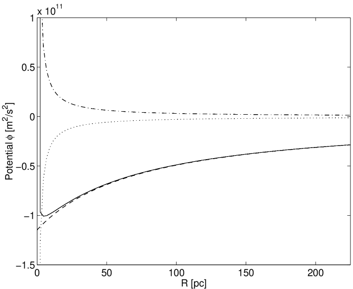
Figure 1: Comparison of the contributions of the three components of the effective potential for the parameters of our standard model in the equatorial plane. The solid line corresponds to the effective potential, the dotted line to the BH-potential, the dashed line to the potential of the nuclear star cluster and the dashed-dotted line to the centrifugal potential.

By integrating over the centrifugal force – under the assumption of constant angular velocity on cylinders – we obtain the centrifugal potential:

$$\phi_{\mathrm{CF}}(R,z)=\frac{G\,(M_{\mathrm{BH}}\,+M_{*}(R_{\mathrm{T}}))}{2\,R_{\mathrm{T}}\,(1-\gamma)}\,\left(\frac{R}{R_{\mathrm{T}}}\right)^{2\,(\gamma-1)}.$$ (6)

The effective potential and its three single components are shown in Fig. 1 for the case of our standard model (described in Sect. 2.2) in the equatorial plane. As can be seen, the effective potential (given by the solid line) in the outer part of the torus is dominated by the potential of the nuclear star cluster (dashed line). Moving closer to the centre, the black hole potential (dotted line) wins, which leads to a further bending down of the potential, before the centrifugal potential (dashed-dotted line) dominates. The latter is the only repulsive term and leads to a centrifugal barrier close to the centre, preventing the models to be gravitationally unstable.

The force given by the effective potential has to be balanced by the turbulent pressure in hydrostatic equilibrium. This pressure results from the turbulent motion of the dust clouds and can be expressed by the following (isothermal) equation of state:

$$P(\rho_{\mathrm{d}})=\rho_{\mathrm{d}}\,v_{\mathrm{t}}^{2}.$$ (7)

After inserting this into the equation for the hydrostatic equilibrium and solving the differential equation under the assumption that $v_{\mathrm{t}}$ is constant, we obtain the dust density distribution:

$$\rho_{\mathrm{d}}=\rho_{\mathrm{d}}^{0}\,\exp\left[\frac{G\,M_{*}}{v_{\mathrm{t}}^{2}\,R_{\mathrm{c}}}\,\left\{\frac{M_{\mathrm{BH}}/{M_{*}}}{\sqrt{\frac{R^{2}+z^{2}}{R_{\mathrm{c}}^{2}}}}+\frac{1}{1+\sqrt{\frac{R^{2}+z^{2}}{R_{\mathrm{c}}^{2}}}}\right.\right.$$

$$\left.\left.{}-\frac{R_{\mathrm{c}}\,(M_{\mathrm{BH}}\,+M_{*}(R_{\mathrm{T}}))}{2\,M_{*}\,R_{\mathrm{T}}(1-\gamma)}\,\left(\frac{R}{R_{\mathrm{T}}}\right)^{2\,(\gamma-1)}\right\}\right].$$ (8)

Here, $\rho_{\mathrm{d}}^{0}$ is a measure for the total dust mass. From this equation, some basic features of the model can be derived: First of all, equipotential surfaces have the same shape as surfaces of constant density, so-called isopynic surfaces. The shape of these surfaces only depends on the reduced parameter $M_{\mathrm{BH}}/{M_{*}}$ and the reduced coordinates $R/{R_{\mathrm{c}}}$, $R/{R_{\mathrm{T}}}$ and $z/{R_{\mathrm{c}}}$ and the exponent of the angular momentum distribution $\gamma$. As mentioned above, the torus radius is connected with the minimum of the potential, the maximum of the density and the maximum of pressure and lies within the equatorial plane, due to symmetry considerations.

2.2 Parameters of the model

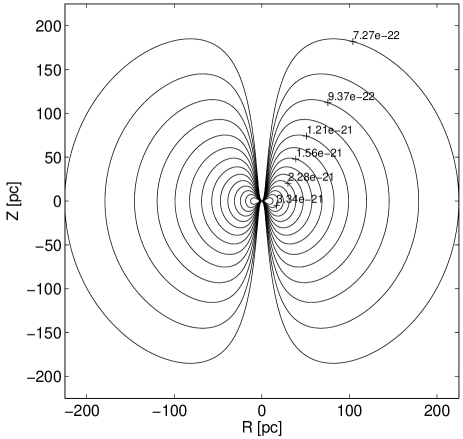
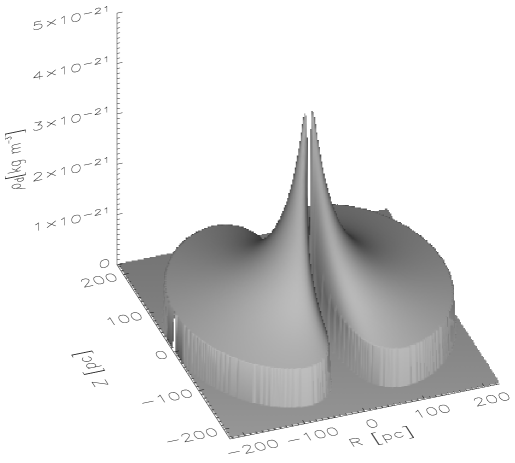
Figure 2: Visualisation of our standard model: a) Isopynic line plot (logarithmically equidistant) in a meridional plane of the torus. The numbers give the dust density in kg $\mathrm{m}^{-3}$ of the corresponding isopynic line. b) Dust density distribution in a meridional plane.

The introduced standard model will be used to represent the core of a typical Seyfert galaxy. Therefore, we calculated the mean black hole mass and mean luminosity of a large sample of Seyfert galaxies, given in Woo & Urry (2002). We find mean values of $\left<M_{\mathrm{BH}}\right>$ =  $6.6\cdot 10^{7}\,\mathrm{M}_{\odot}$ and $\left<L_{\mathrm{disc}}\right>$ = $1.2\cdot 10^{11}\,\mathrm{L}_{\odot}$. After calculating a set of simulations with different dust density distributions, leading to different density contrasts between the maximum density and the outer part of the distribution, we found that a relatively shallow density distribution is needed in order to obtain SEDs extending to wavelengths longer than 10-20$\,\muup$m. To achieve this, a relatively steep radial distribution of specific angular momentum is required ($\gamma$ = $0.5$ leads to the steepest – but still stable – distribution). But this gives only a fairly small effect. It is more efficient to increase the core radius, which leads to a broadening of the density distribution, due to the flattening of the potential of the star cluster in the outer part of the torus. A change of the total mass of the stars mainly scales the potential of the stellar cluster and therefore finally the density distribution. By taking this into account, we chose the core radius for our mean model to be $75\,$pc with a mass of the nuclear star cluster of $2\cdot 10^{9}\,\mathrm{M}_{\odot}$.

To constrain the other parameters, one can use the fact that not all of them are independent from each other. Comparable to the fundamental plane of global galaxy parameters, the cores of ellipticals and bulges of spiral galaxies span the so-called core fundamental plane, relating the parameters core radius $R_{c}$, the central surface brightness $\mu_{0}$ and the central velocity dispersion $\sigma_{*}$ (Kormendy 1987; Faber et al. 1997b). These studies give several relations between relevant parameters. The relation between the core radius and the central velocity dispersion of the stars is interesting for us:

$$\sigma_{*}\approx 201\,\left(\frac{R_{\mathrm{c}}}{75\,\mathrm{pc}}\right)^{0.18}\,\frac{\mathrm{km}}{\mathrm{s}}.$$ (9)

Table 1: Parameters used for the simulation of our mean Seyfert model.

Parameter	Value
$M_{\mathrm{BH}}$	$6.64\cdot 10^{7}\,M_{\sun}$
$R_{\mathrm{c}}$	75 pc
$M_{*}$	$2.0\cdot 10^{9}\,M_{\sun}$
$L_{\mathrm{disc}}$	$1.23\cdot 10^{11}\,L_{\sun}$
$L_{\mathrm{disc}}/{L_{\mathrm{Edd}}}$	6%
$R_{\mathrm{T}}$	5 pc
$M_{\mathrm{dust}}$	$5.79\cdot 10^{5}\,M_{\sun}$
$\tau_{9.7\,\muup\mathrm{m}}$	2.0
$R_{\mathrm{out}}$	225 pc
$v_{\mathrm{t}}$	$201\,\mathrm{km}\,\mathrm{s}^{-1}$
$\gamma$	0.5
$d$	45 Mpc

As already mentioned above, the dusty clouds are produced by the stars and take over their velocity dispersion. Therefore, we choose the turbulent velocity of the clouds $v_{\mathrm{t}}$ to be equal to the velocity dispersion of the stars in the central region of the galaxy. According to equation (9) the value $v_{\mathrm{t}}$ = $201\,\mathrm{km}\,\mathrm{s}^{-1}$ is obtained. Interactions between the different phases (dust, molecular and hot gas) within the torus and between other dust clouds, which may alter their velocity distribution are not taken into account at present. The outer radius of the torus is chosen to be three times the core radius of the nuclear star cluster, where the density distribution has already reached an approximately constant value. An upper limit for the total mass of the nuclear star cluster is determined by the Jeans equation, which relates structural with dynamical parameters for an isothermal model of the central stellar distribution under the assumption of a constant velocity dispersion. The remaining two parameters $R_{\mathrm{T}}$ and $\gamma$ are chosen such that the dust density distribution remains flat enough to obtain IR bumps, which are broad enough to compare with data and to obtain a torus model with an inner radius small enough to allow the majority of the grain species to reach their sublimation temperatures. Finally, the mass of the dust, enclosed into the torus, is determined by the depth of the silicate feature at $9.7\,\muup$m. We chose $M_{\mathrm{dust}}$ = $5.79\cdot 10^{5}\,M_{\sun}$ (corresponding to an optical depth of $\tau_{9.7\,\muup\mathrm{m}}$ = $2.0$), which yields depths comparable to observed spectra.

The parameters we assumed for our standard model are summarised in Table 1 and the resulting model is shown in Fig. 2. As can be seen, the torus has a relatively dense core and the density distribution gets shallow in the outer part. The maximum is reached in the equatorial plane (due to symmetry considerations) at the torus radius $R_{\mathrm{T}}$ and the models possess a more or less pronounced cusp at the inner end of the torus. The dust-free cone with quite steep walls will be called funnel in the following. The turbulent velocity always tends to increase the height of the torus, while the angular momentum tends to flatten it.

2.3 Dust properties

Although the very extreme physical conditions near the central source make it likely that the dust composition may be altered compared to interstellar dust in our own galaxy, we assume – for the sake of simplicity and comparability – a typical dust extinction curve of interstellar dust. We use the model of Mathis et al. (1977) which fits well the observed extinction curve of the interstellar medium.

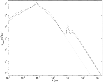
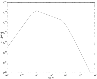
Figure 3: Input parameters of our simulations: a) Course of the mass extinction coefficient plotted against the wavelength for the averaged dust model (dashed line) and single grains (solid line): composition of silicate and graphite grains with varying grain radii (for details see text). The dotted straight line should clarify the offset in the continuum extinction curve. b) SED of the central accretion disc, used as the primary energy source.

They found a number density distribution (MRN-distribution hereafter), which is proportional to the grain radius to the power of - 3.5 and a range of grain radii between $0.005\,\muup$m and $0.25\,\muup$m. We use 15 different grains, containing a mixture of 5 silicate and 10 graphite grains – each species with different grain radii according to the MRN grain size distribution – and a mass fraction of 62.5% silicate and 37.5% graphite. Because of the anisotropic behaviour of graphite, two different sets of optical constants are necessary: one where the electric field vector oscillates parallel to the crystal axis of the grain (5 grains) and another one, where it oscillates perpendicular to it (5 grains). For them, the standard $\frac{1}{3}\,-\,\frac{2}{3}$ approximation is used, which is valid exactly in the Rayleigh limit and reproduces extinction curves reasonably well, as shown by Draine & Malhotra (1993). Optical data (refraction indices) are taken from Draine & Lee (1984), Laor & Draine (1993) and Weingartner & Draine (2001) and the scattering matrix elements and coefficients are calculated under the assumption of spherical grains using the routines of Bohren & Huffman (1983) within the radiative transfer code MC3D, which will be discussed in Sect. 2.5.

In addition, a comparison was made between a split into 15 different grains and the usage of only one grain, but with weighted mean values for the extinction, absorption and scattering cross sections and the Stokes parameters, which describe the intensity and the polarisation state of the photon package. The weights result from the abundance and the size distribution of the respective material (for details about the averaging see Wolf (2003a)). The resulting extinction curves of these two cases are shown in Fig. 3a, where the solid line corresponds to the splitted model and the dashed line to the model with mean characteristics. For every dust species (type of material and grain size) the temperature distribution is determined separately. In Fig. 3a one can clearly see the two silicate features at $9.7\,\muup\mathrm{m}$ and $18.5\,\muup\mathrm{m}$. The extinction curves drop down quite steeply at longer wavelengths and an offset can be recognised around the wavelengths of the two features between the continuum spectra shortward of $10\,\muup$m and longward of $20\,\muup$m, emphasised by the dotted line fragment.

2.4 Primary source

In our modelling, the dust in the torus is solely heated by an accretion disc in the centre of the model space. In most of the simulations we use a point-like, isotropically radiating source with a luminosity of $1.2\cdot 10^{11}\,\mathrm{L}_{\odot}$ in our standard model, which corresponds to roughly $6\%$ of the Eddington luminosity. The spectral energy distribution (SED) is composed of different power laws and a Planck curve as follows. In the ultraviolet to optical wavelength regime, we use the composite mean quasar spectrum from Manners (2002). For wavelengths longer than Lyman alpha, it includes data from 2200 quasars of the Sloan Digital Sky Survey (Vanden Berk et al. 2001), which results in a power law with a spectral index of $\alpha_{\nu}\,$=$\,-0.46$ . Shortwards of Lyman alpha, data from radio-quiet quasars (Zheng et al. 1997), taken with the HST Faint Object Spectrograph, is used. The data leads to a spectral index of $\alpha_{\nu}$ = $-1.8$. For wavelengths longer than $10\,\muup$m, we use a decline of the spectrum according to the Rayleigh-Jeans branch of a Planck curve with an effective temperature of 1000 K, reflecting the smallest temperatures expected from the thermal emission of the accretion disc. At shorter wavelengths, the spectrum decays with a spectral index of $\alpha_{\nu}$ = $-3$. Due to the lack of observational data in this wavelength range, the index is chosen in agreement with theoretical modelling of accretion disc spectra performed by Hubeny et al. (2000). Taking this shape and normalising to the chosen bolometric luminosity of the accretion disc yields the input spectrum shown in Fig. 3b.

2.5 The radiative transfer code MC3D

MC3D is a three-dimensional continuum radiative transfer code based on the Monte Carlo approach (Fischer et al. 1994; Wolf et al. 1999). It is able to manage arbitrary three-dimensional dust and electron configurations and different primary sources of radiation. Diverse shapes and species of dust grains can be implemented as well. Working in the particle picture, the bolometric luminosity of the central source is divided into photon packages, so-called weighted photons. They are fully described by their wavelength $\lambda$ and their Stokes vector, describing the intensity and the polarisation state of the particle. According to a provided radiation characteristic and spectral energy distribution of the source, such a weighted photon is emitted. Within the dust or electron configuration, absorption and scattering take place, where Thomson scattering, Rayleigh and Mie scattering is applied to the weighted photon. In a last step, these photons are detected after leaving the convex model space.

According to this procedure, temperature distributions as well as – in a second step – spectral energy distributions and surface brightness distributions can be calculated. Temperature distributions have to be calculated using real radiative transfer. In order to minimise CPU time and get smoother surface brightness distributions, a raytracer (also inherent in MC3D) can be used to obtain SEDs and maps.

Details about MC3D and the built-in features can be found in Wolf et al. (1999), Wolf & Henning (2000), Wolf (2001) and Wolf (2003b).

Pascucci et al. (2004) tested MC3D for 2D structures against various other continuum radiative transfer codes, where they found good agreement. We also performed a direct comparison for the special case of AGN dust tori with the simulations of Granato & Danese (1994), one of the standard torus models to compare to, calculated with his grid based code.

Figure 4: Comparison of MC3D (solid line) with the code of Granato & Danese (1994) (dashed line).

The results are displayed in Fig. 4, where the solid line corresponds to the calculation with MC3D and the dashed line to the original spectrum of Granato. The underlying model is a wedge geometry with dust of constant density. The ratio between outer and inner radius is set to 100 with a half opening angle of the dust-free cone of 40 °  and an optical depth of 0.3 at $9.7\,\muup\mathrm{m}$ (for details of the model setup see Granato & Danese (1994)). The original spectrum of Granato’s code is taken from the library of SEDs described in Galliano et al. (2003).

As can be seen in Fig. 4, good agreement between the two codes is found with deviations smaller than 30% within the relevant wavelength range. The reason for the remaining differences between the two SEDs is due to the fact that only standard calibrations of the code-parameters were used and no fine tuning was performed. Minor differences of the model setup are responsible for the remaining discrepancies among the SEDs.

3 Results and discussion

First, the use of single dust grains is motivated, before we introduce our model by presenting temperature distributions and an inclination study. After that, several parameters of our standard model have been varied and the resulting effects will be discussed.

If not noted otherwise, all of the SEDs shown are pure dust re-emission spectra. The direct radiation from the central source is always omitted, as we are only interested in the mid-infrared wavelength range, where the torus emission dominates the SED. Optical depths are given for lines of sight within the equatorial plane from the centre outwards.

3.1 Averaged dust mixture versus single grains

Figure 5: SEDs at inclination angles of 0 °  and 90 °  for the case of averaged dust properties (dotted line) and dust splitted in grains of different species and sizes (solid line). The horizontal line segments in the left panel indicate the offset of the continuum SEDs of the individual curves.

Detailed Monte Carlo simulations are always very time consuming. In order to reduce the CPU time, an averaged dust grain mixture (Wolf 2003a) is often considered instead of a real mixture of single grains. However, temperature distributions have to be computed for every single grain. Therefore, computation time strongly scales with the number of dust grains considered. As Wolf (2003a) showed for the case of protoplanetary discs and we also confirmed for AGN tori, an averaged dust model works perfectly well, if the inner radius of the disc/torus is larger than the sublimation radii of the grains (see discussion later). But for most of our models, this is not the case, as the inner radii of the tori are often determined by sublimation themselves. These sublimation radii follow an approximative formula for the local thermodynamic equilibrium. It only takes emission of the central source and extinction by dust species with smaller inner radii into account. Although the resulting maximal temperatures for the single grains differ by up to 10% relative to the assumed sublimation temperatures of silicate and graphite grains, this seems to be an adequate procedure, as sublimation temperatures are not very well known. With this new dust model, the situation looks much different, as shown in Fig. 5, although the overall shape of the extinction curve looks similar compared to the one of the averaged grain model (see Fig. 3a). The typical shape of the resulting SEDs will be described in more detail in Sect. 3.3. In the following, we address just the major differences between these two cases. The solid line corresponds to our standard model (see Fig. 5) with a dust mixture containing 15 different grains (3 different grain species – silicate and two orientations of graphite grains – with 5 varying grain radii each), while the dotted line is calculated for the same torus parameters, but the dust model is given by a single grain type with averaged properties concerning chemical composition and grain size. Using the averaged grain model, the silicate features are much more pronounced compared to the other case. The same happens with the offset in the SED shortwards of the $9.7\,\muup\mathrm{m}$ feature. The reason for this is the varying sublimation temperatures of the different dust species. Silicate grains sublimate at about 1000 K, while graphite grains sublimate around 1500 K. Smaller particles are heated more efficiently than larger grains. Therefore, smaller grains reach the sublimation temperature earlier and the inner radius of their density distribution must be larger than the one for the distribution of large grains. This effect leads to a layering of grain species and sizes, where silicate grains are further out (in the radial direction) than graphite grains and the distribution of smaller grains is shifted outwards compared to the distribution of larger grains. Neglecting this layering and using averaged properties within one grain leads to the effects shown in Fig. 5. The reason for these effects is that some of the dust species, represented by the grain, are heated to temperatures higher than their sublimation temperatures. This is an unphysically treatment of these components. Especially affected are the smallest silicate grains, which are the most abundant ones in our dust model. The effects are mainly more explicitly visible characteristics of the dust extinction curve properties of silicate grains – especially the offset in the continuum spectrum near the feature (demonstrated by the horizontal lines in Fig. 5) and the strength of the feature itself. Reaching only the permitted smaller temperatures, these effects are partially balanced by the contribution of the other grain types. Using the minimum of sublimation temperatures of the mean grain components leads to a Wien branch shifted to longer wavelengths.

Being mainly interested in the mid-infrared wavelength range, we decided to split the dust model in single grains for all of the models shown in this paper. All species obey the same density distribution, according to physical reasoning (see Sect. 2.1) and the mass fraction of the individual species, derived from the power law number density distribution.

The inner radius of the distribution of every dust species is calculated using the formula for the local energy equilibrium and taking extinction by all other dust species into account. Spheres with these radii around the central source are left vacant concerning these particular dust species. The rest of the calculated equipotential surfaces are filled with dust, according to the dust model used.

3.2 Temperature distribution

Figure 6: Temperature distributions of the smallest silicate grain component: a) Radial temperature distributions. The solid line corresponds to an equatorial line of sight, the dotted line to an inclination angle of $i=30\,\degr$ and the dashed line to $i=20\,\degr$. b) Temperature distributions in $\theta$-direction. The solid line corresponds to a radial distance to the centre of 2 pc, the dotted line to 5 pc and the dashed line to 20 pc.

Figure 7: Comparison of the temperature distributions of different dust species within the equatorial plane: a) Temperature distributions for different sized silicate grains: $a=0.005\,\muup$m (solid line), $a=0.013\,\muup$m (dotted line), $a=0.035\,\muup$m (dashed line), $a=0.094\,\muup$m (dashed-dotted line), $a=0.25\,\muup$m (dashed-dotted-dotted-dotted line). b) Temperature distributions for different dust species: the smallest silicate component (solid line), the smallest graphite component with E $\parallel$ c (dotted line) and the smallest graphite component with E $\perp$ c (dashed line).

Fig. 6 shows the temperature distribution of our standard Seyfert model for the smallest silicate grain component, which is also the most abundant one (see Sect. 2.3). In the left panel, radial temperature distributions for an equatorial line of sight (solid line), an inclination angle of $i\,=\,30\,\degr$ (dotted line) and $i\,=\,20\,\degr$ (dashed line) are plotted. With increasing inclination angle, the intersection of the respective line of sight with the torus moves to larger distances from the central source (compare to Fig. 8b). Therefore, the maxima of the temperature distributions move further out and the maximum temperature decreases as well. The smaller the inclination the smaller the dust density at the point of the intersection of the line of sight with the torus. This causes shallower temperature distributions with decreasing inclination.

The right panel of Fig. 6 shows various cuts in $\theta$-direction through the temperature distribution at radial distances from the centre of 2 pc, 5 pc and 20 pc. A minimum curve is expected because of the direct illuminated – and therefore hotter – funnel walls. In the outer part of the torus, the temperature contour lines get spherical symmetric, as can be seen by the flattening of the curve at 20 pc distance from the centre.

Fig. 7 displays the temperature distributions within the equatorial plane for different kinds of grains. In the left panel, the layering of different sized silicate grains can be read off. The smallest grains (given by the solid line in Fig. 7a) are heated more efficiently and, therefore, their distribution possesses the largest sublimation radius. Fig. 7b compares the temperature distributions within the equatorial plane for the smallest grains of the three dust species. The solid line corresponds to silicate grains, the dotted and dashed curve to graphite with the two orientations of the polarisation vector relative to the optical axis. Silicate grains are heated more efficiently than graphite grains.

3.3 Inclination angle study for SEDs

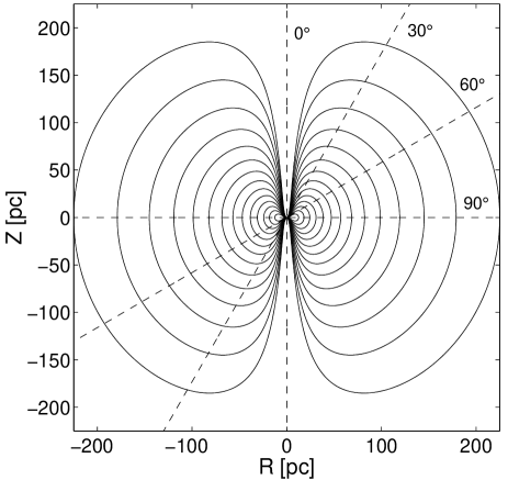
Figure 8: Inclination angle study for our standard model: a) SEDs of the dust re-emission. The inclination varies from 0 °  (upper curve) to 90 °  (lowermost curve) in steps of 10 ° . b) Illustration of some inclination angles of lines of sight frequently used for our standard model.

In Fig. 8a we show an inclination study for SEDs. The uppermost curve belongs to an angle of 0 °, which corresponds to an extreme Seyfert I case, where we see the torus face-on. Typical inclination angles of Seyfert I galaxies are between 10 °and 20 °. Then, the inclination angle is increased up to 90 °, the edge-on case, in steps of 10 °. Some of the inclinations are visualised in Fig. 8b for the case of our standard model. Only dust re-emission SEDs are shown, which result in the so-called IR bump. It arises from dust at different temperatures within the toroidal distribution. The two characteristic silicate features at $9.7\,\muup$m and $18.5\,\muup$m are present in the SED. The $18.5\,\muup$m feature is less pronounced and partially hidden in the global maximum of the IR bump. Just looking at the continuum spectrum and neglecting the silicate bands for a second, an offset in the flux is visible. This offset (explained in Sect. 3.1 and visualised in Fig. 5) is again due to the offset in the extinction curve (see Fig. 3a) and especially visible for the case of silicate grains.

For $i=0\,\degr$, we directly see the torus and the primary source and, therefore, expect the silicate feature in emission. Moving to higher inclination angles, the extinction to occur along the line of sight, mainly caused by cold dust in the outer part of the torus, increases. Less and less of the hotter, directly illuminated parts of the torus can be seen directly. Therefore, the silicate feature changes from emission to absorption. With rising extinction along the line of sight, the increase of the SEDs at small wavelengths is shifted to longer wavelengths and the IR bump gets more and more narrow. The increase at small wavelengths can be explained by a Planck curve with the highest occuring dust temperatures (at the very inner end of the cusp) altered by rising extinction along the line of sight. For our modelling, the torus gets optically thin between 40 and $50\,\muup\mathrm{m}$ (due to the steep decrease of the extinction curve, compare to Fig. 3a). Therefore, all curves coincide and the dust configuration emits radiation isotropically for longer wavelengths.

When we look at the extinction in the visual wavelength range plotted against the inclination angle, $A_{\mathrm{V}}$ reaches about 5 at an inclination angle of 10°. This means that the opening angle of our torus model is too small compared to simple estimates of the torus opening angle using the ratio between Seyfert I and II galaxies, e. g. Osterbrock & Shaw (1988) find a half opening angle between 29°and 39°.

3.4 Inclination angle study for surface brightness distributions

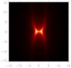
Figure 9: Surface brightness distributions of our standard model with an isotropically radiating central source (first row) and with a $\left|\cos\theta\right|$ - radiation characteristic (second row) at inclination angles of 0 °, 30 °, 60 °  and 90 °  given with a linear colour scale ranging from 0 to the maximum value of the respective image.

In the following section, an inclination study for surface brightness distributions is presented. The underlying model is our standard model introduced earlier. As wavelength we chose $\lambda$ = $13.18\,\muup\mathrm{m}$, which lies in the continuum spectrum outside the silicate feature and still belongs to the wavelength range covered by MIDI (Leinert et al. 2003). Using the Wien law as a rough estimate of the temperature, where the dust emits the maximal radiation at this wavelength, we get about 230 K. Looking at the steep radial temperature distributions of the various grains (see Fig. 7b), we expect the radiation to come from the direct vicinity of the inner radius of the torus. The resulting surface brightness distributions for inclination angles of 0 °, 30 °, 60 °  and 90 °  are shown in the upper row of Fig. 9. The images are given in a linear colour scale emphasising areas of maximum surface brightness. The axis labeling denotes the distance to the centre of the AGN in pc. When we consider flux scales, the object is always assumed to be at a distance of 45 Mpc, which is a typical value for Seyfert galaxies, which will be observed with MIDI.

Looking at the image with an inclination angle of 90 °(the last image in the first row of Fig. 9), the most central part of the torus funnel is visible. As already mentioned above, the dust species sublimate at different distances from the central source. Within these inner radii, no such grains can survive. Therefore, a layering of dust grains exists in the vicinity of the cusp. This is partly visible here. While the very inner end of the torus appears quite faint due to the depletion of many grain species (especially the most abundant small silicate grains and also the smallest graphite grains), a semilunar feature is visible further out. At this point, the dust density increases strongly, because the sublimation radii of small silicate grains are reached. They provide the highest mass fraction of all dust species (for this dust model, the two smallest silicate grain populations carry about 43% of the total mass). Apart from this, an x-shaped emission area appears. Here we see the directly illuminated funnel walls. As the dust density peaks further out at a distance of 5 pc in the equatorial plane, the dust density next to the funnel (outer equipotential lines) is quite low. Hence, only an x-shaped feature remains from the emission of the walls, which arises from a summation effect along the lines tangential to these walls of the funnel. The two maxima are connected via an emission band, which gets fainter and more narrow towards the centre, again due to a summation effect, which is stronger for the case of a line of sight tangential to the ring than perpendicular.
At an inclination angle of 60 °, the same features remain, but the two semilunar areas of maximal emission get connected via thin and faint bows, due to the different line of sight to the ring-like structure. This effect further increases at $i$ = $30$ °. Now, the whole ring of the main dust grain contributors is visible. We see here the intersection of the sublimation sphere of these kind of grains with the torus.

In the face-on case ($i$ = $0$ °), we get the expected ring-like structure. In the central area no emission is present, because in our modelling the funnel of the dusty torus itself is free of any material. The maximum surface brightness does not result from the innermost part of the torus – although these dust grains possess the highest temperatures – because of the summation effect already mentioned above. Only very little dust can exist here because of the density model itself and because the sublimation radii of the main dust contributors lie further out. Summing up along the line of sight results in the shown distribution of surface brightness.

3.5 Wavelength study for surface brightness distributions

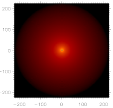
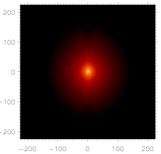
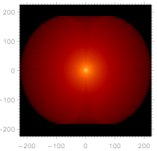
Figure 10: Surface brightness distributions of our standard model for different wavelengths from left to right ($7.22\,\muup\mathrm{m},\,9.7\,\muup\mathrm{m},\,13.18\,\muup\mathrm{m},\,30.2\,\muup\mathrm{m}$). Maps are given in logarithmic scale for inclination angles of $i$ = $0\,\degr$ (upper row) and $i$ = $90\,\degr$ (lower row). See text for a detailed description.

In Fig. 10 we show surface brightness distributions at different wavelengths for the face-on and the edge-on view on our mean Seyfert torus model. Images for the same inclination angles are given with the same logarithmic colour scale and a dynamic range between the global maximum at the respective inclination angle and $10^{-3}\%$ of this value. Again, only re-emission spectra of the dust configuration are shown. The direct radiation of the energy source is neglected. When we would take this into account, the centre would always yield the highest brightness in the surface brightness distribution. The wavelengths are chosen as follows: We start with $7.22\,\muup\mathrm{m}$, located outside the silicate feature at $9.7\,\muup\mathrm{m}$, but closest to $8\,\muup\mathrm{m}$, where the wavelength range of the MIDI (Leinert et al. 2003) instrument starts. The next is the wavelength of the feature itself, then between the two silicate features (at $13.18\,\muup\mathrm{m}$) at the upper end of the MIDI wavelength range and finally we chose the overall maximum of the SEDs ($30.2\,\muup$m).

At wavelengths smaller than approximately $2\,\muup\mathrm{m}$, re-emission of dust can be neglected and pure emission of the central source remains, attenuated by the dust. The surface brightness distributions at varying wavelengths highlight explicitly the different temperature domains. According to Wien’s law, the maximum surface brightness at a wavelength of about $7\,\muup\mathrm{m}$ is emitted by dust of a temperature of around $400\,$K. This area is concentrated to the innermost part of the dust distribution, caused by the very steep radial temperature curve there. Dust heated to about $100\,$K – which is reached in the flattening part of the temperature distribution – has its maximum radiation at a wavelength of around $30\,\muup\mathrm{m}$. Therefore, emission can be seen from a large fraction of the torus volume. The same behaviour is also visible in the case of an inclination of $90\,\degr$. While for small wavelengths basically the x-shaped structure is visible, at longer wavelengths one can see the whole torus. This is also due to the fact that the extinction curve drops off very steeply and, therefore, we expect emission from all over the torus body.

3.6 Implementation of a radiation characteristic

Figure 11: Comparison of the temperature distribution of our standard model (solid lines) with the model with an anisotropically radiating accretion disc (dotted lines). The respective pairs of radial temperature distributions for the smallest silicate grain component are shown. From left to right: within the equatorial plane, for an inclination angle of 30°and an inclination angle of 20°.

Figure 12: SEDs at inclination angles of 0 °  and 90 °  for our standard model with an isotropically radiating accretion disc (given by the solid line) and for the same model but with an accretion disc with a $|cos(\theta)|$ - radiation characteristic, without zoom (dotted line) and zooming into the inner 10 pc in radius (dashed line).

A further step towards a more physical model was the introduction of a radiation characteristic of the accretion disc (see also Manske et al. (1998)). We wanted to check if this yields less steep radial temperature distributions, helping us to explain the increasing depth of the silicate feature seen in correlated flux measurements performed by MIDI (Jaffe et al. 2004). In an extended optically thick accretion disc, a significant part of the radiation arises from the surface. Therefore, in a simple approach, we implemented a radiation characteristic following the same $|\cos(\theta)|$ law for all wavelengths. After emission of a photon package from the central source, the direction of emission is chosen by chance, but in accordance with this radiation characteristic.

In Fig. 11, the differences in the temperature distributions of the smallest silicate dust component are visualised. Here, one can directly see that compared to the isotropic radiating case, the $|\cos(\theta)|$ characteristic for the photon emission leads to hotter areas near the funnel walls, while the temperature within the equatorial plane gets lower. This is understandable, because the midplane is mainly heated by indirect reradiation of the dust in this case.

In Fig. 12, SEDs of our standard model with an isotropically radiating accretion disc (given by the solid line) are compared to the case of an accretion disc with a $\left|\cos\theta\right|$ - radiation characteristic (dotted line). The dashed line corresponds to the model with a radiation characteristic, but zoomed into the central 10 pc in radius and will be discussed in Sect. 3.10. As the maximum dust temperature is smaller when implementing a radiation characteristic, the left branch of the IR bump is slightly shifted to longer wavelengths. The dotted line coincides here with the dashed line. With increasing inclination, this effect gets less important due to increasing extinction along the line of sight. In disagreement with Manske et al. (1998), we cannot find any change of the depth of the silicate feature, when comparing the SED with an isotropically radiating accretion disc with the anisotropic case. This is caused by the different geometry in the innermost part of the torus and other values of the optical depth of our modelling compared to their approach. The cusp of the torus, which is only present in our modelling leads to a more pronounced silicate feature in emission for small inclination angles.
In the second row of Fig. 9, surface brightness distributions at different inclination angles are shown for the case of our standard torus model, illuminated by the accretion disc described above. Here, one can directly see that the radiation characteristic leads to an enhanced heating of the funnel walls. This is best seen when comparing the images at an inclination angle of $0\,\degr$. The area of maximum emission increases for the case of an implemented radiation characteristic, because more energy is emitted into the relevant solid angle and can, therefore, heat the funnel efficiently up to a larger height. In contrast to this, the equatorial plane can only be heated by reemitted photons and, therefore, only smaller temperatures are reached. This effect is visible directly when looking at the image for the edge-on view to the torus. The midplane appears as a narrow absorption band.

3.7 Dust mass variation study for SEDs

Figure 13: SEDs at inclination angles of 0 °  and 90 °  for different optical depths along an equatorial line of sight: $\tau_{9.7\,\muup\mathrm{m}}$ = $4.0$ (dotted line), $\tau_{9.7\,\muup\mathrm{m}}$ = $2.0$ (solid line – our standard model ), $\tau_{9.7\,\muup\mathrm{m}}$ = $1.0$ (dashed line) and $\tau_{9.7\,\muup\mathrm{m}}$ = $0.5$ (dashed-dotted line).

To study the impact of changing the dust mass, which is enclosed in the torus, we started with our standard model (given by the solid line in Fig. 13) with an optical depth of $\tau_{9.7\,\muup\mathrm{m}}$ = $2.0$, doubled the mass (dotted line, $\tau_{9.7\,\muup\mathrm{m}}$ = $4.0$) and halved it twice (dashed line with $\tau_{9.7\,\muup\mathrm{m}}$ = $1.0$ and dashed-dotted line with $\tau_{9.7\,\muup\mathrm{m}}$ = $0.5$). The resulting SEDs are shown in Fig. 13 for the Seyfert I and Seyfert II case with inclination angles of 0 °  and 90 °  respectively. As the optical depth is given by the integral of the product of the dust density and the mass extinction coefficient along the line of sight, it scales linearly with the enclosed dust mass:

$$\tau_{\mathrm{ext}}=\int_{\zeta}\limits\rho_{\mathrm{d}}\,\kappa_{\mathrm{ext}}\,ds.$$ (10)

When we choose a line of sight within the dust-free hole of the torus – corresponding to the Seyfert I case – the whole temperature range of the dust in the torus can be seen. With increasing optical depth, more and more photons are absorbed within a decreasing volume near the funnel of the torus and reemitted in the infrared wavelength range. This leads to a rise of the temperature of dust near the funnel. But due to the high optical depths, less photons reach the outer part of the torus and, therefore, the temperature drops. Altogether, a steeper temperature distribution in radial direction results. Smaller minimum temperatures lead to a shift of the Rayleigh-Jeans branch to longer wavelengths and larger maximum temperatures lead to a shift of the Wien branch to shorter wavelengths. Altogether, the IR bump gets broader. The higher temperatures in the inner region also cause more flux at short wavelengths, while the larger amount of cold dust produces more flux at longer wavelengths. The global maximum of the IR bump is shifted to higher wavelengths because of the smaller temperatures at the point of the maximum of the dust density.

For an inclination angle of 90 °, which corresponds to a Seyfert II-like case, there is always dust on the line of sight. Only the outer and, therefore, the coldest part of the torus can be seen directly. That is why we can use the reasoning for the Seyfert I case for the long wavelength region. The innermost (and therefore hottest) part of the torus can only be seen through an increasing amount of dust. The higher the extinction the less we can look into the torus and the less hot areas of the torus can be seen. Therefore, the left branch of the IR bump is shifted to higher wavelengths when the extinction increases. The $9.7\,\muup\mathrm{m}$ silicate feature changes from emission over partial absorption to total absorption, comparable to large inclination angles in the study shown in Sect. 3.3. As discussed above, increasing dust mass affects the optical depth linearly. When $\tau$ = $1$ is reached, the torus gets optically thick, and, therefore, the feature changes from emission to absorption. Between these two cases, a smooth transition region is visible, where the feature can be seen in partial absorption and emission, called self-absorption (Henning 1983). Intersecting the $\tau$ = $1$ line with the optical depth plotted against the wavelength though displays the expected behavior of the silicate feature in the spectrum. The same holds for the second silicate feature at $18.5\,\muup\mathrm{m}$ but in alleviated form as it is much weaker and partially covered by the global maximum of the IR bump.
The study shows that the SEDs are very sensitive to changes in the dust mass. Already a change by a factor of four changes the feature from emission to complete absorption (see solid line compared to dashed-dotted line in Fig. 13). Therefore, the silicate feature is a quite sensitive tool to distinguish the optical depth along the line of sight.

3.8 Dust mass variation study for surface brightness distributions

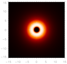
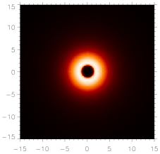
() $\tau_{9.7\,\muup\mathrm{m}}$ = $0.5$

() $\tau_{9.7\,\muup\mathrm{m}}$ = $1.0$

() $\tau_{9.7\,\muup\mathrm{m}}$ = $4.0$

() $\tau_{9.7\,\muup\mathrm{m}}$ = $8.0$

Figure 14: Surface brightness distributions at a wavelength of $\lambda$ = $13.18\,\muup$m for models with different optical depths. The values for the optical depth are $\tau_{9.7\,\muup\mathrm{m}}$ = $0.5$ (left column), $\tau_{9.7\,\muup\mathrm{m}}$ = $1.0$, $\,\tau_{9.7\,\muup\mathrm{m}}$ = $4.0$ and $\tau_{9.7\,\muup\mathrm{m}}$ = $8.0$ (right column) and inclination angle changes from 0 °  (upper row) to 90 °  (lower row) in steps of 30 °. Each step in $\tau$ means doubling the included dust mass. The images with $\tau_{9.7\,\muup\mathrm{m}}$ = $2.0$ are omitted (please compare to Fig. 9). All images are given with a linear colour scale reaching from zero to the maximum of the respective image.

Figure 15: Cut through the surface brightness distributions $\mu_{\nu}$ at a wavelength of $\lambda$ = $13.18\,\muup$m along the positive x-axis for inclination angles of 0 °  and 90 °. The thick solid line corresponds to the case with $\tau_{9.7\,\muup\mathrm{m}}$ = $0.5$, the thin solid line to $\tau_{9.7\,\muup\mathrm{m}}$ = $1.0$, the dotted line to our standard model with $\tau_{9.7\,\muup\mathrm{m}}$ = $2.0$, the thick dashed line to $\tau_{9.7\,\muup\mathrm{m}}$ = $4.0$ and the thin dashed line to $\tau_{9.7\,\muup\mathrm{m}}$ = $8.0$. The fluxes shown are given in Jansky per square milliarcsecond for an assumed distance of the object of 45 Mpc.

To study the impacts of changing the optical depth along the line of sight on surface brightness distributions, we used the same dust masses as in Sect. 3.7 for the case of spectral energy distributions to gain comparability, but doubled the highest mass again. This means that coming from our standard model, we doubled the enclosed dust mass twice and halved it twice. Again, we chose the same wavelength of $13.18\,\muup\mathrm{m}$. The results are shown in Fig. 14. The different optical depths ($\tau_{9.7\,\muup\mathrm{m}}$ = $0.5$, $\tau_{9.7\,\muup\mathrm{m}}$ = $1.0$, $\tau_{9.7\,\muup\mathrm{m}}$ = $4.0$, $\tau_{9.7\,\muup\mathrm{m}}$ = $8.0$) are shown in different columns, while the inclination angle changes are shown in different rows, starting from 0 °  in the upper row to 90 °  in the lower row. Our standard model is omitted here, please compare to Fig. 9. All of the images are given in a linear colour scale, with a dynamic range between zero and the maximum value of the respective map in order to show the changes in the distribution of maximum surface brightness for the different optical depths. The absolute values for the pixels are given in Fig. 15, which shows a cut through the maps of the dust mass variation study from the centre along the positive x-axis for an inclination of 0 °  and 90 °. The fluxes are given in Jansky per square milliarcsecond for an assumed distance of the object of 45 Mpc. For the case of 0 °, all graphs show the same trend: coming from the centre, one can see a sharp rise of surface brightness with a sharp peak and a flatter decrease in the outer part. Between 4 and 5 pc, all of the curves meet into a single curve, independent of the optical depth. The latter is due to the fact that our model features very steep funnel walls. As indicated by the temperature distribution, we expect most of the emission for this wavelength next to the torus boundary. The intersection of all curves then indicates the distance from the centre, where the density has decreased that much that a doubling of it does not change the emitted flux anymore and the expected surface brightness distribution is independent of the optical depth within our sample. By increasing the optical depth, the maximum is shifted towards the centre and to higher values and the curves get steeper. As already discussed in the previous section, the higher the optical depth is the steeper the drop of the temperature distribution in radial direction is, because the photon mean free path length decreases and most of the photon packages get absorbed within a reduced volume of the dust torus (steepening of the inner part) and, therefore, only reemitted photons in the IR reach the outer region (flattening of the outer part). To estimate the surface brightness, one has to take into account all emission by dust until $\tau$ = $1$ is reached. This can also be directly seen in Fig. 14 in the decreasing size of the region of maximum emission. The apparent shift of the inner radius of the torus is caused by the increase of the atmosphere around the dense core of the torus or the growth of the denser core, respectively.

At the other inclination angles one can again see that the area of maximal emission changes. At smaller optical depths, it is a diffuse, wide distribution within the torus volume. Increasing the optical depth leads to a spreading, which is more located in the direct vicinity of the inner funnel border. This leads to the sharply emerging inner borders of the funnel, which are now visible in the typical x-shaped form. These appearances have been seen in a similar dust configuration around a double system, the so-called Red Rectangle (Tuthill et al. 2002), which can be explained by a dusty torus as well (Men’shchikov et al. 2002). It is located in a distance of only 330 pc, much closer than Seyfert galaxies and can therefore be resolved.

At higher inclination angles, two effects have to be taken into account. With increasing amount of dust along the line of sight, first of all, we expect a larger surface brightness, but the extinction along the line of sight increases as well. The value of the maximum of the cut along the positive x-axis of the maps with the highest optical depth is not the brightest anymore. It decreases with increasing inclinations. In Fig. 15b the case for an inclination angle of 90 °  is shown. Here, the model with the highest dust mass (thin dashed line) has the smallest surface brightness and the curve of the second heaviest torus (thick dashed line) has also shifted significantly to smaller values. The shape of these graphs also changes when changing from the Seyfert I ($i$ = $0$ °) case to the Seyfert II ($i$ = $90$ °) case. As the directly illuminated parts of the funnel are not directly visible anymore, the decreasing curve further away from the centre decreases faster. With increasing optical depth, the outer part of the torus gets colder and colder, which can be seen by the decreasing flux and the steepening of the curves there. In the innermost part, the curves flatten, which is due to the emission band of the innermost ring of the funnel. As less photons reach the outer part, statistic gets poorer there and therefore the graphs get more noisy.

Figure 16: Optical depth within the equatorial plane for different dust models: a Increasing the exponent of the number density distribution of grain sizes, from $-3.5$ (our standard model, given by the solid line) over $-3.0$ (dotted line) and $-2.5$ (dashed line) to $-2.0$ (dashed-dotted line). b Changing the range of grain sizes, from $0.005\dots 0.25\,\muup$m (our standard model, given by the solid line) to $0.005\dots 10\,\muup$m (dotted line) and to $0.001\dots 10\,\muup$m (dashed line).

3.9 Variation of dust properties

As already pointed out in Sect. 2.3, the dust composition in the extreme environment of an AGN may be altered compared to interstellar dust in our own galaxy. The main effects here are sputtering due to interaction of the dust grains with the hot surrounding gas, the presence of the strong radiation field of the central source, destruction of dust grains due to shocks, etc.

All of the mentioned effects mainly impact the population of small grains. Therefore, some authors (e. g.  Laor & Draine 1993; Maiolino et al. 2001) claim that within an AGN dust model, small grains should be depleted. In the following section, we test this by first of all changing the exponent of the number density distribution of grain sizes and later by widening the grain size distribution in both directions. By doing this, a transition is made between the standard MRN galactic dust model – which we have adopted as our standard dust model – and the dust model proposed by van Bemmel & Dullemond (2003). In this section, we are especially interested in the behaviour of the $9.7\muup$m silicate feature, as it was claimed that the depletion of smaller grains may solve the problem that the feature is never seen in emission in AGN. On the other hand one needs to check whether other constraints are violated by this change of the dust model, e. g. the appearance of the feature in absorption, as observed.

3.9.1 Changing the exponent of the number distribution of grain sizes

Different exponents of the number density distribution of the grains were tested by van Bemmel & Dullemond (2003) for their torus model. They finally adopt a somehow more shallow distribution with an exponent of $-2$ to be their standard dust model.

In this section, we also check different slopes of the distribution for our standard torus geometry (see Sect. 2.2). We start with our standard dust model with a slope of $-3.5$ (given by the solid line in Fig. 16a and Fig. 17) and test shallower distributions by changing the exponent in steps of $0.5$ up to $-2.0$ (dashed-dotted line) used by van Bemmel & Dullemond (2003). Due to renormalisation of the dust density after changing the exponent, this means that a flatter distribution leads to more large grains compared to small grains. This produces a flatter course of the optical depth (see Fig. 16a) at small wavelengths – compared to our standard model – because of the less efficient heating of larger grains, which dominate the dust composition more and more during the variation. Consequently, the temperature distributions flatten.

In the SEDs (see Fig. 17a), this can be seen by the decreasing fluxes at the rise of the IR-bump at small wavelengths and the increasing fluxes at wavelengths around the maximum ($20-30\muup$m) of the infrared bump (see Fig. 17a). The stratification of dust grains concerning sizes and composition and the increasing extinction caused by the large grain population (with smaller sublimation radii) lead to larger sublimation radii for the other components. In contradiction to the modelling of van Bemmel & Dullemond (2003), a significant change of the silicate feature cannot be found in our simulations. For the case of an inclination angle of $90\degr$ (see Fig. 17b), any change is simply due to the fact that there is too little dust left that has temperatures higher than about $300$K – the temperature which is required for the emission feature at $9.7\muup$m.

Figure 17: Consequences on the SEDs at inclination angles of $0\degr$ and $90\degr$ of changing the exponent of the dust grain number density distribution. The exponent changes from $-3.5$ (solid line) in steps of $0.5$ to $-2.0$ (dashed-dotted line).

Figure 18: Consequences on the SEDs at inclination angles of $0\degr$ and $90\degr$ of changing the width of the dust grain size distribution from $0.005\dots 0.25\,\muup$m (solid line) over $0.005\dots 10\,\muup$m (dotted line) and finally to $0.001\dots 10\,\muup$m (dashed line).

3.9.2 Changing the width of the grain size distribution

In a further dust parameter study, we test the effects of a broadening of the grain size distribution. The corresponding courses of the optical depths with wavelength within the equatorial plane are plotted in Fig. 16b and the resulting SEDs in Fig. 18b. Starting from the MRN model (given by the solid line), we first extend the grain size range towards larger grains (dotted line) up to $10\muup$m size and later additionally towards smaller grains down to $0.001\muup$m (dashed line). By doing this, we finally get the dust model used by van Bemmel & Dullemond (2003).

As can be seen from Fig. 16b, only minor changes of the optical depth are visible. Conspicuous is the smaller relative depth of the silicate feature towards shorter wavelengths after including also large grains (dotted line). This can also be seen in the SEDs, displayed in Fig. 18b. While the differences for an inclination angle of $0\degr$ are nearly negligible, the reduced relative depth of the silicate feature towards smaller wavelengths is clearly visible in the SED for edge-on view ($i=90\degr$). In the last step of our study – the inclusion of pronounced slightly smaller grains – the effects of extending the size distribution towards larger grains is partly compensated.

3.10 Zooming into the torus

Figure 19: Dependence of SEDs on the beamsize of the observing device. The solid line corresponds to our standard model, the dotted line to the resolution obtainable with a single-dish telescope (100 mas) for a distance to the object of 45 Mpc and the dashed line to the resolution of the MIDI interferometer (10 mas). The left panel shows SEDs for an inclination angle $i=0\,\degr$ and the right panel for $i=90\,\degr$.

Another simulation series we made was to investigate the impact of zooming into the torus resembling a certain aperture of the telescope. To do this, we again started from our standard model and zoomed into the central 10 pc and 1 pc in radius. This corresponds to a resolution of the observing instrument of 100 mas and 10 mas for an object at a distance of 45 Mpc. These are typical values for the largest single-dish telescopes (100 mas) and the first interferometers in this wavelength range like MIDI (10 mas). The results of this study are shown in Fig. 19. In terms of surface brightness distributions compare to Fig. 9.

When we decrease the aperture, we concentrate more and more on the central parts of the torus emission. As our temperature distribution is very steep, it is expected that cold dust in the outer part of the torus is excluded from the field of view. Therefore, the smaller the aperture, the less total flux we obtain, which is taken from the large wavelengths part of the spectrum. For the case of 10 mas resolution, only the inner pc in radius is visible. This is even less than the sublimation radius of the smallest silicate grains (approximately 1.3 pc).

For the silicate feature, one notices a decrease of the relative depth rather than the expected increase, as seen with MIDI (compare to Fig. 2 in Jaffe et al. (2004)). This might be due to a too steep radial temperature distribution of our models. Introducing a cloudy structure, which leaves unobscured channels up to the outer part of the torus, may lead to a direct heating of clouds further outside and therefore to a broader temperature distribution. Zooming into the centre then means for the Seyfert II case to exclude areas, where emission features are produced and a deepening of the silicate absorption feature is expected to take place.

4 Comparison with observations

In this section, simulated spectral energy distributions are compared to available observational data for the case of large aperture SEDs and high spatial resolution SEDs.

4.1 Comparison with large aperture spectra of type I galaxies

Figure 20: Comparison of our standard model (different line styles correspond to varying dust masses) with large aperture spectra for type I objects. Plus signs refer to 29 radio quiet quasars (Elvis et al. 1994), squares to 16 Seyfert I galaxies (Granato & Danese 1994) and diamonds and triangles to PG Quasars (Sanders et al. 1989) with luminosity smaller (diamonds) and larger (triangles) than $10^{12}\,L_{\sun}$. For a typical Seyfert I galaxy ($10\,\degr<i<20\,\degr$), the silicate feature looks much less pronounced (see Fig. 8a).

In Fig. 20 we compare the resulting SEDs of our standard model (different line styles) for an axial view on the torus (typically, Seyfert I galaxies have inclination angles between 10 °and 20 °) with varying enclosed dust masses (as described in Sect. 3.7 and shown in Fig. 13) to different sets of mean large aperture data for type I objects. The plus signs refer to a mean spectrum, extrapolated from 29 radio quiet quasars, provided by Elvis et al. (1994), the squares correspond to 16 Seyfert galaxies, reported by Granato & Danese (1994). Triangles and diamonds represent radioquiet type I PG quasars with bolometric luminosity larger and smaller than $10^{12}\,L_{\sun}$ respectively (Sanders et al. 1989). All of these data sets are scaled in order to get fluxes comparable to our simulations.

As can be seen from this, our models compare well to the overall shape of the UV to FIR wavelength range of these mean AGN spectra. An exeption is the pronounced feature at $9.7\,\muup$m. As already discussed before, it has never been observed in emission in SEDs of Seyfert galaxies – as well not in SEDs of higher spectral resolution. The introduction of a clumpy structure of the dust distribution, which is also a more physical solution, might help to remove these large emission features of our models. A comparison with high spatial resolution SEDs of type II sources is given in the next section for some selected objects.

4.2 Comparison with special Seyfert II galaxies

To specify as many of our simulation parameters as possible for these special objects, we started with a literature study. Some of the remaining variables could be chosen according to conditional relations as mentioned in Sect. 2.2. The value of the enclosed dust mass was assumed such that the relative depth of the $10\,\muup$m-feature appears comparable to the observations of the correlated flux with a baseline of 78 m done with MIDI for the case of NGC 1068 and comparable to the depth of the feature in the MIR spectrum of Roche et al. (1991) for the Circinus galaxy. As zooming into our torus does not reproduce the deepening of the silicate feature as seen by MIDI, this seems to be a reasonable procedure and explains the deviations concerning wavelengths around the feature for the case of NGC 1068. It results in an optical depth in the equatorial plane at $9.7\,\muup$m of $\tau$ = $3.3$ for NGC 1068 and $\tau$ = $3.9$ for the Circinus galaxy. The free parameters finally were chosen to obtain a reasonable dust distribution and a good comparison with the data.

4.2.1 NGC 1068

NGC 1068 is a nearby Seyfert II galaxy at a distance of 14.4 Mpc (Galliano et al. 2003). Therefore, it has been studied extensively and we were able to find at least some of the needed simulation parameters in literature. The procedure described above led to the parameters summarised in Table 2. The inclination angle of $i=85$ °  was chosen in agreement with the tilt of the outflow cone of ionised gas reported by Crenshaw & Kraemer (2000). For our comparison, we use a compilation of high resolution data done by M. A. Prieto, given in Table 3. Fig. 21 shows the result of the adaptation of the model given in Table 2 to this data set. The line corresponds to a zoomed-in view of the torus by a factor of 10, which resembles the aperture of 0.2″in diameter of most of the datapoints (given by the triangles) in Fig. 21. The diamonds correspond to a slightly larger aperture of 0.27″. The L-band flux, which corresponds to an aperture of 0.7″in diameter is given by the square symbol. In addition, we added the total flux (dashed-dotted line) – corresponding to an aperture of $0.6\,\times 0.6\arcsec$ – and the correlated flux spectrum for a baseline of 78 m (dotted line) – corresponding to an aperture in diameter of approximately $30\,mas$ (Jaffe et al. 2004). As can be seen in this figure, observations are in good agreement with our model except of the wavelength region around the $9.7\,\muup$m silicate characteristic. As already mentioned before, zooming into our model torus does not reproduce the trend of MIDI-observations, which means a deepening of the silicate feature. We therefore adapted the depth of our feature to the depth observed in correlated flux measurements of MIDI with a baseline of 78 m. This was also necessary in order to describe the datapoints at the smaller wavelengths.

Table 2: Parameters used for the simulation of NGC 1068.

Parameter	Value	Reference
$M_{\mathrm{BH}}$	$8.3\cdot 10^{6}\,M_{\sun}$	Greenhill et al. (1996)
$R_{\mathrm{c}}$	24 pc	Gallimore & Matthews (2003)
$M_{*}$	$6.5\cdot 10^{8}\,M_{\sun}$	Thatte et al. (1997)
$L_{\mathrm{disc}}$	$5.42\cdot 10^{10}\,L_{\sun}$
$L_{\mathrm{disc}}/{L_{\mathrm{Edd}}}$	20%
$R_{\mathrm{T}}$	3 pc
$M_{\mathrm{dust}}$	$7.8\cdot 10^{4}\,M_{\sun}$
$\tau_{9.7\,\muup\mathrm{m}}$	3.3
$R_{\mathrm{out}}$	72 pc
$v_{\mathrm{t}}$	$164\,\mathrm{km}\,\mathrm{s}^{-1}$
$\gamma$	0.5
$d$	14.4 Mpc	Galliano et al. (2003)
$i$	85 °	Crenshaw & Kraemer (2000)

Figure 21: Comparison of one of our models (described by the parameters given in Table 2 and plotted with a solid line) to a set of data (given in Table 3) from high spatial resolution observations of NGC 1068, compiled by M. A. Prieto. The various symbols correspond to slightly different apertures. The dashed-dotted line gives the total flux spectrum obtained with MIDI and the dotted line corresponds to the correlated flux spectrum obtained with MIDI for a baseline of 78 m (Jaffe et al. 2004).

Table 3: High resolution data of NGC 1068. The compilation was done by M. A. Prieto. The references are R98 (Rouan et al. 1998), P04 (Prieto, private communication), M03 (Marco & Brooks 2003) and B00 (Bock et al. 2000).

Wavelength	Band	Flux	Aperture (dia)	Reference
$\muup$m		Jy	arcsec
1.30	J	5e-4	0.20	R98
1.70	H	6e-3	0.20	R98
2.20	K	5.6e-2	0.27	P04
3.79	L	1.5	0.70	M03
4.47	M	2.5	0.27	P04
7.99	N	4.23	0.20	B00
9.99	N	3.33	0.20	B00
11.99	N	7.1	0.20	B00
24.98		9.4	0.20	B00

4.2.2 Circinus

The Circinus galaxy is one of the nearest spiral galaxies, which harbors an Active Galactic Nucleus. As it is the second extragalactic object, which has been observed by MIDI and also with NAOS/CONICA (Prieto et al. 2004), we also carried out a comparison with one of our models. From the first results of these observations (Prieto et al. 2004) and also from previous modelling of the dusty torus by Ruiz et al. (2001), we know that it harbors a relatively small sized toroidal dust distribution. Therefore, we used a scaled down version of our standard model described above. The simulation was done with the parameters summarised in Table 4.

Figure 22: Model comparison with high spatial resolution data of the Circinus galaxy taken with the NACO camera at the VLT. Data courtesy of Prieto et al. (2004). The data was corrected for foreground extinction by $A_{\mathrm{V}}$ = $6\,\mathrm{mag}$. The various symbols correspond to different apertures (see Table 5).

Table 4: Parameters used for the simulation of the Circinus galaxy.

Parameter	Value	Reference
$M_{\mathrm{BH}}$	$1.7\cdot 10^{6}\,M_{\sun}$	Greenhill et al. (2003)
$R_{\mathrm{c}}$	10 pc
$M_{*}$	$2.0\cdot 10^{8}\,M_{\sun}$
$L_{\mathrm{disc}}$	$8.4\cdot 10^{9}\,L_{\sun}$,
$L_{\mathrm{disc}}/{L_{\mathrm{Edd}}}$	15%
$R_{\mathrm{T}}$	3.5 pc
$M_{\mathrm{dust}}$	$2.0\cdot 10^{4}\,M_{\sun}$
$\tau_{9.7\,\muup\mathrm{m}}$	3.9
$R_{\mathrm{out}}$	30 pc
$v_{\mathrm{t}}$	$140\,\mathrm{km}\,\mathrm{s}^{-1}$
$\gamma$	0.5
$d$	4.2 Mpc	Freeman et al. (1977)
$i$	90 °	Crenshaw & Kraemer (2000)

Table 5: High resolution data of the Circinus galaxy. The data was corrected for foreground extinction by $A_{\mathrm{V}}$ = $6\,\mathrm{mag}$. Data courtesy of Prieto et al. (2004).

Wavelength	Band	Flux	Aperture (dia)
$\muup$m		mJy	arcsec
1.30	J	$\la$7.9	0.38
1.70	H	15.0	0.10
2.20	K	36.0	0.38
2.42		54.0	0.38
3.79	L	480.0	0.38
4.47	M	2200.0	0.38
11.80	N	15000.0	1.00

Fig. 22 shows the result of the comparison of this model (given by the solid line plot) with data taken with the NACO camera at the VLT (Prieto et al. 2004). Various symbols represent different apertures (see Table 5). Fluxes, corrected for foreground extinction by $A_{\mathrm{V}}$ = $6\,\mathrm{mag}$, are used.

The graph corresponds to a torus model with an inner radius of approximately 0.9 pc and a luminosity of the central source of 15% of the Eddington luminosity. The modelling leads to a maximum temperature lower than the sublimation temperatures of the dust grains. Models with smaller inner radii and, therefore, higher maximum temperatures can be excluded. For models with higher maximum temperature, the rise of the IR bump at small wavelengths is moved towards smaller wavelengths. In order to avoid this, we would have to increase the amount of dust, leading to a deeper silicate feature, in contradiction to available observations. This shows that sublimation temperatures of the dust grains are only reached in some of the torus configurations. Our model fits well to the observations, except of the small wavelength part of the SED. This excess is not due to torus emission. The increased fluxes are most probable caused by light from the central source, scattered above the torus by material (dust and electrons) within the opening of the torus.

Our attempts to model observational data showed once more the inherent ambiguity: The same SED can be modelled with different parameter sets or even models. Therefore, additional information from observations is needed in order to be able to distinguish between different torus models.

5 Conclusions and outlook

In this paper we present new radiative transfer simulations for dust tori of Active Galactic Nuclei. The dust density distribution and the geometrical shape of the torus model result from a hydrostatic equilibrium in which gravitational and centrifugal forces of the nuclear stellar distribution and the central black hole are balanced by pressure forces due to the turbulent motion of the clouds. Spectral energy distributions (SEDs) and surface brightness distributions are obtained by a fully three-dimensional treatment of the radiative transfer problem.

After fixing as many parameters of the model as possible by observational constraints, we undertake an extensive parameter study by varying dust properties, dust masses and other factors. It shows that our modelling is able to explain mean observed spectral energy distributions (SEDs) for classes of Active Galactic Nuclei as well as for individual objects.

Obviously, the innermost part of the tori close to the central energy source is crucial for the determination of SEDs in the mid-infrared wavelength range. Specifically, we found that any realistic model has to incorporate the fact that sublimation radii for varying dust grain sizes and dust composition differ considerably. Using mean dust characteristics according to the MRN dust model (see Sect. 2.3) instead leads to incorrect temperature distributions and SEDs. Even with this refinement, the model cannot explain the recent interferometric observations of the MIDI instrument, as reported by Jaffe et al. (2004), which show a deepening of the silicate absorption feature in the correlated flux – effectively sampling the central few parsec of the dust distribution. In order to reproduce these results, a temperature distribution shallower than in our model would be required. We find that introducing a $|\cos\theta|$ radiation characteristic for the primary radiation source does not yield significant changes. In a next step, we will introduce a clumpy structure of our dust configuration. Gaps within the dust distribution should then lead to direct heating of clumps in the outer part of the torus and thus producing a shallower mean temperature distribution. Biasing the grain size distribution of the dust towards larger grains as proposed by several authors (e. g.  Laor & Draine 1993; Maiolino et al. 2001) does not yield a reduction of the emission feature of type I objects for the case of our dust density distribution.

With the present examination of the Turbulent Torus Model for dust distributions in AGNs, we made a first step towards the introduction of more physics into the modelling of the torus emission. We demonstrated that a model based on physical assumptions reproduces the SEDs both on kiloparsec and parsec scales as well as previous models in which the shape and size of the dust distribution are free parameters (e.g. Pier & Krolik (1993); Granato & Danese (1994); Manske et al. (1998); Nenkova et al. (2002); van Bemmel & Dullemond (2003) ).

As pointed out in Sect. 2.1, this kind of stationary modelling cannot account for all physical effects present in such an environment. In a further step, hydrodynamic simulations in combination with radiative transfer calculations should enable us to take at least some of these uncertainties into account. The main effects are continuous energy feedback by supernovae explosions and mass injection by stellar winds.

With the first interferometric observations at hand, however, the problem becomes more challenging: the wide range in observable scales from hundreds of parsec down to one parsec requires not only to reproduce global SEDs of the torus but also to describe its shape, structure and temperature stratification correctly. In addition, these detailed observations are an essential step to resolve the ambiguities that are present in current global models of dusty tori in Active Galactic Nuclei.