GZK cutoff distortion due to the energy error distribution shape

Abstract

The development of an ultra high energy air shower has an intrinsic energy fluctuation due both to the first interaction point and to the cascade development. Here we show that for a given primary energy this air shower energy fluctuation has a lognormal distribution and thus observations will estimate that primary energy with a lognormal error distribution. We analyze the UHECR energy spectrum convolved with the lognormal energy error and demonstrate that the shape of the error distribution will interfere significantly with the ability to observe features in the spectrum. If the standard deviation of the lognormal error distribution is equal or larger than 0.25, both the shape and the normalization of the measured energy spectra will be modified significantly. As a consequence the GZK cutoff might be sufficiently smeared as not to be seen (without very high statistics). This result is independent of the power law of the cosmological flux. As a conclusion we show that in order to establish the presence or not of the GZK feature, not only more data are needed but also that the shape of the energy error distribution has to be known well. The high energy tail and the sigma of the approximate lognormal distribution of the error in estimating the energy must be at the minimum set by the physics of showers.
PACs 96.40.De,96.40.Pq

1 Introduction

Detection of cosmic rays arriving at the Earth with energies above $10^{20}$ eV questions the presence of the GZK cutoff [1]. This cutoff determines the energy where the cosmic ray spectrum is expected to abruptly steepen. Cosmic rays with ultra high energies (above $\sim 5\times 10^{19}$ eV) lose energy through photoproduction of pions when transversing the Cosmic Microwave Background Radiation (CMB). As the CMB attenuates ultra high energy cosmic rays (UHECR) on a 50 Mpc scale (or characteristic distance) at $10^{20}$ eV, one can determine it’s production maximum distance. An event of $10^{20}{\rm eV}$ has to be produced within $\sim 100$ Mpc, unless it is a non standard particle [2, 3]. The absence of any powerful source located within this range [4] — that could accelerate a cosmic ray to such an energy — turns the existence of these events into a mystery, the so called GZK puzzle.

The results of two important cosmic ray experiments AGASA [5] and HiRes [6] are not consistent. Not only is the energy spectrum measured by HiRes systematically below the one measured by AGASA, but also the HiRes spectrum steepens around $10^{20}$ eV while AGASA’s spectrum flattens around this energy region. The steepening in the HiRes spectrum may be in agreement with a GZK cutoff, while AGASA’s is thought not to be.

There are many possible ways to understand this discrepancy  [7, 8]. The Pierre Auger Observatory [9] will soon have a statistically significant data sample and will certainly shed light into understanding these events.

In this article we focus on the role of the shape of the error distribution in the energy determination. We show that the intrinsic features of an air shower results in a lognormal error distribution on the energy determination. The minimum standard deviation of this distribution ($\sigma$) is set by physical properties of the shower. If additional errors due to detection – which increases the $\sigma$ – are not kept to minimum, the end of the energy spectrum will be smeared in a way that the GZK feature might not be seen.

Understanding the energy error is crucial in order to determine whether or not the GZK cutoff is present. A lognormal error distribution on the reconstructed primary cosmic ray energy is to be expected due to fluctuations both in the shower starting point as well as from the cascade development [10]. According to simulations by the AUGER collaboration [11] the depth of first interaction affects the rate of development of the particle cascade of the shower which results in a fluctuation of about 15% on the number of muons and about 5% on the eletromagnetic component. Auger also predicts that the number of muons in a proton induced shower increases with primary energy as E^0.85 [11]. The 15% fluctuation will then contribute as a fixed fractional error and the fluctuation on the number of muons on the ground will be $N=(1\pm 0.15)N_{0}(E\,/\,E_{0})^{0.85}$. Therefore one has to add a 15% contribution to the error in estimating the primary energy in addition to the $\sqrt{N}$ error factor. As this shower starting fluctuation error is a percentage of the energy it results in a lognormal error distribution.

There are mainly two ways of determining the energy: ground detectors reconstruct the energy based on the particle density at a certain distance from the shower core and fluorescence detectors which determine the energy through the shower longitudinal profile [6]. The longitudinal profile determines the number of particles in the shower per depth and it is well known to have large fluctuations. As mentioned above, the fluctuations arise both from the shower starting point as well as from the cascade development. The same is expected for the energy determination in ground detectors, since the particle density depends on the number of particles.

The inherent fluctuations and resulting lognormal error distribution will affect crucially the analysis of data collected in ground arrays since their data sample is collected at one particular depth. It does also affect fluorescence data but as the energy reconstruction uses the full longitudinal profile of the shower, there is more potential information to estimate the original energy.

Figure 1 shows the distribution of particles at ground level for $2\times 10^{4}$ simulated showers (using [12]) from $10^{20}$ eV protons. A lognormal fit with $\sigma=0.08$ is superimposed and it is clear that the distribution has a lognormal shape. The same distribution for showers from $10^{18}$ eV protons is shown in Figure 2. The poor fit is due to an excess of simulated events relative to the lognormal at the high end. The standard deviation of the fit is 0.14. Effects due to the errors with asymmetrical and non-gaussian tails are shown in [13].

Figure 1: Distribution of total number of particles at ground level. Ratio of number of particles over average is shown. $2\times 10^{4}$ showers were simulated with the Aires [12] package. Primary particles are $10^{20}$ eV protons and $\langle{\rm N_{part}}\rangle=2.7\times 10^{10}$. Superimposed is a lognormal curve with $\sigma=0.08$.

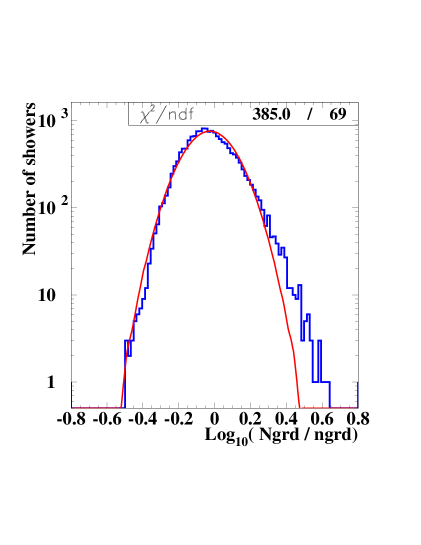
Figure 2: Same as Figure 1 but for $10^{18}$ eV protons as the primaries. Here $\langle{\rm N_{part}}\rangle=14.7\times 10^{7}$. Superimposed is a lognormal curve with $\sigma=0.14$. The poor fit is due to an excess of simulated events relative to the lognormal at the high end.

The simulated showers used Sybill interaction model and assumed that the ground was at sea level (defined in Aires [12] as 0 m or 1036 g/cm²). A more thorough analysis is under way to understand why the error distribution for lower energies (as in Figure 2) deviates from the lognormal shape. However it is clear that most of the events in excess come from the tail of the maximum depth (XMAX) of the shower distribution. In Figure 3 we show the XMAX distribution for the same events used in Figure 2. If we cut events with XMAX $>$ 890 g/cm² from this data set, the ground particles distribution will lose part of the excess events. This distribution is shown in Figure 4. These excess events, if included, would only make more exaggerated the effect we discuss here.

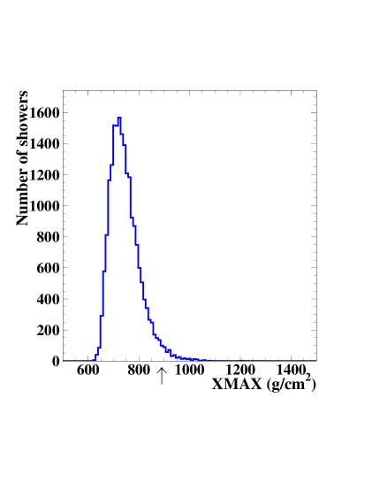
Figure 3: Maximum shower depth (XMAX) distribution for $2\times 10^{4}$ showers with $10^{18}$ eV protons as the primaries. The arrow in the XMAX axis indicates where an analysis cut will be applied.

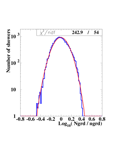
Figure 4: Same as Figure 2 but events with XMAX $>$ 890 g/cm² were removed. Superimposed is a lognormal curve with $\sigma=0.13$. The fit improves in relation to Figure 2.

The results shown in Figures 1 and 2 are also dependent on the location of the ground level. We have also simulated events with ground above sea level at 950 g/cm². The lognormal continues to fit well the $10^{20}$ eV distribution and its $\sigma$ improves to 0.05. The $10^{18}$ eV distribution still has an excess but the chisquare improves to 4 and the $\sigma$ to 0.10.

Below we will describe how we determine the UHECR spectrum assuming a injection power spectrum from cosmologically distributed sources. We account for energy loss due to propagation through the CMB. We then describe how the energy error is evaluated and how it affects the energy reconstruction and the determination of the GZK cutoff.

2 Analytical determination of UHECR propagation and energy spectrum

Our analytical approach assumes a cosmological cosmic ray flux. We assume extragalactic sources isotropically distributed at different redshifts [14]. These sources produce a power law energy spectrum (injection spectrum) which is assumed to be:

$$F(E)=kE^{-\alpha}\exp\left(-\frac{E}{E_{max}}\right)$$ (1)

where $E$ is the cosmic ray energy, $k$ is a normalization factor, $\alpha$ is the spectral index and $E_{max}$ is the maximum energy at the source.

The energy degradation of protons through the CMB includes losses due to pair production [15, 16], expansion of the universe [17] and photopion production [17]. These losses at present epoch are shown in Figure 5.

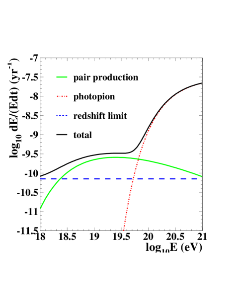
Figure 5: Energy losses (as labeled) of a proton transversing the CMB at present epoch.

We include current values for the matter and dark energy density ($\Omega_{M}$ and $\Omega_{\Lambda}$) when considering the energy loss due to expansion of the universe ($\beta_{z}$):

$$\beta_{z}(E,z)=H_{0}\sqrt{\Omega_{M}(1+z)^{3}+\Omega_{\Lambda}}$$ (2)

where $\beta$ is defined as $\beta=1/E\times dE/dt$ and $\Omega_{M}=0.3$, $\Omega_{\Lambda}=0.7$ and $H_{0}=75$  km s^-1 Mpc^-1.

Also the energy losses due to pair or to photopion production ($\beta(E,z)$) at a certain epoch with redshift z, is corrected. Since the number density of the cosmic background photons varies as $n=n_{0}\,(1+z)^{3}$ the energy loss at z differs from the energy loss today ($\beta_{0}(E)$) in the following way:

$$\beta(E,z)=(1+z)^{3}\beta_{0}((1+z)E)$$ (3)

Once all energy loss mechanisms are known, the energy with which a proton has to be generated in order to account for the energy observed today can be determined. The generated energy depends on the distance or epoch (redshift) from today. This can be well determined by a modification factor $\eta(E,z)$ [17] which relates the generated energy spectrum to the modified (and measured) one.

The cosmological flux assumes the observer in the center of a sphere of large radius and an isotropic density of sources [14]. The flux at the Earth is given by:

$$j(E) = \frac{c}{4\pi H_{0}}\int_{0}^{z}F(E_{g})\left(\frac{E_{g}}{E}\right)^{-\alpha}(1+z)^{m}\frac{dE_{g}}{dE}$$

$$\times\frac{dz}{(1+z)\left[\Omega_{M}(1+z)^{3}+\Omega_{\Lambda}\right]^{1/2}}$$

where $E_{g}$ is the generated cosmic ray energy (at a source located with redshift $z$); $F(E)$ is given by Equation 1; $E$ is the cosmic ray energy determined at the Earth; $\alpha$ is the same spectral index as in Equation 1; $m$ accounts for the luminosity evolution of the sources and $c$ is the speed of light. We assume $m=0$ and therefore do not take luminosity evolution into account. The modification factor $\eta$ is given by:

$$\eta=\int_{0}^{z}\left(\frac{E_{g}}{E}\right)^{-\alpha}\frac{dE_{g}}{dE}\frac{dz}{(1+z)\left[\Omega_{M}(1+z)^{3}+\Omega_{\Lambda}\right]^{1/2}}$$ (4)

For comparison, we determine the modification factor for arbitrary redshifts and assuming no cosmological constant. Our results match those of [17, 7] and are shown in Figure 6.

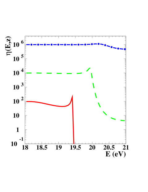
Figure 6: Modification factor [17] from our analytical calculation versus cosmic ray energy. Curves are for different redshifts (top: $z=0.002$; middle: $z=0.02$; bottom $z=0.2$) and assuming no cosmological constant in order to compare results to [17, 7].

In Figure 7 is shown (black solid curve) the cosmic ray expected flux versus energy ($E$) at Earth multiplied by $E^{3}$ from a cosmological injection spectrum with $\alpha=2.6$. The expected GZK feature is present.

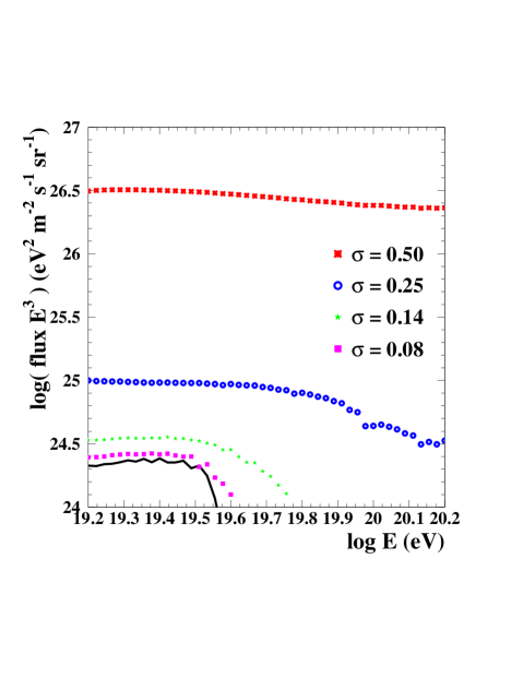
Figure 7: Cosmic ray energy spectrum ($\times E^{3}$) from a cosmological flux (solid black line) with spectral index $\alpha=2.6$. The other curves are the energy spectrum convoluted with a lognormal error with standard deviations $\sigma$ as shown.

3 Errors effects on the energy reconstruction

We will now assume that the cosmic ray energy spectrum from a cosmological isotropic distribution of sources is the true spectrum. To understand how an error in the reconstructed energy affects the spectrum, we convolute the cosmological flux assuming a lognormal error on the energy.

The lognormal distribution is given by

$$\frac{dP(E^{\prime},E)}{d\ln E}=k\exp\left[-\frac{1}{2\sigma^{2}}\log^{2}\frac{E^{\prime}}{E}\right]$$ (5)

where $k=1\,/\,\sqrt{2\pi}\sigma$ is a normalization to unit area and $\sigma$ is the standard deviation of $\log_{10}E$. When a lognormal error in the energy reconstruction is assumed, the flux will be convoluted in the following way:

$$dF^{\prime}(E)=F(E^{\prime})\frac{dP(E^{\prime},E)}{dE}dE^{\prime}$$ (6)

where F is given by Equation 1.

The expected flux ($\times E^{3}$) for energies reconstructed with a lognormal error distribution is shown in Figure 7. The curves are for a spectral index $\alpha=2.6$ and $\sigma=0.08$, 0.14, 0.25 and 0.5 as labeled.

It is very clear that not only the flux increases by a constant factor but also the GZK feature is smeared. As shown in Figures 1 and 2, the standard deviation in the lognormal distribution will be obtained in an ideal case where thousands of events are detected depends on the energy of the primary particle. It is 0.08 for a $10^{20}$ eV proton and 0.14 for a $10^{18}$ eV proton. Figure 7 shows that if the standard deviation is above 0.14 the GZK cutoff will show up at higher energies than in the true spectrum.

4 Results and Conclusions

Figure 7 shows how the energy spectrum from a cosmological flux is smeared due to a lognormal error in the energy reconstruction. Intrinsic shower fluctuations leads to a lognormal distribution of observed energy deposition and number of particles in the shower. A standard deviation of $log_{10}E$ equal to 0.25 is enough to modify not only the shape as well as the normalization of the spectrum measured at the Earth. As a consequence the GZK feature will be smeared and might not be detected at all. Such a $\sigma$ (standard deviation of $\log_{10}E$) can easily result from a detector that only samples a small portion of the total number of particles. This will be more crucial to ground detectors since their particle sample is detected all at one height. The standard deviation of the intrinsic energy error distribution for ground detectors is expected to be larger than for fluorescence detectors.

The air fluorescence detectors will have lower intrinsic lognormal standard deviation as they observe the full development of the shower through the range of view. They miss observing only what goes into the ground or is out of the field of view.

As the Pierre Auger Observatory will not only increase the data sample to a significant level, but also combine both ground and fluorescence techniques, it will have constraints to understand and better control the errors in the energy reconstruction. In this way it is possible to keep the standard deviation of the intrinsic lognormal energy error to its minimum value.

The lognormal curves shown in Figure 1 and 2 have $\sigma=0.08$ and 0.14 respectively. However one can expect a larger value from an observed distribution since the detectors sample only a portion of the total number of particles. On the other hand the standard deviation of the distribution depends on the ground level altitude and therefore an analysis equivalent to ours has to be done for a specific depth.

Figure 8 shows that the lognormal error in the energy is also affected by the spectral index of the injection spectra. However the error in the energy reconstruction will smear the flux in a significant way independently of the spectral index.

Figure 8: Same as Figure 7 but with spectral index $\alpha=3.0$ (top) and $\alpha=2.3$ (bottom). Curve with crosses (x) has $\sigma=0.5$; circles (o), $\sigma=0.25$ and squares, $\sigma=0.1$.

We have shown that a lognormal error in the energy reconstruction of the UHECR spectra will affect not only the shape but also the normalization of the measured energy spectra. A standard deviation equal to or greater than 0.25 will smear the GZK feature. As a consequence this feature will not be seen. This result is independent of the spectral index of the injection spectra.

In conclusion, the establishment of the presence or not of the GZK cutoff in the UHECR spectrum depends not only in a larger data sample but also in the determination of the shape of the energy error distribution. The standard deviation of this distribution has to be kept to its intrinsec value. If it is equal or greater to 0.25 the GZK feature will be smeared and not be detected.

Acknowledgements – We thank Don Groom for useful comments. This work was partially supported by NSF Grant Physics/Polar Programs No. 0071886 and in part by the Director, Office of Energy Research, Office of High Energy and Nuclear Physics, Division of High Energy Physics of the U.S. Department of Energy under Contract Num. DE-AC03-76SF00098 through the Lawrence Berkeley National Laboratory.

References

- [1] K. Greisen, Phys. Rev. Lett. 16, 748 (1966); G. T. Zatsepin and V. A. Kuźmin, Pis’ma Zh. Eksp. 4, 114 (1966) and JETP Lett., 4, 78, 1966).
- [2] D. J. H. Chung, G. F. Farrar and E. W. Kolb, Phys. Rev. D 57, 4606 (1998).
- [3] I. F. M. Albuquerque, G. F. Farrar and E. W. Kolb, Phys. Rev. D 59, 015021 (1999).
- [4] J. W. Elbert and P. Sommers, Astrophys. J. 441, 151 (1995).
- [5] M. Takeda et al., Astropart. Phys. 19, 447 (2003); M. Takeda et al., Phys. Rev. Lett. 81, 1163 (1998).
- [6] R. U. Abbasi et al., astro-ph/0501317 (2005).
- [7] D. de Marco, P. Blasi and A. V. Olinto, Astropart. Phys., 20, 53 (2003).
- [8] T. Stanev, astro-ph/0303123 (2003).
- [9] www.auger.org
- [10] T. Gaisser,“Cosmic Rays and Particle Physics”, Cambridge University Press (1990).
- [11] Pierre Auger Project Design Report; www.auger.org.
- [12] AIRES package (Airshower Extended Simulations v.2.6.0), S. J. Sciutto, astro-ph/0106044; www.fisica.unlp.edu.ar/auger/aires.
- [13] C.O. Escobar, L.G. Santos and R.A. Vazquez, astro-ph/0202172 (2002).
- [14] M. Blanton, P. Blasi and A. V. Olinto, Astropart. Phys. 15, 275 (2001). In this paper it is shown that at ultra high energies an isotropic cosmic ray flux does not differ much from a flux originated from a distribution compatible with the one observed from large scale structure.
- [15] G. Blumenthal, Phys. Rev. D 1, 1596 (1970).
- [16] J. Geddes, T. C. Quinn and R. M. Wald, Astrophys. J., 459, 384 (1996).
- [17] V. S. Berezinsky and S. I. Grigore’va, Astron. Astrophys. 199, 1 (1988).