A simple parameterization of the consequences of deleptonization for simulations of stellar core collapse

Abstract

A simple and computationally efficient parameterization of the deleptonization, the entropy changes, and the neutrino stress is presented for numerical simulations of stellar core collapse. The parameterization of the neutrino physics is based on a bounce profile of the electron fraction as it results from state-of-the-art collapse simulations with multi-group Boltzmann neutrino transport in spherical symmetry. Two additional parameters include an average neutrino escape energy and a neutrino trapping density. The parameterized simulations reproduce the consequences of the delicate neutrino thermalization/diffusion process during the collapse phase and provide a by far more realistic alternative to the adiabatic approximation, which has often been used in the investigation of the emission of gravitational waves, of multidimensional general relativistic effects, of the evolution of magnetic fields, or even of the nucleosynthesis in simulations of core collapse and bounce. For supernova codes that are specifically designed for the postbounce phase, the parameterization builds a convenient bridge between the point where the applicability of a stellar evolution code ends and the point where the postbounce evolution begins.

1. Introduction

Since the mid sixties, the gravitational collapse of stars has been studied based on computer simulations (Colgate & White, 1966; Arnett, 1966). Investigated topics in the collapse phase included general relativistic dynamics (May & White, 1967), magnetic fields (Leblanc & Wilson, 1970), deleptonization and neutrino trapping (Sato, 1975; Mazurek, 1976), progenitor rotation (Müller & Hillebrandt, 1981), dissociation energy (Arnett, 1982), neutrino transport and thermalization (Wilson, 1985; Bruenn, 1985), nuclear electron capture (Bethe et al., 1979; Cooperstein & Wambach, 1984), and the emission of gravitational waves (Moore, 1981), to name only a few of the many possible references. Later, the field has somewhat separated into two rather disjunct lines of research. On the one hand, the increasing computing power was focused on the details of the neutrino physics and neutrino transport in spherical symmetry. On the other hand, the computational resources were invested in multidimensional dynamics for the investigation of rotating progenitors (Ott et al., 2004; Ardeljan et al., 2004), general relativity (Dimmelmeier et al., 2002; Siebel et al., 2003; Shibata & Sekiguchi, 2005; Duez et al., 2005), and magnetic fields (Yamada & Sawai, 2004; Kotake et al., 2004; Liebendörfer et al., 2005). Only few recent multidimensional collapse simulations made the effort to include neutrino physics. These schemes are either very computationally expensive (Buras et al., 2003; Müller et al., 2004; Walder et al., 2005) or rely on simplifications of the neutrino transport and its microphysics (Kotake et al., 2003b; Fryer & Warren, 2004).

Among the neutrino physics that is most difficult to capture are accurate composition-dependent rates of electron captures on nuclei (Langanke et al., 2003) in the early and medium phase of collapse and the competition between neutrino diffusion and neutrino thermalization in the later phase of the collapse (Bruenn, 1985; Myra & Bludman, 1989).

Electrons at high matter density are degenerate so that they are captured with large energies on bound or free protons. The produced high energy neutrinos first thermalize by electron scattering until their energy-dependent mean free path is large enough to make diffusion competitive. As the trapped neutrinos become degenerate themselves in the late stage of collapse, the ability to stream away at low energy actually becomes the bottleneck for further deleptonization. Most recent simulations of this thermalization-diffusion process are based on an individual treatment of different neutrino energy bins with Boltzmann neutrino transport (Mezzacappa & Bruenn, 1993b; Bruenn & Mezzacappa, 1997; Rampp & Janka, 2000; Liebendörfer et al., 2001; Thompson et al., 2003; Hix et al., 2003). The neutrino physics enters the equations of hydrodynamics in the form of three different source terms: as an electron fraction change rate, as an energy or entropy source, and as a source of acceleration by neutrino stress.

This paper aims to bridge the two lines of research by an efficient and very simple prescription of how published and future results of accurate neutrino transport simulations in spherical symmetry could be incorporated in the hydrodynamics of core collapse for a more realistic study of the multidimensional dynamics, the role of magnetic fields, and the emission of gravitational waves than with adiabatic simulations.

A parameterization of the three source terms is individually described and evaluated in $\S$2-4. Additional tests of the robustness of the parameterization with respect to model changes or differences in the dynamics are conducted in $\S$5. After the conclusion, more code-specific details of the implementation are defined in the appendix.

2. Deleptonization

Stellar core collapse proceeds by an imbalance between the self-gravitating forces of the inner core and its fluid pressure. The baryons contribute the most significant part to the gravitational mass of the stellar core while the degenerate electron gas provides the dominant contribution to the pressure. The electron fraction, defined as the number of electrons per baryon in the gas, is therefore the most fundamental quantity for the stability of the inner core and the evolution of its size during the dynamical collapse. The electron fraction evolves by electron captures on nuclei and the emission of the produced electron neutrinos. See (Martínez-Pinedo et al., 2004) for a recent review of the nuclear input physics before and during core collapse. The collapse continues until the matter at the center reaches nuclear density. Strong interactions reduce the compressibility at that point and the inner core bounces. The outgoing pressure wave turns into a shock wave as soon as it reaches the sonic point at the edge of the homologously collapsing inner core. The size of the inner core is important because it determines the location of this transition, the initial energy imparted to the shock, and the amount of matter outside of the shock that will be accreted and dissociated in the ongoing evolution.

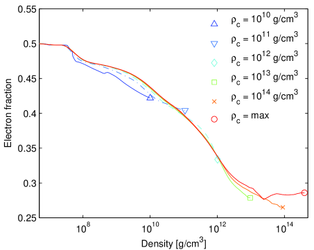
Figure 1.— Electron fraction profiles during core collapse in model G15 (Liebendörfer et al., 2005). Each line shows the electron fraction as a function of density at a given time. The time slices have been chosen to represent each decade in the central density, $\rho_{c}$, as indicated in the legend. The parameterization of the electron fraction, $Y_{e}$, is based on the fact that the profile $Y_{e}\left(\rho\right)$ is only a weak function of time.

Figure 1 shows the electron fraction, $Y^{G15}_{e}\left(\rho,t\right)$, as a function of density, $\rho$, at different times, $t$. The data has been taken from a general relativistic core collapse simulation with Boltzmann neutrino transport and “standard” input physics. The selected time slices correspond to the instances at which the central density reaches $10^{10}$ g/cm³, $10^{11}$ g/cm³, $\ldots$, $10^{14}$ g/cm³, and finally $\rho_{max}$ at bounce. Figure 1 demonstrates that the function $Y_{e}\left(\rho,t\right)$ depends only weakly on time. Hence, it could be interesting to investigate how hydrodynamics simulations behave when the computationally expensive calculation of $Y_{e}\left(\rho,t\right)$ is replaced by linear interpolation in the logarithmic density of a time-independent tabulated template of $\bar{Y}_{e}\left(\rho\right)$. Because the electron fraction profile should be as accurate as possible at the time of bounce, when the final size of the inner core is determined, the choice $\bar{Y}_{e}\left(\rho\right)\equiv Y^{G15}_{e}\left(\rho,t_{b}\right)$ at the time of bounce, $t_{b}$, will be investigated. The data for the bounce electron fraction profile of model G15 are listed in machine-readable tables in (Liebendörfer et al., 2005). Alternatively, a fitting formula is provided here to increase the flexibility of the approach. The fitting of $\bar{Y}_{e}\left(\rho\right)$ is based on a piecewise linear approximation with a piecewise cubic correction. The parameters are two points in the $\rho$-$Y_{e}$ space, $\left(\rho_{i},Y_{i}\right)$, and a scale, $Y_{c}$, of the correction. Suggested values of the parameters are given in Table 1.

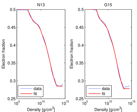
Figure 2.— Comparison of the fit formula for the electron fraction profile at bounce with the original data of models N13 and G15. The agreement is much more accurate than the deviations investigated in Fig. 3. The rise of $Y_{e}$ at the center of the G15 model is not reproduced by the fit. However, no improvement for the simulations would be obtained, because the minimum function in Eq. (2) does not allow electron fraction increases anyway.

Table 1Parameters for the fitting-formula.

	N13			G15
	$\rho_{i}$ [g/cm3]	$Y_{i}$		$\rho_{i}$ [g/cm3]	$Y_{i}$
$i=1$…	$2\times 10^{7}$	$0.5$		$3\times 10^{7}$	$0.5$
$i=2$…	$2\times 10^{13}$	$0.285$		$2\times 10^{13}$	$0.278$
$Y_{c}$…		$0.035$			$0.035$

The fitting formula reads

$$x\left(\rho\right) = \max\left[-1,\min\left(1,\frac{2\log\rho-\log\rho_{2}-\log\rho_{1}}{\log\rho_{2}-\log\rho_{1}}\right)\right]$$

$$Y_{e}\left(x\right) = \frac{1}{2}\left(Y_{2}+Y_{1}\right)+\frac{x}{2}\left(Y_{2}-Y_{1}\right)$$ (1)

$$+ Y_{c}\left[1-|x|+4|x|\left(|x|-1/2\right)\left(|x|-1\right)\right].$$

The comparison of the fit with the original data for models N13 and G15 in Fig. 2 is very satisfactory. Table 1 shows that the fits for the two models only differ in the density at the base of the silicon-oxygen layer, $\rho_{1}$, and in the central electron fraction, $Y_{2}$. The fit can thus easily be modified by variation of these two physical quantities.

The implementation of an electron fraction evolution along $\bar{Y}_{e}\left(\rho\right)$ in a pure hydrodynamics scheme is achieved by the simple prescription

$$\frac{\delta Y_{e}}{\delta t}=\frac{\min\left(0,\bar{Y}_{e}\left(\rho\left(t+\delta t\right)\right)-Y_{e}\left(t\right)\right)}{\delta t},$$ (2)

where the variation is taken at the same fluid element. The minimum function guarantees that the electron fraction monotonically decreases even if transient instances would occur where $\bar{Y}_{e}$ would be larger than the actual $Y_{e}$. At the very start of a simulation, for example, Fig. 1 indicates that $Y_{e}<\bar{Y}_{e}$ almost everywhere ($Y_{e}$ in the progenitor data is represented by the profile belonging to the central density $\rho_{c}=10^{10}$ g/cm³; $\bar{Y}_{e}$ is represented by the profile belonging to $\rho_{c}=max$). Thus, the deleptonization described by Eq. (2) sets in smoothly after a short time of adiabatic compression during which the original electron fraction profile moves to the right in the $\rho$-$Y_{e}$ space shown in Fig. 1 to join the bounce profile, $\bar{Y}_{e}$. The latter is then followed thereafter.

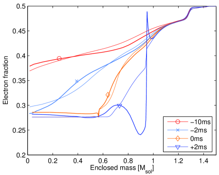
Figure 3.— Electron fraction profiles as functions of enclosed mass at $10$ ms and $2$ ms before bounce, at bounce, and at $2$ ms after bounce. The thick lines represent the accurate evolution of model G15 with Boltzmann neutrino transport. The thin lines represent the solution with the simple parameterization described in Eq. (2). Overall, the deleptonization is in agreement. The differences can be traced back to the earlier time slices where deviations of up to $5\%$ in the deleptonization do occur. The time slice at $2$ ms after bounce illustrates that the simple approximation for the deleptonization breaks down with the launch of the neutrino burst at an enclosed mass $\sim 0.8$ M_⊙.

Figure 3 compares the resulting evolution of the electron fraction to the evolution obtained in the full model G15 with accurate neutrino transport. The small deviations between the two solutions are readily explained with the profiles shown in Fig. 1: At low density, early time slices (marked by triangles) have a lower electron fraction than the bounce profile (marked by a circle). At densities $\sim 10^{11-12}$ g/cm³ the realistic profile (marked by a diamond) assumes a larger electron fraction than the bounce profile. Time slices that reach to even larger densities (marked by a square and a cross) show lower electron fractions than the bounce profile. Because the bounce profile has been taken as template for the parameterization, the same differences are reflected in Fig. 3, most clearly visible in the profile at $2$ ms before bounce. The parameterized deleptonization leads to somewhat higher $Y_{e}$ values in the outer layers, to lower $Y_{e}$ values in intermediate regions, and to higher $Y_{e}$ values near the center. The deviations are within $5\%$.

The $Y_{e}$ value in model G15 rises again around nuclear density because of the increasing neutron degeneracy. Due to the minimum function, this change is not captured by Eq. (2) so that the central $Y_{e}$ value at bounce in the parameterized evolution eventually falls below the corresponding value in the G15 model. A parameterization of the lepton fraction instead of the electron fraction would improve this, because the $Y_{e}$ would then assume its correct equilibrium value after neutrino trapping. Also the entropy changes would more consistently derive from lepton fraction changes than from electron fraction changes. The decision to work with the electron fraction was motivated by the dominant role of $Y_{e}$ in the determination of the Chandrasekhar mass of the bouncing core, because $Y_{e}$ is a common input variable of realistic equations of state, and because a numerical determination of weak equilibrium would be required to find $Y_{e}$ otherwise.

The $Y_{e}$ profile of model G15 at $2$ ms after bounce shows the prominent electron fraction trough that arises when the accretion shock dissociates matter at neutrino-transparent densities around the enclosed mass $\sim 0.9$ M_⊙ . The huge number of neutrinos emitted in the neutrino burst also leads to neutrino absorption ahead of the shock (manifest in the $Y_{e}$ peak at $0.95$ M_⊙ in the time slice at $2$ ms after bounce). These $Y_{e}$-changes can of course not be expected to be represented by Eq. (2) based on the stationary bounce template. More sophisticated techniques are necessary to adequately implement the neutrino physics in the long-term postbounce phase.

3. Entropy changes

The electron captures during collapse are not only changing the electron fraction, the matter entropy is affected as well. The baryons are in nuclear statistical equilibrium and the electrons are in thermal equilibrium. Thus, the increments of the entropy per baryon, $\delta s$, are determined by the values of the chemical potentials $\mu_{n}$, $\mu_{p}$, and $\mu_{e}$ of neutrons, protons, and electrons, respectively. Additionally, there is an energy transfer between matter and neutrinos, $\delta q$ (e.g. (Bruenn, 1985) and references therein),

$$T\delta s=-\delta Y_{e}\left(\mu_{e}-\mu_{n}+\mu_{p}\right)+\delta q.$$ (3)

The temperature of the fluid is denoted by $T$. Depending on the density of the material and the energy of the produced neutrinos, the neutrino can either (i) directly escape, (ii) thermalize and escape, or (iii) be trapped for longer than the dynamical time scale.

In regime (i), $\delta q=\delta Y_{e}\left<E\right>$ where $\left<E\right>$ is the average energy of the freely escaping neutrinos (Bethe, 1990), thus

$$T\delta s=-\delta Y_{e}\left(\mu_{e}-\mu_{n}+\mu_{p}-\left<E\right>\right).$$ (4)

In this regime, electron capture on nuclei dominates over electron capture on protons. Due to the average Q-value of the nuclei $\sim 3$ MeV (Bruenn, 1985) the neutrinos are produced with an average energy that is only marginally larger than $\mu_{e}-\mu_{n}+\mu_{p}$. The corresponding small entropy decrease in this regime shall be neglected in the following parameterization.

In regime (ii) the produced neutrinos start to be trapped by coherent scattering off heavy nuclei. The increasing matter density causes the electron chemical potential to rise so that the neutrinos are produced with higher initial energies. As the neutrino mean free path is proportional to $E_{\nu}^{-2}$, the fastest way of escape proceeds through thermalization at the high end of the neutrino energy spectrum with a transition to diffusion and escape at its low end. Figure 7 in (Martínez-Pinedo et al., 2004) illustrates this thermalization process, which ends with a final escape energy of order $E_{\nu}^{esc}\sim 10$ MeV. For the following parameterization of the entropy changes, $E_{\nu}^{esc}$ is used as a constant parameter that defines where regime (ii) commences, namely when $\mu_{e}-\mu_{n}+\mu_{p}-E_{\nu}^{esc}>0$. The entropy increase is then evaluated according to

$$\frac{\delta s}{\delta t}=-\frac{\delta Y_{e}}{\delta t}\frac{\mu_{e}-\mu_{n}+\mu_{p}-E_{\nu}^{esc}}{T},$$ (5)

where $\delta Y_{e}/\delta t$ is given by Eq. (2).

At even higher densities, in regime (iii), the neutrinos are not able to escape before bounce. They are in equilibrium with the fluid so that $\delta q$ in Eq. (3) is determined by the neutrino chemical potential, $\delta q=\delta Y_{e}\mu_{\nu}$. The neutrinos form a normal gas component without transport abilities and the entropy is conserved in accordance with Eq. (3) and the equilibrium condition $\mu_{e}+\mu_{p}=\mu_{n}+\mu_{\nu}.$ As second parameter, a density threshold $\rho_{trap}\sim 2\times 10^{12}$ g/cm³ is introduced to define the beginning of regime (iii) beyond which no further entropy changes are taken into account.

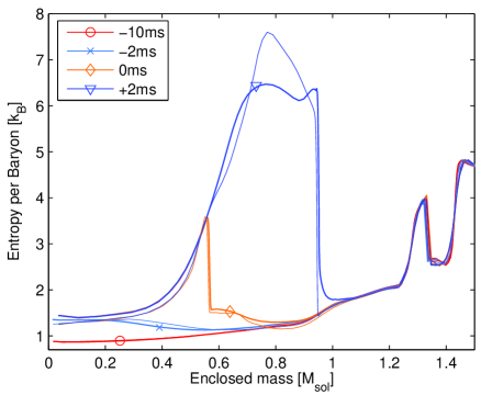
Figure 4.— Profiles of the entropy per baryon as functions of enclosed mass at $10$ ms and $2$ ms before bounce, at bounce, and at $2$ ms after bounce. The thick lines represent the accurate evolution of model G15 with Boltzmann neutrino transport. The thin lines represent the solution with the simple parameterization described in Eq. (5). The entropy evolution is in good agreement during collapse, but drops to about $7\%$ below the reference values after bounce. The time slice at $2$ ms after bounce shows again the prominent difference caused by the neutrino burst. The corresponding energy loss is not captured by the parameterization and leads to an overestimate of the entropy around an enclosed mass $\sim 0.8$ M_⊙.

Figure 4 presents the entropy evolution based on Eq. (5) in comparison to the entropy profiles of model G15 with comprehensive neutrino transport. The two parameters used in Eq. (5) enable nice agreement in the collapse phase (profiles at $10$ ms and $2$ ms before bounce). The density at which the entropy starts to rise is mainly controlled by $E_{\nu}^{esc}=10$ MeV. The level of the central entropy is mainly determined by the choice of $\rho_{trap}=2\times 10^{12}$ g/cm³. The values of the two parameters have not been particularly fine-tuned because they should rather represent a generic estimate than a multi-digit optimum for one particular model. The $\sim 7\%$ lower entropy in the parameterized evolution has no noticeable consequences for the dynamics of the cold matter in the inner core. The entropy profiles at $2$ ms after bounce show the expected differences at late time due to the omission of the neutrino burst in the parameterization. The postshock region in the realistic G15 calculation is significantly cooler because of the energy loss inferred by the neutrino emission. The adjacent region ahead of the accretion shock is somewhat hotter in model G15 due to neutrino absorptions.

4. Neutrino stress

Neutrino stress is the third important quantity at the interface between neutrino transport and hydrodynamics. Although the neutrino pressure only contributes a fraction to the gas pressure, it influences the size of the inner core when the gas pressure and the gravitational forces cancel to a large extent. In regime (iii), i.e. the optically thick region where transport processes can be neglected, the neutrino stress is determined by the gradient of the neutrino pressure

$$\frac{d\mathbf{v}}{dt}=-\frac{\nabla p_{\nu}}{\rho}=-4\pi r^{2}\frac{\partial p_{\nu}}{\partial m},$$ (6)

where $d\mathbf{v}/dt$ is the Lagrangean time derivative of the velocity. The term in the middle is the general expression; the term on the right hand side is its spherically symmetric limit based on an enclosed mass $m(r)$ at radius $r$. All general relativistic effects shall be neglected in the derivation of this simple parameterization. The neutrino pressure, $p_{\nu}$, is readily evaluated based on the thermodynamic state of the fluid,

$$p_{\nu}=\frac{4\pi}{3\left(hc\right)^{3}}\left(kT\right)^{4}F_{3}\left(\frac{\mu_{\nu}}{kT}\right).$$ (7)

The neutrino chemical potential is given by $\mu_{\nu}=\mu_{e}-\mu_{n}+\mu_{p}$. The constants $h$, $c$, and $k$ refer to the Planck constant, the speed of light, and the Boltzmann constant, respectively. $F_{n}\left(\eta\right)=\int_{0}^{\infty}x^{n}\left(e^{x-\eta}+1\right)^{-1}dx$ is the Fermi-Dirac function of order n (Rhodes, 1950).

For an implementation of neutrino stress in the optically thin regime, an estimate of the neutrino number luminosity is needed. It can be derived from the deleptonization in Eq. (2) and the requirement of lepton conservation. The simplest possible approximation in the construction of the neutrino flux from distributed sources is that the neutrinos leave isotropically and without time delay from the locations of deleptonization. Even if this assumption is obviously wrong in core collapse, it leads to a useful first approximation of the non-local flux geometry (Gnedin & Abel, 2001). Firstly, the deleptonization scheme in Eq. (2) already suppresses sources at high opacities. Secondly, lepton conservation requires that an isotropic source contributes with the square of its inverse distance so that closeby sources from this side of the neutrinosphere influence the direction of the neutrino flux more strongly than remote sources from the opposite side. With this assumption, the neutrino number flux can be expressed by the gradient of a scalar field, $\psi$, which fulfills the Poisson equation

$$\Delta\psi=\rho N_{A}\frac{\delta Y_{e}}{\delta t}.$$ (8)

In spherical symmetry, the neutrino number luminosity based on Eq. (8) results in a straightforward integration of all enclosed sources,

$$L(r)=4\pi r^{2}\frac{\partial\psi}{\partial r}=-\int_{0}^{m(r)}\frac{\delta Y_{e}}{\delta t}N_{A}dm.$$ (9)

Avogadro’s number is denoted by $N_{A}$.

Let us stay in the spherically symmetric limit to derive an extension of the neutrino pressure to the optically thin regions. The neutrino stress can be expressed as a convolution of the neutrino number luminosity, the neutrino energy, and the energy-dependent reaction cross sections (Mezzacappa & Bruenn, 1993a). If the reaction cross sections are represented by the inverse mean free path, $\lambda^{-1}\left(E\right)$, one obtains based on the neutrino distribution function, $f\left(E,\mu\right)$,

$$\frac{dv}{dt}=\frac{2\pi}{\left(hc\right)^{3}\rho}\int\frac{1}{\lambda\left(E\right)}f\left(E,\mu\right)E^{3}dE\mu d\mu.$$ (10)

The neutrino momentum phase space element, $E^{2}dEd\mu$, is described by the neutrino energy, $E$ , and the propagation angle cosine, $\mu$, with respect to the radial direction. Let’s now assume that the spectrum of the number luminosity is well approximated by a Fermi-Dirac function with degeneracy parameter $\eta$. The number luminosity can then be expressed as

$$L = 4\pi r^{2}c\frac{2\pi}{\left(hc\right)^{3}}\int f\left(E,\mu\right)E^{2}dE\mu d\mu$$ (11)

$$\simeq 4\pi r^{2}c\frac{2\pi}{\left(hc\right)^{3}}\left(kT_{\nu}\right)^{3}F_{2}\left(\eta\right)H.$$

For the following rough estimate of the decline of the neutrino stress in the outer layers, it is further assumed that the mean free path scales as $\lambda^{-1}\propto\rho E^{2}$, so that the energy integration in Eq. (10) can be evaluated and expressed by the number luminosity in Eq. (11),

$$\frac{dv}{dt}\propto\left(kT_{\nu}\right)^{6}F_{5}\left(\eta\right)H\propto\left(kT_{\nu}\right)^{3}\frac{F_{5}\left(\eta\right)}{F_{2}\left(\eta\right)}\frac{L}{4\pi r^{2}}.$$ (12)

The neutrino temperature, $kT_{\nu}$, and the degeneracy parameter, $\eta$, cannot easily be derived as a function of radius without solving a more detailed transport problem. Though, at high opacity, they limit to the matter temperature, $kT$, and the neutrino degeneracy, $\mu_{\nu}/kT$, respectively.

The neutrino stress for the hydrodynamics simulation is now generated by the following procedure: An estimate for the number luminosity is given by Eq. (9). Then, at all densities larger than a specified neutrino trapping density $\rho_{trap}$, the neutrino stress is evaluated according to Eqs. (6) and (7). With the neutrino stress at density $\rho_{trap}$, a constant $C$ is defined that attaches the scaling estimate found in Eq. (12) to the neutrino stress given by Eq. (6),

$$C=-4\pi r^{2}\frac{\partial p_{\nu}}{\partial m}\left[\left(kT\right)^{3}\frac{F_{5}\left(\mu_{\nu}/kT\right)}{F_{2}\left(\mu_{\nu}/kT\right)}\frac{L}{4\pi r^{2}}\right]^{-1}.$$ (13)

In Eq. (13), $r$, $\partial p_{\nu}/\partial m$, $T$, $\mu_{\nu}$, and $L$ are evaluated at the transition density $\rho_{trap}$. Now, before Eq. (12) can be applied to extend the neutrino stress to the region $\rho<\rho_{trap}$, approximations for $kT_{\nu}$ and $\eta$ must be found for regime (i). There, it is assumed that the neutrino spectrum is well represented based on a degeneracy $\eta=0$. It is then consistent with $\S$3 and the assumption of spherical symmetry if I express the neutrino temperature by the average neutrino energy parameter, $E_{\nu}^{esc}$, and set $kT_{\nu}=F_{2}\left(0\right)/F_{3}\left(0\right)E_{\nu}^{esc}$. The simplest continuous transition of the neutrino stress from regime (iii) to regime (i) is realized by the adoption of the larger of the two limiting cases in each intermediate point. Hence, at $\rho<\rho_{trap}$, the neutrino stress is approximated by

$$\frac{dv}{dt}=\frac{CL}{4\pi r^{2}}\max\left[\left(kT\right)^{3}\frac{F_{5}\left(\frac{\mu_{\nu}}{kT}\right)}{F_{2}\left(\frac{\mu_{\nu}}{kT}\right)},\left(E_{\nu}^{esc}\right)^{3}\frac{F_{2}^{2}\left(0\right)F_{5}\left(0\right)}{F_{3}^{3}\left(0\right)}\right],$$ (14)

where $r$, $T$, $\mu_{\nu}\equiv\mu_{e}-\mu_{n}+\mu_{p}$, and the estimate of $L$ according to Eq. (9) represent the local values at the point where $dv/dt$ is evaluated. Suggestions with respect to the implementation of this spherically symmetric neutrino stress in a multidimensional hydrodynamics code and convenient approximations for the evaluation of the Fermi integrals are collected in the appendix.

This procedure circumvents any explicit reference to cross sections and is therefore simple to apply. Of course, the cross sections do enter the constant $C$ implicitly via the relation between the neutrino pressure gradient and the number luminosity at the transition density $\rho_{trap}$. As the value of the number luminosity is derived from Eq. (2), it reflects the deleptonization rate in the reference calculation with full transport which is based on information about the opacities used in the run that produced the electron fraction template at bounce time.

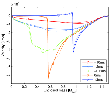
Figure 5.— Velocity profiles as functions of enclosed mass at $10$ ms, $2$ ms, and $0.2$ ms before bounce, at bounce, and at $2$ ms after bounce. The thick lines represent the accurate evolution of model G15 with Boltzmann neutrino transport. The thin lines represent the solution with the simple parameterization described in Eqs. (6) and (14). The homologous infall is in nice agreement initially. The time slice at $2$ ms before bounce shows a soft outgoing pressure wave that is mainly caused by electron fraction differences near the center. It causes perturbations around an enclosed mass of $0.6$ M_⊙ in the $-0.2$ ms time slice. Otherwise, the strong pressure wave from bounce is in good agreement with the reference simulation at that time. The point of shock formation is very similar in both cases. The velocity profiles even continue to coincide some time beyond the emission of the neutrino burst as shown in the time slice at $2$ ms after bounce.

Figure (5) shows a summary of the evolution of velocity profiles. It demonstrates that the collapse dynamics is accurately reproduced with the parameterized neutrino physics. Some differences can still be made out: As discussed in $\S$2, Eq. (2) implies a transient halt in the deleptonization until the density has increased enough that the initial $Y_{e}$ profile (labeled by $\rho_{c}=10^{10}$ in Fig. 1) catches up with the template (labeled by $\rho_{c}=max$). This leads to a small delay in the infall of the outer layers with respect to the reference G15 model. This is visible in the velocity profiles at the enclosed mass of $1$ - $1.2$ M_⊙.

The time slice at $2$ ms before bounce shows a soft outgoing pressure wave in the solution with the parameterized neutrino physics that is not present in the reference model. The first suspicion was that it is related to the treatment of the neutrino stress because its appearance coincides to some extent with the moment when the density $\rho_{trap}$ is reached at the center, i.e. the moment when the applied neutrino stress jumps from zero to the value described by Eq. (14). However, a more careful investigation showed that the dominant reason is the shallower electron fraction profile close to the center in the $-2$ ms time slice (see Fig. 3). The outgoing wave is caused by a combination of the excess electron pressure at the center with the electron pressure deficit around an enclosed mass of $0.4$ M_⊙. It introduces visible perturbations in the vicinity of the position of shock formation in the time slice at $0.2$ ms before bounce. Nevertheless, the much stronger outgoing pressure wave from bounce and its steepening to the bounce-shock are nicely reproduced in the $-0.2$ ms and $0$ ms time slices.

The significant differences induced by the neutrino burst in the electron fraction and entropy profiles at $2$ ms after bounce seem to have surprisingly little influence on the early dynamics. The velocity profiles as functions of enclosed mass still agree at $2$ ms after bounce. The differences in the state of the postshock matter rather affect the shock radius than the shock mass. While the shock in the G15 model is positioned at a radius of $55$ km, it already has reached $63$ km in the parameterized run due to the omission of the lepton and energy loss by the neutrino burst.

5. Model dependence

After the demonstration that this simple parameterization works well for the one model G15, this section aims to explore to what extent the approximations are robust against variations in the dynamics or the initial conditions. A first test is the application of the same parameterization with the same parameters for $E_{\nu}^{esc}$ and $\rho_{trap}$ to a different stellar model. The G15 model discussed above is launched from the (Woosley & Weaver, 1995) model s15s7b2. It has a quite typical iron core $\sim 1.3$ M_⊙. The run N13 in (Liebendörfer et al., 2005) is based on the progenitor of (Nomoto & Hashimoto, 1988) with an especially small iron core $\sim 1.17$ M${}_{\odot}.$

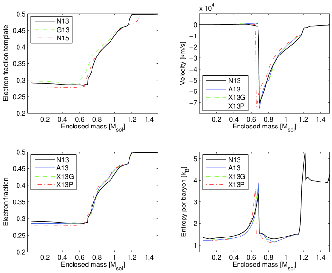
Figure 6.— Profiles at the time of bounce are shown to investigate the dependence of the parameterization on model variations. (a) Electron fraction templates for the N13, G13, and N15 model determined in simulations with full neutrino transport. (b-d) Velocity, electron fraction, and entropy profiles, respectively, for the parameterized simulations at bounce. The label N13 indicates the reference results with neutrino transport. The parameterized simulations A13, X13G, and X13P differ only by the $Y_{e}$-template that has been used. Template N13 has been used for run A13, G13 has been used for run X13G, and N15 has been used for run X13P. Swapping templates between Newtonian and general relativistic simulations introduced no significant differences, while a swapping of templates between progenitors lead to slightly different positions of the shock formation that correlate with the minimum $Y_{e}$ reached in the inner core.

Figure 6 compares different runs at the time of core-bounce. Figure 6a shows the bounce profile $\bar{Y}_{e}\left(\rho\right)=Y^{N13}_{e}\left(\rho,t_{b}\right)$ of the N13 run that was used to specify the deleptonization according to Eq. (2) for the parameterized run A13. The bounce profiles of the N13 and A13 runs are displayed in Fig. 6b-d. The quality of the approximation is very similar to the one discussed above for the G15 model. The same choice of the parameters $E_{\nu}^{esc}$ and $\rho_{trap}$ seems to fit also other stellar models.

The dynamics in the N13 and G15 models is also different. The former has been calculated with Newtonian hydrodynamics and $O(v/c)$ neutrino transport, the latter with general relativistic dynamics and transport. As a second test I investigate how the parameterized solution reacts if the bounce template for a Newtonian simulation is taken from a general relativistic model of the same progenitor model. Thus, a bounce-template G13 in Fig. 6a has been produced from a general relativistic calculation with neutrino transport. A repetition of run A13 with the exchanged template, $\bar{Y}_{e}\left(\rho\right)=Y^{G13}_{e}\left(\rho,t_{b}\right)$ instead of $\bar{Y}_{e}\left(\rho\right)=Y^{N13}_{e}\left(\rho,t_{b}\right)$, leads to the results labeled by X13G in Fig. 6b-d. In spite of the significant dynamical differences in the runs that produced the templates N13 (solid line) and G13 (dashed line) in Fig. 6a, the differences in velocity, electron fraction, and entropy profiles between runs A13 and X13G are barely visible. This means that the template for the parameterization of the microphysics can be extracted from a run whose dynamics differs from the run in which the parameterization will be applied.

A third test has been performed by the exchange of bounce templates between the progenitor models. First, a new template has been created with a Newtonian simulation of the s15s7b2 progenitor model labeled by N15 in Fig. 6. The parameterized Newtonian run X13P has then been launched from the $13$ M_⊙ progenitor model using this $\bar{Y}_{e}\left(\rho\right)=Y^{N15}_{e}\left(\rho,t_{b}\right)$ template. Figure 6b-d shows a small deviation $\sim 6\%$ in the location of the shock formation. Although a given template from one progenitor still seems to be useful for many dynamical investigations that are launched from different progenitor models, it might be recommended to use a template that is derived from the same progenitor to achieve the best accuracy. A closer inspection of the differences reveals the well-known fact that the final deleptonization in the inner core is essential for the location of the shock formation. Because the parameterization in Eq. (2) does not support electron fraction increases, it is the minimum $Y_{e}$ that counts. The minimum $Y_{e}$ in the templates of the N13 and G13 models in Fig. 6a coincide, while $Y_{e}$ in the N15 run reached slightly lower values.

6. Limitations

The described parameterization has been designed to provide a very efficient and reasonably accurate way to lead a hydrodynamics simulation from the onset of collapse of the supernova progenitor star to bounce. It has also been shown to be accurate for the initial rebound of the stellar core. However, the simplicity of the described approach entails several limitations.

The signal of gravitational waves is not likely to be limited to the short time interval around bounce that has traditionally been investigated (Ott et al. (2004) and references therein). In delayed, and especially in neutrino-driven explosions, the signal may decay after the first peak around bounce only to regain strength on a longer time scale of several hundreds of milliseconds, when fluid instabilities in the hot shocked matter between the protoneutron star and the shock front grow to asymmetries on larger scales (Thompson, 2000; Scheck et al., 2004; Müller et al., 2004). The dynamics and the input physics for the description of the cold matter in the collapse phase are fundamentally different from the physics in the hydrostatic, but turbulent, hot mantle of the protoneutron star, which eventually determines the supernova explosion after core-bounce. The suggested scheme has not been designed for the postbounce phase and does not describe any of the weak interaction physics relevant after bounce.

Firstly, the scheme handles only deleptonization and not neutrino transport. No attempt has been made to describe the very delicate neutrino energy deposition behind the stalled accretion shock. Neutrino heating at $50$ ms after bounce and beyond is thought to drive important fluid instabilities. Secondly, the scheme is only applicable to situations where the deleptonization is caused by compression of cold matter. Even if the deleptonization in the condensing accreting material continues to be captured after bounce, major contributions from the emission of the neutrino burst at $2$ ms after bounce and from neutrino diffusion in the dense core are missed by the simple parameterization.

Therefore, if one extends an otherwise adiabatic code with the suggested parameterization for a simulation of the postbounce phase, one obtains the benefit that simulations pass through a significantly more realistic configuration at bounce and that overly fast prompt explosions for small progenitors are avoided. But no improvement is obtained toward an adequate description of the important neutrino physics in the postbounce phase.

Another question is the reliability of the scheme in the collapse phase when fast rotation rates are applied. The density distribution is then significantly less spherically symmetric. I think one can be somewhat optimistic because the parameterization of the deleptonization during collapse in Eqs. (2) and (5) relies more on the local density evolution than on the global geometry. This is supported by the low sensitivity of the parameterization to global dynamical changes investigated in $\S$5. A global asymmetry changes rather the spatial distribution of local conditions than the quality of the local conditions themselves. Relevant local conditions are: the time scale of compression, the density gradient, or the curvature of the isodensity surface at the point of investigation (as a measure of the deleptonizing volume per surface area). These quantities as function of the density may change by several percent with respect to a spherically symmetric scenario, but probabely not by orders of magnitude. If this speculation is true, the parameterization would still be approximately applicable. It is likely that accuracy is lost with increasing asphericity, but the improvement with respect to adiabatic simulations could still be significant.

It would now be tempting to make also the treatment of the neutrino stress multidimensional. Equation (6) already has a multidimensional form and Eq. (14) is readily generalized to

$$\frac{d\mathbf{v}}{dt}=C\nabla\psi\max\left[\left(kT\right)^{3}\frac{F_{5}\left(\frac{\mu_{\nu}}{kT}\right)}{F_{2}\left(\frac{\mu_{\nu}}{kT}\right)},\left(E_{\nu}^{esc}\right)^{3}\frac{F_{2}^{2}\left(0\right)F_{5}\left(0\right)}{F_{3}^{3}\left(0\right)}\right],$$ (15)

where $\psi$ is determined by Eq. (8). Unfortunately, it is not clear, how $C$ should be chosen in the multidimensional setting. Simple choices may imply discontinuities in the transition of the neutrino stress from Eq. (6) to Eq. (15) that could introduce undesired artefacts in the velocity field.

The spherically symmetric implementation of the neutrino stress, as layed out in the appendix, is very simple and physically well-defined, but fails to represent any asymmetries in the shape or temperature of the neutrinospheres and in the emitted neutrino luminosities. This might still be an acceptable limitation because the influence of the neutrino stress (momentum deposition) on the collapse dynamics is not as crucial as the much discussed neutrino heating (energy deposition) later in the postbounce phase. In the postbounce phase, which is not in the scope of this parameterization, asymmetries in the neutrino field can have a significant impact on the dynamics of the shock revival (Kotake et al., 2003a). On the other hand, stellar evolution models point to rather slowly rotating inner cores (Heger et al., 2005; Hirschi et al., 2004) and corresponding collapse simulations with multidimensional neutrino transport have not shown evidence for sizable asymmetries in the neutrino field (Walder et al., 2005).

7. Conclusion

The dynamics of core collapse is dominated by electron pressure. Dynamical simulations are only realistic if they can take account of electron captures on bound or free protons during infall. At increasing densities the electron captures get inhibited by neutrino phase space blocking so that the ability to thermalize and emit the produced neutrinos significantly contributes to the determination of the final electron fraction in the inner core. The lower the electron fraction, the smaller is the mass of the core that bounces when nuclear densities are reached and the smaller is also the initial energy imparted to the outgoing shock. These well-known relationships ask for a careful inclusion of neutrino physics in simulations of stellar core collapse. The most accurate treatment of neutrino transport has been developed in spherical symmetry (Mezzacappa & Messer, 1999; Rampp & Janka, 2002; Thompson et al., 2003; Liebendörfer et al., 2004; Sumiyoshi et al., 2005) where it has been coupled to the most recent evaluation of electron capture rates on heavy nuclei (Langanke et al., 2003; Hix et al., 2003; Marek et al., 2005).

The previous sections present an embarassingly simple and computationally efficient parameterization of the deleptonization in the collapse phase so that the consequences of past and future improvements of the neutrino physics should be straightforward to incorporate in multidimensional simulations that focus on other aspects of core collapse. The scheme is based on electron fraction profiles as function of density at bounce, $\bar{Y}_{e}\left(\rho\right)$, that have been produced by spherically symmetric simulations with full neutrino transport. A fitting formula is provided to conveniently represent these electron fraction profiles and to allow for adjustments to future developments. It is found that the time-evolution of the electron fraction in the simulations, $Y_{e}\left(\rho,t\right)$, follows in reasonable approximation the profile $\bar{Y}_{e}\left(\rho\right)$. The corresponding parameterization brings the electron fraction at bounce, when it is most important for the shock dynamics, very close to the value in the original simulation. Unfortunately, it is not exactly equal because small differences in the time-dependence of the deleptonization will lead to density differences at bounce so that $\bar{Y}_{e}\left(\rho\right)$ is not evaluated at exactly the same position as in the original simulation.

Once the deleptonization is given, the entropy changes and neutrino stress are estimated based on two additional parameters, an average neutrino escape energy, $E_{\nu}^{esc}=10$ MeV, and a neutrino trapping density, $\rho_{trap}=2\times 10^{12}$ g/cm³. These parameters have not been fine-tuned, but may require adaption if the weak interaction physics is changed.

In a comparison of the parameterized runs with the original ones it is found that the dynamics of core collapse is quite accurately reproduced. The parameterized neutrino physics presents a significant improvement with respect to adiabatic treatments. Its accuracy may even rival with neutrino transport approximations that neglect neutrino-electron scattering.

However, some clearly visible inaccuracies do develop. The deleptonization of central zones at high densities proceeds slower than in the reference simulation. This leads to a weak outgoing pressure wave before bounce-density is reached. It propagates to the point of shock formation where it causes moderate perturbations. Inaccuracies due to a deviation in the timing of the deleptonization are also found in the hydrodynamic structure ahead of the shock. These deviations are a direct consequence of the differences between the function $\bar{Y}_{e}\left(\rho\right)$ and the time evolution of the electron fraction in the reference simulation.

The evolution of the electron fraction and entropy is based on the local thermodynamic state of the fluid. This should allow an application also in models where the dynamics moderately differs from the spherically symmetric case with which the electron fraction template has been produced. The less important neutrino stress has been approximated in a spherically averaged manner. An extension to handle asymmetries in the neutrino stress has been sketched, but its accuracy in models with essentially aspherical density distributions remains to be investigated. The sensitivity of the parameterized runs to changes in the model has been tested in two experiments that are accessible with comprehensive neutrino transport: Firstly, a template produced with general relativistic dynamics has been used in a parameterized run with Newtonian gravity and, secondly, a template produced with a 15 $M_{\odot}$ progenitor star has been used in a parameterized run launched from a 13 $M_{\odot}$ progenitor star with a very different structure of the iron core.

It was found that the parameterization is not sensitive to the dynamical differences between general relativistic and Newtonian gravity. The choice of the progenitor for the template, however, has a small influence on the parameterization. The extent of the deviation is directly determined by the difference between the central $Y_{e}$ values in the templates. In the investigated case, the $Y_{e}$ difference translates to $\sim 6\%$ difference in the point of shock formation. I thus believe that one and the same template can be used with different progenitors for qualitative studies of the dynamics. But a progenitor-specific template is recommended for more quantitative investigations.

The parameterization has been designed for the collapse phase and not for the postbounce evolution. It does not contain any physics related to neutrino heating. During collapse, it relies on the weak interaction physics used for the production of the bounce template. The nuclear and weak interaction physics during collapse is an interesting field of research. Progress in its adoption in spherically symmetric simulations has been made (Langanke et al., 2003; Hix et al., 2003) and is likely to continue. Hopefully, this paper enables the efficient transfer of results from state-of-the-art neutrino transport simulations in spherical symmetry to simulations with more spatial degrees of freedom, where the implementation of comprehensive weak interaction physics together with the accurate solution of the energy-dependent multidimensional Boltzmann equation is yet computationally prohibitive.

Appendix A Implementation Details

The simulations with the parameterized neutrino physics are based on the same spherically symmetric general relativistic hydrodynamics code AGILE that was used to solve the equations of hydrodynamics in the original production of the electron fraction templates (Liebendörfer et al., 2005). The interaction between neutrino physics and hydrodynamics proceeds through additional source terms in the conservation equations, i.e. $Y_{e}^{ext}$, $e^{ext}$, and $S^{ext}$ in (Liebendörfer et al., 2002) for electron fraction change rates, total energy change rates, and momentum change rates, respectively. The simulations use the realistic Lattimer-Swesty equation of state version 2.7 (Lattimer & Swesty, 1991). Note that this version is likely to crash whenever one tries to enter the nuclear regime (eosflag=2) with a saved guess of the proton fraction obtained from the dissociated regime (eosflag=3). As convergence in the dissociated regime is robust, it is advisable to save guesses only when they are returned with eosflag=2. In the parameterized runs with AGILE, Eq. (2) is used to set $Y_{e}^{ext}$. The heating rate $e^{ext}$ is found by numerical iteration of the equation of state until the entropy change rate specified by Eq. (5) is realized. The parameter $E_{\nu}^{esc}$ is set to $10$ MeV. Note that the approximation $\delta s/\delta t=0$ in the region where $\mu_{e}-\mu_{n}+\mu_{p}-E_{\nu}^{esc}<0$ will still produce a rate $e^{ext}\neq 0$ when the electron fraction changes. At densities larger than $\rho_{trap}=2\times 10^{12}$ g/cm³, the spherically symmetric limit of Eq. (6) is used to calculate the neutrino stress $S^{ext}$, while at lower densities, Eq. (14) is used. In the general relativistic simulations, the gravitational effect of neutrino energy and pressure has only been taken into account at densities $\rho>\rho_{trap}$. The neutrino pressure is evaluated by Eq. (7) and the specific neutrino energy is set to $e_{\nu}=3p_{\nu}/\rho$. The gravitational effect of the neutrino luminosity was neglected.

All time derivatives, $d/dt$, in Eqs. (2,9,5,6,10,12,14,15) are Lagrangean, i.e. taken at the same mass element. Most hydrodynamics codes are discretized in space and not in mass; they rely on Eulerian time derivatives, $\partial/\partial t$. For the implementation of above equations in these schemes I suggest to use operator splitting. For example, the conservation equations of hydrodynamics should be straightforward to extend with a conservation equation for electron number,

$$\frac{\partial}{\partial t}\left(\rho Y_{e}\right)+\nabla\cdot\left(\mathbf{v}\rho Y_{e}\right)=0.$$ (A1)

In this first step, the electron fraction at location $\mathbf{x}$ is updated from $Y_{e}\left(\mathbf{x},t\right)$ to an intermediate value $Y_{e}^{*}\left(\mathbf{x},t+\delta t\right)$ by the advection of electrons. The electron fraction update is completed in a second step by application of Eq. (2),

$$\frac{\delta Y_{e}}{\delta t}\equiv\frac{Y_{e}\left(\mathbf{x},t+\delta t\right)-Y_{e}^{*}\left(\mathbf{x},t+\delta t\right)}{\delta t}=\frac{\min\left(0,\bar{Y}_{e}\left(\rho\left(\mathbf{x},t+\delta t\right)\right)-Y_{e}^{*}\left(\mathbf{x},t+\delta t\right)\right)}{\delta t}.$$ (A2)

The entropy update can similarily be split into an entropy conserving hydrodynamics update (in whatever form it is realized in the hydrodynamics code) and a Lagrangean change of the specific entropy. For the latter, $\delta Y_{e}/\delta t$ in Eq. (5) is substituted by the result of Eq. (A2).

It is numerically stable to apply the neutrino stress in an operator split fashion as well because the neutrino pressure contributes only of order $10\%$ to the total pressure. The simple spherical limit in Eq. (6) is adequate if the deviations from spherical symmetry are small; the multidimensional form is advised otherwise. The extension of the neutrino stress to the optically thin regime is less straightforward because its derivation was based on some arguments that apply only in spherical symmetry. Eq. (13), for example, extracts the opacities from the spherically symmetric run that produced the electron fraction templates. As long as the asphericity in the density distribution does not exceed half a density scale height, I recommend to use spherically averaged conditions of the multidimensional configuration to evaluate the neutrino stress. The integration of the density over spheres results in an enclosed mass as function of the radius. The integration of the deleptonization in Eq. (A2) over spheres leads to a luminosity estimate according to Eq. (9). Based on the spherically integrated density, energy density, and electron density the equation of state delivers the thermodynamic conditions used in Eq. (14) to derive the neutrino stress for spheres with densities $\rho<\rho_{trap}$. The applicability of the multidimensional Eqs. (8) and (15) in highly asymmetric situations was not numerically investigated because their assessment would require the corresponding reference simulations with multidimensional neutrino transport. In any case, it is important to abandon the application of the neutrino stress in optically thin regions after bounce before the shock reaches the density $\rho_{trap}$ in order to prevent the growth of the constant $C$ in Eq. (13) beyond limits.

The Fermi integrals in $\S$4 are required for degeneracy $\eta\geq 0$. Convenient approximations to $F_{2}\left(\eta\right)$ and $F_{3}\left(\eta\right)$ have been taken from (Epstein & Pethick, 1981), while $F_{5}\left(\eta\right)$ has been derived along similar lines based on (Rhodes, 1950):

$$F_{2}\left(\eta\right) \simeq \frac{1}{3}\left(\eta^{3}+\pi^{2}\eta\right)+\frac{3}{2}\zeta\left(3\right)e^{-\alpha\eta}$$

$$F_{3}\left(\eta\right) \simeq \frac{1}{4}\left(\eta^{4}+2\pi^{2}\eta^{2}+\frac{7\pi^{4}}{15}\right)-\frac{7\pi^{4}}{120}e^{-\eta}$$

$$F_{5}\left(\eta\right) \simeq \frac{1}{6}\left(\eta^{6}+5\pi^{2}\eta^{4}+7\pi^{4}\eta^{2}+\frac{31\pi^{6}}{21}\right)-\frac{31\pi^{6}}{252}e^{-\eta}$$ (A3)

with $\zeta\left(3\right)\simeq 1.202$ and $\alpha=2\pi^{2}/\left(9\zeta\left(3\right)\right)-1\simeq 0.825$.

References

- Ardeljan et al. (2004) Ardeljan, N. V., Bisnovatyi-Kogan, G. S., Kosmachevskii, K. V., & Moiseenko, S. G., 2004, Astrophysics, 47, 37
- Arnett (1966) Arnett, W. D., 1966, Canadian Journal of Physics, 44, 2553
- Arnett (1982) —, 1982, ApJ, 263, L55
- Bethe (1990) Bethe, H. A., 1990, Rev. Mod. Phys., 62, 801
- Bethe et al. (1979) Bethe, H. A., Brown, G. E., Applegate, J., & Lattimer, J. M., 1979, Nucl. Phys. A, 324, 487
- Bruenn (1985) Bruenn, S. W., 1985, ApJS, 58, 771
- Bruenn & Mezzacappa (1997) Bruenn, S. W., & Mezzacappa, A., 1997, Phys. Rev. D, 56, 7529
- Buras et al. (2003) Buras, R., Rampp, M., Janka, H.-T., & Kifonidis, K., 2003, Phys. Rev. Lett., 90, 241101
- Colgate & White (1966) Colgate, S. A., & White, R. H., 1966, ApJ, 143, 626
- Cooperstein & Wambach (1984) Cooperstein, J., & Wambach, J., 1984, Nucl. Phys. A, 420, 591
- Dimmelmeier et al. (2002) Dimmelmeier, H., Font, J. A., & Müller, E., 2002, A&A, 393, 523
- Duez et al. (2005) Duez, M. D., Liu, Y. T., Shapiro, S. L., & Stephens, B. C., 2005, submitted to Phys. Rev. D, astro-ph/0503420
- Epstein & Pethick (1981) Epstein, R. I., & Pethick, C. J., 1981, ApJ, 243, 1003
- Fryer & Warren (2004) Fryer, C. L., & Warren, M. S., 2004, ApJ, 601, 391
- Gnedin & Abel (2001) Gnedin, N. Y., & Abel, T., 2001, New Astronomy, 6, 437
- Heger et al. (2005) Heger, A., Woosley, S. E., & Spruit, H. C., 2005, ApJ, 626, 350
- Hirschi et al. (2004) Hirschi, R., Meynet, G., & Maeder, A., 2004, A&A, 425, 649
- Hix et al. (2003) Hix, W. R., Messer, O. E. B., Mezzacappa, A., Liebendörfer, M., Sampaio, J., Langanke, K., Dean, D. J., & Martínez-Pinedo, G., 2003, Phys. Rev. Lett., 91, 201102
- Kotake et al. (2003a) Kotake, K., Yamada, S., & Sato, K., 2003a, ApJ, 595, 304
- Kotake et al. (2003b) —, 2003b, Phys. Rev. D, 68, 044023
- Kotake et al. (2004) Kotake, K., Yamada, S., Sato, K., Sumiyoshi, K., Ono, H., & Suzuki, H., 2004, Phys. Rev. D, 69, 124004
- Langanke et al. (2003) Langanke, K., Martínez-Pinedo, G., Messer, O. E. B., Sampaio, J. M., Dean, D. J., Hix, W. R., Mezzacappa, A., Liebendörfer, M., Janka, H.-T., & Rampp, M., 2003, Phys. Rev. Lett., 90, 241102
- Lattimer & Swesty (1991) Lattimer, J. M., & Swesty, F. D., 1991, Nucl. Phys. A, 535, 331
- Leblanc & Wilson (1970) Leblanc, J. M., & Wilson, J. R., 1970, ApJ, 161, 541
- Liebendörfer et al. (2004) Liebendörfer, M., Messer, O. E. B., Mezzacappa, A., Bruenn, S. W., Cardall, C. Y., & Thielemann, F.-K., 2004, ApJS, 150, 263
- Liebendörfer et al. (2005) Liebendörfer, M., Rampp, M., Janka, H.-T., & Mezzacappa, A., 2005, ApJ, 620, 840
- Liebendörfer et al. (2002) Liebendörfer, M., Rosswog, S., & Thielemann, F., 2002, ApJS, 141, 229
- Liebendörfer et al. (2001) Liebendörfer, M., Mezzacappa, A., Thielemann, F.-K., Messer, O. E. B., Hix, W. R., & Bruenn, S. W., 2001, Phys. Rev. D, 63, 103004
- Liebendörfer et al. (2005) Liebendörfer, M., Pen, U., & Thompson, C., 2005, Nucl. Phys. A, 758, 59
- Müller et al. (2004) Müller, E., Rampp, M., Buras, R., Janka, H.-T., & Shoemaker, D. H., 2004, ApJ, 603, 221
- Marek et al. (2005) Marek, A., Janka, H. ., Buras, R., Liebendörfer, M., & Rampp, M., 2005, to be published in A&A, astro-ph/0504291
- Martínez-Pinedo et al. (2004) Martínez-Pinedo, G., Liebendörfer, M., & Frekers, D., 2004, submitted to Nucl. Phys. A, astro-ph/0412091
- May & White (1967) May, M. M., & White, R. H., 1967, Comput. Phys., 7, 219
- Mazurek (1976) Mazurek, T. J., 1976, ApJ, 207, L87
- Mezzacappa & Bruenn (1993a) Mezzacappa, A., & Bruenn, S. W., 1993a, ApJ, 405, 669
- Mezzacappa & Bruenn (1993b) —, 1993b, ApJ, 410, 740
- Mezzacappa & Messer (1999) Mezzacappa, A., & Messer, O. E. B., 1999, J. Comput. Appl. Math., 109, 281
- Moore (1981) Moore, T. A., 1981, Ph.D. Thesis
- Müller & Hillebrandt (1981) Müller, E., & Hillebrandt, W., 1981, A&A, 103, 358
- Myra & Bludman (1989) Myra, E. S., & Bludman, S. A., 1989, ApJ, 340, 384
- Nomoto & Hashimoto (1988) Nomoto, K., & Hashimoto, M., 1988, Phys. Rep., 163, 13
- Ott et al. (2004) Ott, C. D., Burrows, A., Livne, E., & Walder, R., 2004, ApJ, 600, 834
- Rampp & Janka (2000) Rampp, M., & Janka, H.-T., 2000, ApJ, 539, L33
- Rampp & Janka (2002) —, 2002, A&A, 396, 361
- Rhodes (1950) Rhodes, P., 1950, Proc. Royal Soc. A, 204, 396
- Sato (1975) Sato, K., 1975, Prog. Theor. Phys., 54, 1325
- Scheck et al. (2004) Scheck, L., Plewa, T., Janka, H.-T., Kifonidis, K., & Müller, E., 2004, Physical Review Letters, 92, 011103
- Shibata & Sekiguchi (2005) Shibata, M., & Sekiguchi, Y., 2005, Phys. Rev. D, 71, 024014
- Siebel et al. (2003) Siebel, F., Font, J. A., Müller, E., & Papadopoulos, P., 2003, Phys. Rev. D, 67, 124018
- Sumiyoshi et al. (2005) Sumiyoshi, K., Yamada, S., Suzuki, H., Shen, H., Chiba, S., & Toki, H., 2005, to be published in ApJ, astro-ph/0506620
- Thompson (2000) Thompson, C., 2000, ApJ, 534, 915
- Thompson et al. (2003) Thompson, T. A., Burrows, A., & Pinto, P. A., 2003, ApJ, 592, 434
- Walder et al. (2005) Walder, R., Burrows, A., Ott, C. D., Livne, E., Lichtenstadt, I., & Jarrah, M., 2005, ApJ, 626, 317
- Wilson (1985) Wilson, J. R., 1985, in Relativistic Astrophysics, edited by J. Centrella, J. LeBlanc, & R. Bowers (Jones and Bartlett), p. 422
- Woosley & Weaver (1995) Woosley, S. E., & Weaver, T. A., 1995, ApJS, 101, 181
- Yamada & Sawai (2004) Yamada, S., & Sawai, H., 2004, ApJ, 608, 907