The Size of the Radio-Emitting Region in Low-luminosity Active Galactic Nuclei

Abstract

We have used the VLA to study radio variability among a sample of 18 low luminosity active galactic nuclei (LLAGNs), on time scales of a few hours to 10 days. The goal was to measure or limit the sizes of the LLAGN radio-emitting regions, in order to use the size measurements as input to models of the radio emission mechanisms in LLAGNs. We detect variability on typical time scales of a few days, at a confidence level of 99%, in half of the target galaxies. Either variability that is intrinsic to the radio emitting regions, or that is caused by scintillation in the Galactic interstellar medium, is consistent with the data. For either interpretation, the brightness temperature of the emission is below the inverse-Compton limit for all of our LLAGNs, and has a mean value of about $10^{10}$ K. The variability measurements plus VLBI upper limits imply that the typical angular size of the LLAGN radio cores at $8.5$ GHz is $0.2$ milliarcseconds, plus or minus a factor of two. The $\sim 10^{10}$ K brightness temperature strongly suggests that a population of high-energy nonthermal electrons must be present, in addition to a hypothesized thermal population in an accretion flow, in order to produce the observed radio emission.

1 Introduction

Strong extragalactic radio sources generally are thought to be powered by accretion onto massive black holes, resulting in the production of powerful radio jets as well as self-absorbed radio cores. The cores and jets often undergo relativistic motion, resulting in a variety of observed phenomena such as apparent superluminal motion and rapid radio variability (see Zensus, 1997; Wagner & Witzel, 1995; Ulrich et al., 1997, for reviews of these topics). Although the details of the accretion and jet formation are not well understood, there is still a consensus about the general physical processes that dominate the cores of strong radio sources.

In recent years, it has become apparent that active galactic nuclei (AGNs) are not restricted to massive black holes accreting at the Eddington rate in galaxies whose luminosity is dominated by the AGN. Indeed, it now appears that all galaxies with significant stellar bulges harbor central black holes (Kormendy & Gebhardt, 2001). Careful subtraction of template galaxy spectra reveals AGN-related emission lines in roughly half of bright nearby galaxies (Ho et al., 1997a, b), and HST imaging reveals point-like AGN cores in a number of these objects (Maoz et al., 1996; Barth et al., 1998; Ravindranath et al., 2001). A question of current interest is the mechanism by which energy and radiation are produced in the centers of these low-luminosity AGNs (LLAGNs). Although the LLAGNs are intrinsically quite weak at radio wavelengths, their radio to optical ratio $R$ (e.g. Kellermann et al., 1989) often is found to be in the range of $10^{2}$–$10^{6}$ (Ho & Peng, 2001; Ho, 2002), implying that the LLAGNs actually are “radio-loud” when their radio emission is considered as a fraction of the overall AGN luminosity (see also Terashima & Wilson, 2003). A key discriminant among models which attempt to explain the origin of the radio emission is the scale size of that emission. If LLAGNs are dominated by emission from low radiative efficiency accretion (e.g. Narayan & Yi, 1994; Mahadevan, 1997; Narayan et al., 1998), their radio sources should be only tens of Schwarzschild radii in size, whereas sources dominated by compact jets (e.g. Falcke & Biermann, 1999; Yuan et al., 2002a, b) should be considerably larger.

The highest resolution imaging technique in astronomy is Very Long Baseline Interferometry (VLBI), which can reveal the structures of compact radio sources on milliarcsecond scales. However, in LLAGNs, recent imaging using the Very Long Baseline Array (VLBA) shows that the galaxies often are dominated by compact sources unresolved on scales near one milliarcsecond (Falcke et al., 2000; Ulvestad & Ho, 2001b; Nagar et al., 2002; Anderson et al., 2004). Even the nominally “large” jet models for LLAGNs, in fact, often predict radio sizes smaller than a milliarcsecond (e.g. Falcke & Biermann, 1999), so we are faced with the dilemma of trying to measure radio sizes smaller than those that can be imaged by normal interferometric techniques.

A possible solution to this dilemma is the investigation of intra-day variable sources, or IDVs. In the 1980s, Heeschen and collaborators (Heeschen, 1984; Simonetti et al., 1985; Heeschen et al., 1987) discovered radio flux “flicker,” whereby compact extragalactic radio sources were seen to vary by a few percent on time scales of hours to days. Reviews by Quirrenbach (1992) and Wagner & Witzel (1995) summarized the state of studies of IDVs ten years ago; it was unclear whether the IDV phenomenon was caused by intrinsic source variability or by apparent variability caused by interstellar scintillation along the line of sight to very compact sources. More recently, correlations of variability amplitude and time scale with Earth motion relative to the Galactic interstellar medium have provided conclusive evidence that at least some IDVs are caused by scintillation (Rickett et al., 2001; Dennett-Thorpe & de Bruyn, 2002); an astonishing success of scintillation models for short time scale radio variability is the direct measurement of the expansion of gamma-ray bursts by virtue of the short time scale variability impressed by the interstellar medium (Frail et al., 1997). Since scintillation can occur only for radio sources having size scales of tens of microarcseconds or less, searches for scintillation provide a unique tool for investigating radio emission on scales too small to image by conventional interferometry.

In this paper, we report an exploration of radio variability of LLAGNs on time scales ranging from a few hours to more than a week. The purpose of our observations is to determine the distribution of size scales for the radio emission from a sample of LLAGNs either via scintillation or intrinsic variability, and to use the results as a discriminator among the various models for this emission.

2 Source Selection

We have selected an LLAGN sample from the Palomar Seyfert Sample of Ho et al. (1997a, b), which found emission lines characteristic of LLAGNs in nearly half of the galaxies. The Seyfert galaxies in that sample were systematically observed in the radio by Ho & Ulvestad (2001), who detected nearly all of them using VLA snapshots (see also Ulvestad & Ho, 2001a). Because the Palomar Seyfert galaxies were selected based only on the optical properties of the galaxy nuclei, and because nearly all of the Seyfert galaxies were detected in the radio, the orientation angles of any small-scale jets in that sample are probably randomly oriented. Therefore, we expect that only $\sim 1$% of the galaxies will have a jet pointed within 10° of us. Furthermore, the components observed in Seyfert jets are not generally relativistic (see the discussion and references in Ulvestad, 2003), and thus the radio emission should not be significantly Doppler boosted in any of our galaxies. From the Seyfert sample of Ho & Ulvestad (2001), we selected the flat-spectrum (defined as $\alpha>-0.35$, for $S_{\nu}\propto\nu^{+\alpha}$) galaxies with peak 5 GHz flux densities of at least 2 mJy. This flux density limit was necessary to ensure that all objects would be detectable by the VLBA, which provides upper limits to the source sizes and constrains the interstellar scintillation calculations.

A model of the Galactic interstellar medium (ISM) (NE2001, Cordes & Lazio, 2002) and a simple model of advection dominated accretion flow (ADAF) emission region size (Mahadevan, 1997) were used to estimate minimum scintillation timescales for our galaxies. We excluded objects with timescales longer than 7 days — too long to be measured in our planned variability program.

A large number of the Seyfert galaxies are gathered near the Virgo cluster, so we further restricted our sample to contain those galaxies within a few hours of 12^h RA, or those galaxies with high declinations which could be observed with the VLA when the Virgo group of galaxies was visible. This permitted us to observe all of our target sample galaxies within a reasonably small range of times at the VLA.

Because we expected only a relatively small fraction of our galaxies to show modest amplitude scintillation (Quirrenbach et al., 1992; Kedziora-Chudczer et al., 2001), we needed approximately 20 target galaxies in our sample in order to conclude at a 99% confidence level that the emission regions were too large to scintillate if we found no variability. Therefore, we added additional target galaxies to our sample by including some LINER galaxies from Falcke et al. (2000), two Seyfert galaxies with $\alpha=-0.5$, and one Seyfert galaxy with $\alpha=-0.9$ which had right ascensions that filled gaps in our RA coverage, in order to best utilize the VLA time allocation. The properties of our resulting somewhat heterogeneous 18 sample galaxies are summarized in Table The Size of the Radio-Emitting Region in Low-luminosity Active Galactic Nuclei.

3 VLBA Observations

The probability that a radio source will show intraday variability due to interstellar refraction is much higher for sources which are compact or point-like on milliarcsecond scales (e.g. Quirrenbach et al., 1992), so VLBI imaging of our galaxies is necessary to correctly assess the number and flux densities of galaxies in our sample that could vary due to refractive scintillation. Refractive scintillation variations are undetectable for sources larger than about 100 $\mu$as at our observing frequency of $8.4$ GHz.

We used the VLBA to observe our ten sample galaxies with no previous VLBI imaging at 8.4 GHz. Details of the observations are presented in Table 2. Various on-source integration times were used to achieve peak to RMS noise levels of at least 20 based on the predicted peak flux density for each galaxy. Observations were spread over at least 4 hours of time to improve $(u,v)$ coverage and image fidelity. We applied an amplitude calibration using a priori gain values together with system temperatures measured during the observations; typically, this calibration is accurate to within 5%. Initial clock and atmospheric (phase) errors were derived from the calibrator sources listed in Table 2 using phase-referencing (Beasley & Conway, 1995). A data recording speed of 256 $\mathrm{Mbit~{}s^{-1}}$ was used to reduce switching cycle times to further improve phase calibration.

This initial calibration was used to determine the galaxy core positions shown in Table The Size of the Radio-Emitting Region in Low-luminosity Active Galactic Nuclei. Uncertainties in the positions generally are dominated by the uncertainties in the phase calibrator positions, but contributions from ionospheric and tropospheric phase fluctuations and residual phase errors can be important for some objects. Another bright, nearby check source was observed along with each target galaxy to test the effectiveness of the phase calibration. Excluding the check sources for NGC 777 (catalog NGC) and NGC 2787 (catalog NGC), all check sources were measured to be within 1.0 mas of their catalog positions, with a mean total difference of 0.61 mas. We therefore estimate that the uncertainties in the measured positions of our target galaxy cores are 0.5 mas each in right ascension and in declination.

Eight of the ten galaxy cores were detected in this initial imaging process. For these galaxies, phase-only self-calibration was then iteratively applied. The resulting RMS noise levels in the images far away from the galaxy cores are consistent with predictions based on total integration time and vary from 30–40 $\mathrm{\mu Jy~{}beam^{-1}}$. Beam widths are approximately 2 mas by 1 mas using natural weighting. Images of the detected galaxies are shown in Figure 1.

Similar processing steps were performed on the substantially brighter check sources. Peak flux densities were measured on images made with the same self-calibration parameters as used on the target galaxies (or with no self-calibration applied for NGC 777 (catalog NGC) and NGC 3227 (catalog NGC)). Then, full self-calibration corrections were calculated for the stronger check sources, and the peak flux densities measured again. The ratio of these measurements indicates the amount of decoherence remaining in the target galaxy measurements. As shown in Table 3, this value is typically only a few percent for the detected galaxies. Target peak flux densities were estimated from Gaussian fitting and corrected for decoherence. Integrated flux densities were calculated using Gaussian fitting for nearly unresolved targets and hand-drawn regions for more complex sources. For galaxies which are well fit by a single Gaussian component, the 1-$\sigma$ estimates of the minimum and maximum size of the major axis of the Gaussian component are shown in Table 3. The size estimates are probably accurate to no better than 0.1 mas; sizes less than 0.5 mas are highly unreliable and are consistent with the sources being unresolved. Estimated uncertainties from self-calibration and measurement errors have been added in quadrature to the overall uncertainties in the amplitude scale in order to derive the final flux-density uncertainties.

Our results agree well with the 5 GHz observations of Falcke et al. (2000) for the galaxies in common with their study. Although we have much higher signal to noise levels, we still find unresolved emission where they found unresolved emission, and for galaxies which were partially resolved, our position angles agree to within 10°. Further details for individual galaxies are given in Appendix C.

4 VLA Observations

Interstellar scattering properties change over long timescales because the Earth’s orbital velocity vector changes direction (and presumably because different turbulent regions of the Galactic ISM move across the line of sight) (Rickett et al., 2001; Dennett-Thorpe & de Bruyn, 2002). In order to improve the likelihood of detecting interstellar scintillation, we observed our target sample during 2003 May and again during 2003 September in order to allow the Earth’s motion to change substantially. Observations were carried out using the VLA as shown in Table 4. The time necessary to observe each of the 18 target galaxies once, plus supporting calibration observations, was about 5 hours. Each VLA run consists of $\sim$10 hour blocks on three sequential days followed by $\sim$5 hour blocks on four nonsequential days. This observing strategy was designed to provide variability information for changes over a few hours to changes over 24 hours to changes over $\sim 10$ days.

Either intrinsic or scattering-induced variability on timescales of days is expected to arise from emission within a few light-days of the central black holes of our target galaxies. This region is unresolvable by the VLA. Our target galaxies were selected to have their 8.5 GHz radio emission on scales of a few arcseconds or less dominated by an unresolved (or nearly unresolved) core. Since the Fourier transform of a point source has a constant amplitude in the $(u,v)$-plane, changes in the observed $(u,v)$ coverage because of hour angle changes or physical relocations of antennas should not affect the measurement of the brightness of a point source. This is an important consideration because our snapshot observations of individual objects were made at different hour angles and took place during reconfiguration periods at the VLA, when antennas were moved to different physical locations. Although fewer than three antennas were typically moved between any two neighboring observing blocks in our program, the majority of the antennas had their physical locations moved at some point during the observing runs in May and in September.

Our target galaxies are relatively nearby, as indicated by the distances provided in Table The Size of the Radio-Emitting Region in Low-luminosity Active Galactic Nuclei. Therefore, some emission from the host galaxy is expected to be present at spatial scales from around 10 arcseconds to many arcminutes. This galactic emission typically has a steep spectral index ($S_{\nu}\propto\nu^{-0.75}$, Condon, 1992); we observed at 8.5 GHz to reduce the contribution of the galactic background emission and decrease the spatial scales to which the VLA was sensitive. Our observations were made with approximately A and B array configurations of the VLA, which have the longest baselines (see Thompson et al., 1980) and are therefore least sensitive to extended emission. By restricting the VLA observations to only long baselines, the instrument is principally sensitive to the unresolved core components in our target sample, allowing us to study variability in the target cores despite changing $(u,v)$ coverage.

Because the scientific results of this study depend critically upon the data calibration and error analysis, extensive details of our VLA observations and data reduction methods are presented in Appendix A. In brief, we made short snapshot observations of our target galaxies using fast switching with a nearby phase calibrator. Compact symmetric objects (CSOs, see Fassnacht & Taylor, 2001) were used to provide accurate amplitude calibration. Standard software tools were used to process and self-calibrate the data. Data weighting in the $(u,v)$ plane was used to isolate the core emission, and standard routines were used to measure flux densities and uncertainties for target galaxies and phase calibrators alike.

We used the resulting data to construct fully-calibrated flux-density time series for each target galaxy and each calibration source. Figure 2 presents this information in a graphical form for NGC 777 (catalog NGC), and Figures 2a to 2c in the on-line paper present the series for all target galaxies. For convenience, the phase-calibrator time series are shown immediately below their corresponding target galaxy plots to facilitate comparison of brightness changes.

5 Target Variability Statistics

In this section, we examine the statistical properties of the short-term variations in the source flux densities. We show that we have detected significant variability in our sample, and compare the rates of variability with other surveys. And finally, we compute structure functions from our target galaxy time series. In § 6 we will discuss the physical interpretations of the variability results.

5.1 General Statistics

We analyzed all of our objects, both target galaxies and calibrators, to determine whether or not variability was present during the observations. Table 5 provides the results of our simple statistical tests for variability on our sources. Column (2) of Table 5 indicates the classification of the structure of each object based on our VLA imaging. The letter “P” indicates that the object is a target galaxy which is effectively a point source to the VLA. (All of the calibrator sources were effectively point-like for the $(u,v)$ ranges used during their calibration and measurement.) “D” indicates that the emission is dominated by a point source which contains at least 80% of the flux density measured with all $(u,v)$ spacings included. “E” indicates that the object is extended and has significant amounts of flux density located outside the core component. “J” indicates the presence of a jet-like feature coming from the core. “C” indicates that the source was used as a phase calibrator, and “S” indicates that the object is a CSO.

The mean flux density $<S_{\nu}>$ is calculated from an unweighted average over all flux densities for each month. The estimated measurement error, $\sigma_{\mathrm{e}}$, indicates the expected scatter for a constant source, combining the random measurement noise and the calibration uncertainties described in Appendix A. The observed RMS, $\sigma_{\mathrm{s}}$, shows the actual scatter about the mean flux level. We also compute a de-biased RMS, $\sigma_{\mathrm{d}}$, calculated as $\sqrt{\sigma_{\mathrm{s}}^{2}-\sigma_{\mathrm{e}}^{2}}$. This quantity provides an estimate of the true scatter in the data. These last three values have been divided by the mean flux density for each month to scale each object to a common fractional variation scale. In addition, we calculate the probability that we would have observed a scatter at least as large as $\sigma_{\mathrm{s}}$ assuming that the estimated measurement errors are correct and normally distributed. This probability is given by the $\chi^{2}$ distribution with $N-1$ degrees of freedom. A probability value close to zero in Table 5 is a good indication that an object may be variable, since we believe $\sigma_{\mathrm{e}}$ incorporates all instrumental and atmospheric error sources except $(u,v)$ effects (see Appendix A).

5.2 Is the Variability Real?

We have carefully investigated the data for each object to assess the reliability of the observations. As indicated by Table 5, 7 of our 18 target galaxies have extended emission in full-$(u,v)$ coverage images made from our data. Of these objects, NGC 2273 (catalog NGC), NGC 2639 (catalog NGC), NGC 3227 (catalog NGC), and NGC 4472 (catalog NGC) have brightness changes which appear to be correlated with changes in $(u,v)$ coverage, either with changes in antennas locations or with hour angle. Because steep-spectrum AGNs typically contain emission from extended jets, it is unsurprising that all three galaxies with $\alpha\leq-0.5$ are included in this group. These galaxies all appear to have jet-like features at small spatial scales which probably accounts for the observed changes with $(u,v)$ coverage, and we will ignore these four target galaxies in our statistical analysis of short-term variability.

We have labeled 8 of the target-month datasets as tentative for measuring variability based on a close inspection of the data; these are NGC 3169 (catalog NGC), NGC 4450 (catalog NGC), and NGC 4579 (catalog NGC) in May and September, plus NGC 4203 (catalog NGC) in May and NGC 5866 (catalog NGC) in September. These data may have problems with phase calibration or $(u,v)$ effects, but they could also be perfectly valid. For NGC 5866 (catalog NGC) in September, the variability classification depends on a single data-point. Details are given in Appendix C. We classify the remaining galaxy datasets as “reliable” for measuring variability.

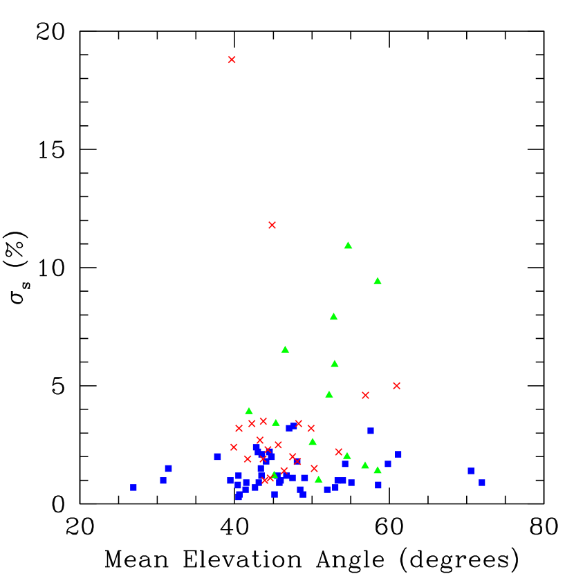
Figure 6: RMS scatter versus mean elevation angle. The fractional measured scatter of all our objects for the months of May and September is plotted against the mean elevation angle of the object for each month. Calibrator objects are shown as (blue) squares. Extended target galaxies are shown as (green) triangles, and point-like target galaxies are shown as (red) crosses. Objects observed at mostly low elevation angles do not exhibit higher levels of scatter, suggesting that self-calibration has been able to adequately compensate for variations in the atmosphere. (See the on-line paper for a color version of this figure.)

One possible source of apparent variability could be rapid phase fluctuations caused by the atmosphere which decrease the coherence by differing amounts from observation to observation as the weather changes. Since the calibrators are strong enough to be self-calibrated with very short solution intervals, this effect should only impact the target galaxies, and should affect low elevation sources the most, since the path lengths through the atmosphere are the greatest. Figure 6 shows the observed RMS level as a function of mean elevation angle for each month of observing for our sources. There is no significant increase in scatter for target galaxies, whether extended or point-like (“P” and “D” galaxies), at low elevation angles. NGC 777 (catalog NGC) has the two highest scatter values, but no other point-like targets have significantly high scatter at low elevation angles.

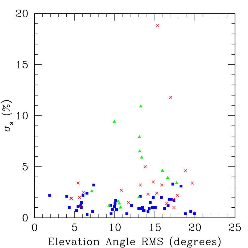
Figure 7: RMS scatter versus RMS elevation angle. The fractional measured scatter of all our objects for the months of May and September is plotted against the RMS variation in elevation angle of the object for each month. Calibrator objects are shown as (blue) squares. Extended target galaxies are shown as (green) triangles, and point-like target galaxies are shown as (red) crosses. There is no significant trend for objects observed at more varied elevation angles (and therefore more substantially different $(u,v)$ coverage) to have larger amounts of scatter in their measured flux densities. (See the on-line paper for a color version of this figure.)

Similarly, large changes in elevation angle from one observation to the next could be related to an increase in scatter caused by phase decoherence differences at different elevations, subtle gain problems depending on elevation, or even changes in the $(u,v)$ coverage of an object. Figure 7 plots the RMS scatter as a function of the RMS scatter in the elevation angle at which each galaxy is observed. Again, there is no significant trend visible in the data.

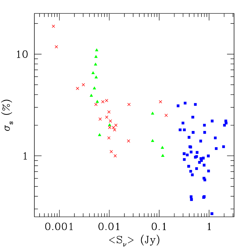
Figure 8: RMS scatter versus mean flux density. The fractional measured scatter of all our objects for the months of May and September is plotted against the mean flux density ($<S_{\nu}>$) for each month. Calibrator objects are shown as (blue) squares. Extended target galaxies are shown as (green) triangles, and point-like target galaxies are shown as (red) crosses. The objects with large variations in flux density all have mean flux densities less than about 8 mJy. However, only the two weakest point-like target galaxies show scatter levels above 4%, and it is unclear if this is a consequence of being unable to properly self-calibrate the weak targets NGC 777 and NGC 4565, or whether NGC 777 and NGC 4565 are just far more variable that the other galaxies in this survey. (See the on-line paper for a color version of this figure.)

Finally, it is expected that the scatter in the measured flux densities should be highest for the weakest sources. This could include a systematic coherence loss for those galaxies weaker than about 10 mJy where the signal to noise was potentially too low to use a solution interval short enough to track the phase variations of the atmosphere. Figure 8 plots the source flux-density scatter as a function of the mean flux density. The upper level of the scatter is uniformly about 4% for sources stronger than about 8 mJy. The four extended galaxies with $(u,v)$ related changes in flux density are all less than 8 mJy, creating the apparent spike for these objects. For point-like galaxies, only NGC 777 (catalog NGC) and NGC 4565 (catalog NGC) have RMS scatter levels above 4%. Unfortunately, they are also the two weakest sources, so we cannot clearly determine from this plot whether the high scatter is due to poor self-calibration or whether these objects are just more variable.

We adopt a $P_{\chi^{2}}$ upper limit cutoff of 0.01 to select sources which are variable at our sensitivity level. This cutoff corresponds to a 99% or greater confidence level in the variability. Disregarding J0410$+$7656 (catalog COINS), which is resolved and has known problems with varying $(u,v)$ coverage, none of the CSO sources has a $P_{\chi^{2}}$ value less than 0.01. Combining the May and September data, $10/28$ ($36\pm 9$%) of the non-CSO phase calibrators have $P_{\chi^{2}}<0.01$. Table 6 shows the variability fraction for various combinations of galaxy classifications. Although small number statistics prevent any definite conclusions being drawn about the fraction of extended and jet objects or core dominated objects, it seems that slightly more than half of our target galaxies show significant variability. Combining all of the reliable galaxies, $50\pm 11$% are variable. This fraction remains almost the same when the tentative galaxies are included, rising slightly to $57\pm 9$%.

The large fraction of target galaxies with $P_{\chi^{2}}\leq 0.01$ is not simply caused by an underestimation of the true measurement errors in the weak target galaxies. Our estimation of the true measurement errors appears to be valid, since several target galaxies actually have $\sigma_{\mathrm{e}}<\sigma_{\mathrm{s}}$, including three cases where the mean flux density was less than 10 mJy, and one case where some of observed scatter was caused by $(u,v)$ changes. Furthermore, the galaxies which do show variability often show coherent variations over several-day time-periods (for example, NGC 3031 (catalog NGC) NGC 3147 (catalog NGC) in September), something which would not be expected if the measurement error was simply underestimated.

Our results are in reasonably good agreement with other surveys of much stronger flat-spectrum ($\alpha>-0.5$) sources. Heeschen et al. (1987) found that $63\pm 8$% of their flat spectrum sources were variable at a $99.9$% confidence level ($P_{\chi^{2}}<0.001$) in their 1985 August and December observing sessions. As they point out, the amplitude of variability in their sample is very low—the maximum modulation index (often written as $m$ or $\mu$, with $m=\sigma/<S_{\nu}>$) they observed was only 3.4% in their flat-spectrum sample of 15 objects. We find that only 35% of our galaxies are variable at that confidence level, but their measurement error of about $0.27$% is about five times lower than ours. Quirrenbach et al. (1992) found similar results for objects in their sample, noting that sources with “compact” or “very compact” VLBI structures show substantially larger amplitude variations than sources extended on VLBI scales. In their survey of 118 compact, flat-spectrum sources, Kedziora-Chudczer et al. (2001) found that 19% of their sample showed variability above a 3-$\sigma$ level (roughly corresponding to $P_{\chi^{2}}<0.0005$). The vast majority of their sources have modulation indices at 8.6 GHz less than 2%. We find a slightly higher fraction of galaxies at this confidence level, even though our measurement errors are about a factor of two larger. Our “reliable” galaxies are compact on milliarcsecond scales, whereas the compact source sample of Kedziora-Chudczer et al. (2001) was taken from Duncan et al. (1993), which had a resolution of only $\sim 100$ mas, significantly larger than the VLBI scales used by Quirrenbach et al. (1992) to classify sources as “compact” or “extended”. Thus, our galaxies may show more variability because they are angularly smaller, as would be expected either for scintillation or intrinsic variability.

Since the flat spectrum objects appear to have a large percentage of objects varying at small modulation indices, this probably explains most of the differences in the fraction of variable sources detected by the different groups. Given these constraints, our results fit comfortably among these previous results, suggesting that it is quite likely that the variability we have observed is actually real. Other surveys looked at sources with flux densities $\gtrsim 1$ Jy, while our target galaxies are about two orders of magnitude fainter, so the results are not definitely conclusive as our weak target galaxies may have different properties.

In a slightly different comparison, Lovell et al. (2003) used the VLA to search for intraday variability in 710 compact flat-spectrum sources. Their first epoch of observations found that 12% of their sources show RMS variations above 4%. For our reliable target galaxies, 15% of the target-months show scatter levels above 4%, and 10% of the target-months show debiased scatter levels above 4%. This is in excellent agreement with the Lovell et al. (2003) results for substantially brighter sources. Again, this result highly suggests that the variability in our target galaxies is real, but cannot be conclusive.

5.3 Structure Functions

As an alternative to examining our data as a set of flux density changes as a function of time, we can transform our data into amplitude changes as a function of time separations (or lags) by using the so-called “structure functions”, a commonly used method to investigate the time behavior of variable radio sources. Since our data were not sampled at regular time intervals, we create a pseudo structure function as follows. We start with the first order structure function defined in the Appendix of Simonetti et al. (1985), which we modify to become

$$D^{(1)}(\tau)=\frac{1}{W^{(1)}(\tau)}\sum_{i=1}^{N}\sum_{j=i+1}^{N}w(i,j,\tau)\left[f(i)-f(j)\right]^{2},$$ (1)

where $f(i)$ is the fractional amplitude of the $i^{\mathrm{th}}$ observation, given by $f(i)=S_{\nu}(i)/<S_{\nu}>$, and

$$W^{(1)}(\tau)=\sum_{i=1}^{N}\sum_{j=i+1}^{N}w(i,j,\tau).$$ (2)

Since our observations were separated in a roughly logarithmic spacing scheme, we calculate our structure functions at logarithmic intervals, and use a weighting function given by

$$w(i,j,\tau)=\left\{\begin{array}[]{ll}1&\mbox{if\ }\log(\tau)-\zeta\leq\log\left[\mbox{JD}(j)-\mbox{JD}(i)\right]<\log(\tau)+\zeta\\ 0&\mbox{otherwise}\end{array}\right..$$ (3)

Here JD$(i)$ is the Julian Date of observation $i$, and $\tau$ is the time lag in days. The parameter $\zeta$ is an arbitrary number which must be at least half of the logarithmic spacing in $\tau$ in order to ensure that all data pairings are incorporated into the structure function. We set $\zeta$ equal to the spacing in $\log(\tau)$, $\log(\tau_{n})=n\zeta+\mbox{constant}$, $\zeta=0.125$ dex, in order to incorporate more data-points into each interval and partially smooth the structure function.

The uncertainty in the structure function is given by

$$\delta D^{(1)}(\tau)=\frac{2}{W^{(1)}(\tau)}\left\{\sum_{i=1}^{N}\sum_{j=i+1}^{N}w^{2}(i,j,\tau)\left[f(i)-f(j)\right]^{2}\left[\delta f^{2}(i)+\delta f^{2}(j)\right]\right\}^{1/2},$$ (4)

where $\delta f(i)$ is the measurement uncertainty in observation $i$. For observations with nonzero measurement errors, the computed structure function will be biased above the true level, as $\left[f(i)-f(j)\right]^{2}$ does not average to zero. This bias is given by

$$D_{\mathrm{bias}}^{(1)}(\tau)=\frac{1}{W^{(1)}(\tau)}\sum_{i=1}^{N}\sum_{j=i+1}^{N}w(i,j,\tau)\left[\delta f^{2}(i)+\delta f^{2}(j)\right].$$ (5)

If the measurement errors are the same for all data-points, then these equations reduce to the ones shown in Simonetti et al. (1985).

Figure 9 shows the structure functions for our 18 target galaxies. The structure function values are shown as individual points with error-bars, but have not been corrected for measurement bias. The estimated bias levels are shown by the lines going across each plot. One can immediately see that the structure functions are quite complicated. This is partially a result of the relatively low signal to noise of our faint target galaxies compared with other intraday variability observations.

Galaxies such as NGC 2273 (catalog NGC) and NGC 3227 (catalog NGC) which have variability caused by $(u,v)$ effects typically have structure function values an order of magnitude above the bias level, while galaxies such as NGC 3079 (catalog NGC) and NGC 4168 (catalog NGC) which have been classified as constant have structure function values consistent within the error-bars with the bias levels. The majority of target galaxies have structure function values at or below the estimated bias level for short time-lags, up to a day or a few days. This suggests that our flux-density uncertainty levels are not underestimated, and in fact they may be slightly overestimated. We are therefore confident that the $P_{\chi^{2}}$ probabilities and de-biased scatter levels are trustworthy.

6 Physical Interpretations of the Variability

Having established that variability is present in many of our target galaxies, we now investigate implications this variability has for the physical properties of the radio emission regions. We will treat possible intrinsic and extrinsic variations in turn.

6.1 Intrinsic Implications: Brightness Temperature

One potentially important piece of information about the radio emission is the brightness temperature of the source. Some LLAGN models such as the simple ADAF model suggest that the observed radio emission is produced by synchrotron emission from thermal electrons. In this case, the bulk of the observed emission comes from the region where the optical depth reaches about unity, and the observed brightness temperature should not be too different from the thermal temperature of the electrons, which is expected to be a few times $10^{9}$ K (see, e.g. Mahadevan, 1997). However, if a significant population of nonthermal electrons is present, as expected for more complex ADAF and jet models, the brightness temperature could easily exceed this value. Results from VLBA imaging of our target sample have found lower limits to the brightness temperature of $10^{8}$–$10^{9}$ K (see Table 3 of this paper, Table 4 of Anderson et al., 2004, Table 1 of Falcke et al., 2000). These VLBI measurement limits are unfortunately unable to discriminate between current models.

Assuming that the variability we observed with the VLA is real and intrinsic to the source, then the variability can improve our understanding of the physical conditions in the source region smaller than the VLBA observations can resolve. The brightness temperature is given by

$$T_{\mathrm{b}}=\frac{S_{\nu}\lambda^{2}}{2k\Omega}=\frac{S_{\nu}c^{2}}{2k\Omega\nu^{2}},$$ (6)

where $\Omega$ is the solid angle of the emission region. Suppose that a source changes in flux density by an amount $\left|\Delta S_{\nu}\right|$ in a time $\Delta t$. The speed of light provides an upper limit to the size of the variable radio source, with a maximum solid angle for a distant, unbeamed, variable region of

$$\Omega\leq\frac{\pi\left(c\Delta t\right)^{2}}{D^{2}},$$ (7)

where $D$ is the distance to the source. (This ignores relativistic beaming effects — probably a good assumption for most LLAGNs since most Seyfert galaxy jets generally appear to be relatively slow; see Ulvestad, 2003.) The lower limit to the brightness temperature of the variable component of emission is then

$$T_{\mathrm{b}}\geq\frac{D^{2}}{2\pi k\nu^{2}}\left(\frac{\left|\Delta S_{\nu}\right|}{{\Delta t}^{2}}\right),$$ (8)

where the information in parentheses must be determined from the observed time series. As an example, during the first day of observations in 2003 May, NGC 777 (catalog NGC) went from 0.52 mJy to 0.87 mJy in 0.079 days (see Figure 2), corresponding to $T_{\mathrm{b}}\geq 5\times 10^{13}$ K, far in excess of the inverse-Compton limit (see, e.g. Kellermann & Pauliny-Toth, 1968). Many other target galaxies also have similar implied instances of brightness temperatures above $10^{12}$ K.

However, because our target galaxies are relatively weak, the relative uncertainty in $\left|\Delta S_{\nu}\right|$ is very significant. Formal error analysis indicates that for the NGC 777 (catalog NGC) data mentioned above, the $\left|\Delta S_{\nu}\right|$ value is a 2.6-$\sigma$ difference. If we assume that NGC 777 (catalog NGC) was actually constant during our observations, random error in the flux density difference would produce a brightness temperature measurement of at least $10^{12}$ K 48% of the time. Two additional flux density differences in NGC 777 (catalog NGC) also suggest brightness temperatures above $10^{12}$ K, but similar error analysis suggests that $10^{12}$ K temperatures would be found 44% and 41% of the time for a constant source. At first glance, it seems unlikely that all three measurements would be above $10^{12}$ K — the combined probability that none of the three are indeed above $10^{12}$ K is only 17%. Although this seemingly suggests that it is likely that NGC 777 (catalog NGC) has a variable emission region with $T_{\mathrm{b}}\geq 10^{12}$ K, such an analysis is flawed, because it does not take into account the statistics of all possible data pairings.

There are 191 possible combinations of measurement points which can be used to calculate brightness temperatures for NGC 777 (catalog NGC) (although there are actually 378 pairings of NGC 777 (catalog NGC) data-points, differences between May and September data-points are unlikely to yield interesting brightness temperature limits). We therefore expect measurement noise to cause two 2.6-$\sigma$ or larger differences to appear in the NGC 777 (catalog NGC) dataset if NGC 777 (catalog NGC) was actually constant in flux density. Thus, the modest signal to noise levels of our data prevent us from simply relying on calculating the brightness temperature limits for only those difference-pairs above some threshold (such as 5-$\sigma$) to give an accurate estimate of the brightness temperature of variations in the target galaxies.

In order to assess the effect of the multitude of statistical opportunities to artificially generate high brightness-temperature point differences, we created two slightly different Monte Carlo simulations of our LLAGN datasets. In the first simulation, a set of random measurement errors is created from a normally-distributed random number generator according to the actual measurement uncertainties in the real dataset. Then, using an assumed underlying brightness temperature and the observation dates from the original dataset, a simulated flux density difference including the random measurement errors is calculated for each pair of measurements. This effectively assumes that every pair of measurement points has the equivalent of a flare starting at one point, and growing in intensity to the second point. (Increases or decreases in flux density are mathematically equivalent in the $\left|\Delta S_{\nu}\right|$ model, so only rises are implemented to maintain consistency.) Next, the simulated difference pairs are numerically analyzed, and the number of difference pairs which have a simulated measurement difference above a minimum brightness temperature threshold and a measurement flux density difference above a specified sigma level are counted. The results are recorded, and the same process is repeated for a total of $10\,000$ trials using different random measurement errors.

This simulation process is then repeated again for a slightly higher assumed brightness temperature, and so on, until a wide range of assumed brightness temperatures has been covered. Once these Monte Carlo simulations are finished, the results are compared with number counts from the real dataset using the same selection criteria as for the simulated datasets. For low assumed brightness temperatures, the simulated datasets have low simulated brightness temperature measurements and most of the flux density differences have small sigma levels, so that far fewer pairs are counted above the threshold compared to the real dataset. For high assumed brightness temperatures, the situation is reversed as the random measurement errors are small compared to flux changes required by the high assumed brightness temperature and many pairs are counted above the threshold. We find the assumed brightness temperature at which the mean count number (above threshold) from the Monte Carlo simulations matches the count number from the real dataset, giving us the best estimate of the brightness temperature implied by variations in the real dataset. We also determine the brightness temperature for which 10% of the Monte Carlo simulations have a count number at least as high as the real dataset, giving us a 90% confidence estimate that the actual brightness temperature of the fluctuations in the real dataset is at least this high.

Because this algorithm assumes that every pair of data-points contains a “flare” at the assumed brightness temperature, it will tend to predict more data pairs which exceed our counting threshold than would be seen in a real target having some quiescent periods. Looking at the time series of the target galaxies for which we have good confidence that the variability is real, the measured flux density does not continuously rise or fall, but instead tends to both rise and fall over a characteristic timescale from a few hours to a few days. This suggests that intrinsic processes which lead to variability in our target galaxies may be causing new sources of emission to appear and fade away over the course of our observations. Furthermore, it is possible that “flares” do not start at one of our data-points, but begin somewhere between our observation times. Thus, not all pairs of data-points should show variations of the assumed brightness temperature, as there should be periods when the flux density is neither rising nor falling, but is roughly constant, with other periods of somewhat rising and somewhat falling values.

To make a first order correction for this effect, we have performed a second Monte Carlo simulation. We assume that each data pair contains a random amount of emission up to the assumed brightness temperature. The generating function for the physical brightness temperature distribution for data pairs is probably a complicated function of the prior history of the variations and the time difference between the data points. But for our first order correction, we simply use a uniform random number generator to create a variable emission temperature between zero and the assumed brightness temperature. Otherwise, this second Monte Carlo simulation follows the same prescription as the first simulation.

Table 7 shows the results of these simulations. The first simulation results are shown in Columns (6) and (7), giving the 50% (best) and 90% (minimum) confidence estimates of $T_{\mathrm{b}}$, respectively. Columns (8) and (9) give the results for the random brightness temperature simulation. Attempting to deal with all biases, Columns (8) and (9) are our best estimates of the variability brightness temperatures. They are always higher than those in Columns (6) and (7) because a higher brightness temperature is needed to “compensate” for the hypothesized quiescent periods. Blank values indicate that the simulation result for the brightness temperature was less than the $10^{5}$ K minimum simulation temperature. These results are from simulations with a $2.5$-$\sigma$ flux-density difference threshold and a temperature threshold of the assumed brightness temperature. Simulations with other thresholds ($1.5$-$\sigma$ to $3.5$-$\sigma$ and various temperature schemes) show essentially the same results, having brightness temperatures generally within a factor of 2 (0.3 dex) of the values in Table 7. (Calculations using different error distributions give essentially the same results. See Appendix B.) For comparison, Columns (4) and (5) show the results from a direct analysis of the observed flux density variations in the target datasets, showing the first highest and fourth highest apparent brightness temperatures from all dataset pairings.

For the target galaxies that we are confident show real variability (the “var” galaxies), the brightness temperatures from the Monte Carlo simulations are typically somewhat larger than the lower limits determined from VLBI observations, but they are still potentially consistent with most accretion and emission models for LLAGNs. The best estimates of the brightness temperatures are between about $10^{9}$ and $10^{11}$ K, with the 90% confidence limits about half a dex lower. Although $10^{10}$ K is higher than the general expectation from simple thermal electron ADAF models, physical electron temperatures this high are possible when the accretion rate approaches about $10^{-2}$ Eddington (see, e.g., Figure 2 of Mahadevan, 1997).

The brightness temperatures calculated here are also interesting in terms of the inverse-Compton limit, which constrains the brightness temperature of an incoherent-synchrotron emission source to a maximum value of about $10^{12}$ K (Kellermann & Pauliny-Toth, 1968). If the magnetic field energy density is approximately in equipartition with the particle energy density, the brightness temperature limit is about an order of magnitude less, as suggested by Readhead (1994), Begelman et al. (1994), and Sincell & Krolik (1994) (these papers suggest limits of about $6\times 10^{10}$ K, $10^{11}$ K, and $9\times 10^{10}$ K, respectively, for our LLAGNs). Only NGC 5866 (catalog NGC) (whose variability we classify as tentative) approaches the $\sim 10^{12}$ K inverse-Compton limit. The remaining galaxies are all below the equipartition limit of about $10^{11}$ K, and for the 90% confidence limits to the brightness temperature, none of the variable galaxies exceed the equipartition limit.

We would like to reiterate that these brightness temperatures are probably lower limits to the actual brightness temperatures of the emission regions responsible for the variability. Equation 7 assumes that the variable region of emission expands spherically at a velocity of $c$. Since we have no way to measure the actual size of the emission region if the variability is intrinsic to the target galaxy, the emission region could well be smaller than this maximum limit, the actual brightness temperatures thereby being substantially higher than those listed in Table 7. Furthermore, if there are multiple, independent regions of variable emission, the sum of all of the emission from the target galaxy core would tend to have smaller fluctuations as the individual variations would tend to cancel one another out. Finally, we would like to emphasize that the brightness temperatures determined in this section are for the regions of variable emission, and do not give any information about regions of constant emission. This constant emission could have a brightness temperature significantly different than the variable emission, depending on the physical processes leading to the constant and variable emission.

6.2 Extrinsic Variability: Interstellar Scintillation

An alternative variability explanation is refractive interstellar scintillation of the radio emission, caused by density perturbations in the Galactic interstellar medium, which distort the wavefront of radio waves passing through the medium. As the interstellar medium appears to move across the line of sight toward a source (because of the relative motion between the Sun and the ISM and the orbital motion of the Earth), the observer sees alternating regions of increased or decreased apparent brightness of the source. Reviews of this process can be found in Rickett (1990), Narayan (1992), and references therein. The variability in some extragalactic sources has now conclusively been attributed to refractive scintillation (see, e.g. Rickett et al., 2001; Dennett-Thorpe & de Bruyn, 2001, 2002; Jauncey et al., 2003) If significant amounts of the core flux come from a region smaller than several tens of microarcseconds across on the sky, our target galaxies have a good possibility of showing refractive scintillation in our measurements. Using properties of the scatter behavior in the observational data and making some assumptions about the Galactic interstellar medium in the direction of target galaxies gives estimates of the solid angles subtended by the sources on the sky for extrinsic variability.

In our relatively simple analysis, we follow the discussions in Walker (1998, see also the errata notice in ) and Rickett (2002). For weak scattering caused by a single, thin region of the ISM, the refractive medium will cause waves propagating toward the observer to constructively and destructively interfere on a characteristic angular size scale. This scale is related to the size of the first Fresnel zone, which is given by

$$\theta_{\mathrm{F}}=1/\sqrt{Lk},$$ (9)

where $k$ is the wavenumber of the radio waves and $L$ is the distance to the ISM screen. Converting to frequency in units of gigahertz and distance in kiloparsecs, the angular size in microarcseconds is $\theta_{\mathrm{F}}\approx 8.11/\sqrt{L\nu}$. As the ISM screen moves across the line of sight toward the source with a transverse velocity relative to the observer of $v$, the screen will appear to move a distance equal to the characteristic angular size scale in a time

$$t_{\mathrm{F}}=v^{-1}\sqrt{L/k}.$$ (10)

With the velocity in kilometers per second, frequency in gigahertz, and distance in kiloparsecs, the timescale in days is given by $t_{\mathrm{F}}\approx 14.0\,v^{-1}\sqrt{L/\nu}$.

Following Rickett et al. (1995), we have adopted a transverse velocity of $50$ km s^-1 to account for the relative motions of the Earth about the Sun, the motion of the Sun with respect to the local standard of rest, and the velocities of plasma clouds within the ISM. Using the NE2001 software from Cordes & Lazio (2002), which contains a model of electron densities and fluctuations in the ISM, we have calculated effective distances to phase screens for the lines of sight to our extragalactic sources, and hence values for $\theta_{\mathrm{F}}$ and $t_{\mathrm{F}}$. We also used NE2001 to calculate the transition frequency ($\nu_{0}$) between strong and weak interstellar scattering (see, e.g., Rickett, 2002). These quantities are shown in Table 8. Our values are in basic agreement with the plots in Walker (2001) which are based on the older Galactic electron density model of Taylor & Cordes (1993).

It is important to recognize that we do not have exact knowledge about the ISM screens which might be causing scintillation of our target galaxies. Detailed studies of individual objects undergoing strong scintillation have shown that the transverse velocities and distances of the screens are often substantially different from the “expected” values. However, we hope that the results we obtain using our NE2001-based predictions will be reasonably correct on average. The angular size information is only proportional to the square root of the screen distance, so distance errors of a factor of ten will result in size errors of a factor of three. The screen velocity could easily have errors of a factor of a few. Also, since the transition frequency is close to the observation frequency, it is not clear whether the scintillation is actually in the weak or strong regime, so another error factor of about two may be possible. Added in quadrature, the size estimate error for any specific object should be less than about a factor of five, assuming that the variability is entirely due to interstellar scattering.

We expect that the intrinsic sizes of the emission regions of our target galaxies will be substantially larger than the Fresnel angle ($\theta_{\mathrm{F}}$). In this case, the integrated brightness of the target emission will be the sum over many different regions of the plasma screen. The scintillation effects of each area of the screen are relatively independent, so the brightness variations caused by each Fresnel angular region will tend to cancel one another. This causes the amplitude of the variation to decrease and the timescale of the variation to increase roughly as the square root of the number of independent Fresnel zones for a uniformly illuminated source. Since the number of Fresnel zones will go as the square of the source angular size, the variations will depend on the source size to roughly the first power. Taking the equations for weak scattering from Walker (1998), the angular size of the source based on a measurement of the variability timescale $\tau_{\mathrm{max}}$ is

$$\theta_{\tau}=\frac{\tau_{\mathrm{max}}}{t_{\mathrm{F}}}\theta_{\mathrm{F}}.$$ (11)

Similarly, an alternate estimate of the source angular size is given by the modulation index, which is just our de-biased scatter from § 5.1. Scintillation theory predicts

$$\theta_{m}=\left(\frac{m_{\mathrm{p}}}{m}\right)^{6/7}\theta_{\mathrm{F}},$$ (12)

where $m_{\mathrm{p}}$ is the expected modulation index for a point source; $m_{\mathrm{p}}=\left(\nu_{0}/\nu\right)^{17/12}\sim 100\%$ since our observing frequency is close to the predicted transition frequency.

The variability timescales were estimated by eye from the structure function plots in Figure 9. For interstellar scintillation, the structure function at small time lags is expected to rise as a function of the time lag to some power (a straight line in a log-log plot), rising to a maximum at the characteristic timescale of variability for the object, followed by a plateau region at a value $2m^{2}$ (see, e.g., Beckert et al., 2002). Our target galaxies generally have noisy structure functions which do not allow for a simple deduction of the timescale of the initial maximum. In Table 8 we report the lag ($\tau_{\mathrm{max}}$) for the initial peak in the structure function with values clearly above the observational bias levels. Because the structure function values for timescales longer than 10 days are generally poorly sampled, peaks occurring at timescales larger than 10 days have been indicated by a lower limit symbol.

Using the scintillation model predictions and our $\tau_{\mathrm{max}}$ and $m$ measurements, we calculated angular sizes of our target galaxies. Table 8 shows the results of these calculations for the targets which show significant variability ($P_{\chi^{2}}<0.01$). Our calculations assume that all of the emission comes from a compact core, as suggested by VLA and VLBA measurements which have similar flux densities. If part of the emission is from an extended emission region (say more than about 1 mas in size), the interstellar scattering would only affect the remaining compact core, which would decrease the measured modulation index, and therefore increase the angular size of the compact core calculated from the modulation index. The angular size calculated from the variability timescale would remain unchanged.

If weak interstellar scattering is responsible for the variability in our target galaxies, then $\theta_{\tau}$ and $\theta_{m}$ should have approximately the same value. The two methods generally agree with one another within a factor of 10, although there is one case where $\theta_{m}\sim 40\,\theta_{\tau}$. Equations 9 and 10 have inverse dependencies on the distance $L$ to the ISM screen, so in principle the distance to the screen could be found if one believes both the $\tau_{\mathrm{max}}$ and $m$ measurements. Of the 16 variability instances in Table 8, 9 have $\theta_{\tau}<\theta_{m}$, so there is no significant tendency for either $\theta_{\tau}$ or $\theta_{m}$ to be too large or small. This suggests that the distance estimates from the NE2001 software are probably not significantly biased high or low.

Assuming that the angular size calculated from the modulation index is approximately correct, we have also calculated the equivalent radius of the emission region, assuming that the source is circular on the sky. The linear radius is given in units of Schwarzschild radii in Table 8, as this quantity is more likely to be of interest for comparison with LLAGN models. The radii have a mean of 540 $R_{\mathrm{S}}$, and range from 38 to 1200 $R_{\mathrm{S}}$. Given the range of black hole masses, target galaxy distances, and calculated angular sizes, the range in radius seems relatively small, but we have not performed a careful analysis of observational biases which might limit the range in radius we could measure. A typical radius of 500 $R_{\mathrm{S}}$ is in reasonable agreement with predictions for ADAF sizes at 8 GHz. However, as described above, the variability timescale and modulation index resulting from interstellar scintillation are actually most dependent on the area (solid angle) of the source on the sky, rather than a one-dimensional angle. The exact shape of the emission on the sky is not constrained by our measurements, so the target galaxies could also have an elongated structure, as would be expected from jets. Therefore, the targets could also have a major to minor axis ratio of $\sim 5$ and still be within the angular size limits from our VLBA observations. This means that jet-like structures are also still allowed from the size restrictions from our interstellar scintillation calculations.

Since the brightness temperature of the emission depends on the solid angle of the source, the brightness temperature derived from the interstellar scattering size estimate is valid whether the source is circular or elongated. Table 8 shows the brightness temperatures derived in this way. Remarkably, the brightness temperatures are also reasonably constant, with a mean of $10^{10.6}$ K and a standard deviation of only a factor of 3. There are no galaxies which appear to have brightness temperatures above the inverse Compton limit of $\sim 10^{12}$ K. (Brightness temperatures as high as $10^{14}$ K could have been detected in our sample galaxies.) Although these brightness temperatures are moderately high for the standard ADAF models, they can probably be accommodated with the inclusion of a small non-thermal electron population. Alternatively, these brightness temperatures are quite reasonable for jet models.

The differences of up to a factor of 40 between $\theta_{\tau}$ and $\theta_{m}$ seem rather larger than we would expect for good agreement between the two methods of calculating angular size. The structure function plots for our targets are very noisy, which is partially due to the small flux density changes we are measuring. The structure on short timescales may also be affected by other things besides interstellar scattering, such as problems in the instrumentation or intrinsic flicker in the target galaxies. Whatever the cause, the $\tau_{\mathrm{max}}$ estimates for the structure function plots in Figure 9 are probably not very reliable. We have somewhat better faith that the modulation index calculations for the variability are closer to being correct, as the modulation index contains information from all of the data-points, while the individual structure function points depend on only a few measurements each. The modulation-index-based angular sizes in Table 8, which assume that all of the variability is caused by interstellar scattering, have a mean angular size of 76 $\mu$as. However, the structure functions for our targets do not show the expected power law rise at small time lags. This may be caused by at least some of the variability being intrinsic to the target emission regions. In that case, the fractional variability due to scintillation would be smaller than $\sigma_{\mathrm{d}}$, which would increase the sizes of the emission regions. Therefore, sizes in Table 8 should be treated as probable lower limits, and brightness temperatures as upper limits.

6.3 Extrinsic or Intrinsic Variability?

Intrinsic variability is a viable explanation for the variability we observed in the nuclear emission regions of our galaxies. The inferred brightness temperatures are in the range $10^{9}$–$10^{11}$ K — less than the inverse Compton limit. The roughly few days timescale of the variability as measured from the structure functions implies a variable emission region size smaller than about 50 $\mu$as for the typical distance of our sample galaxies, which is well within the size limits from our VLBA observations. The total extent of the radio emitting region can, however, be significantly larger than this size.

Scintillation-induced extrinsic variability is also consistent with our observations. Most of our “reliable” galaxy datasets show variability in at least one epoch, and we use this information to estimate the sizes for all of our galaxies. (Because the scintillation seen in some IDVs is known to be transient, we expect some galaxies which could scintillate to actually remain constant, see Kedziora-Chudczer et al., 1997, 2001.) Assuming all of the variability is caused by scintillation, the mean angular size is 76 $\mu$as, and the brightness temperature is $10^{10.6}$ K. Once again, the brightness temperatures are below the inverse Compton limit.

Thus, whether the variability is extrinsic or intrinsic, the implications for the physical conditions of the emission regions are approximately the same. Furthermore, large Doppler boosting factors are unnecessary to explain the brightness temperatures, which are comfortably within even the equipartition inverse-Compton limit of Readhead (1994) and others. This is in stark contrast to intraday variability observations of bright, distant AGNs which occasionally imply apparent brightness temperatures of $10^{19}$ K or higher (see, e.g., Wagner & Witzel, 1995). In such cases, interstellar scintillation is normally preferred over intrinsic variations to explain the origin of the variability, as it predicts dramatically larger angular sizes and reduces the necessary Doppler factors.

As discussed in § 6.2, we believe that at least some intrinsic variability is present in our galaxies based on their structure function behavior. We therefore combine our information to come up with our best estimates of the physical parameters of the LLAGN emission at $8.5$ GHz for our VLBA unresolved nuclei. The VLBA imaging typically gives upper limits of $0.5$–$0.7$ mas for the major axis of the emission region. The scintillation results give a mean lower limit of $0.076$ mas. Correcting for a reasonable amount of contamination by intrinsic variability, we estimate that the mean actual size of the emission regions is $0.2$ mas, plus or minus a factor of two for individual galaxies. In terms of mean linear size, this is about 1400 $R_{\mathrm{S}}$ plus or minus a factor of two.

This corresponds to an estimated solid angle of about $0.04$ mas², which is potentially more meaningful, since the scintillation results are shape-insensitive. The emission can therefore be circular on the sky or in a narrow strip. For jet models, this allows the emission to extend out to a distance of $0.5$ mas (or $1.0$ mas in the case of NGC 5866 (catalog NGC)) so long as the emission is only $0.08$ mas ($0.04$ mas) wide. This suggests that the mean brightness temperature is about $10^{10.1}$ K, with individual galaxies being perhaps plus or minus $0.6$ dex different. This well matches the brightness temperature findings from intrinsic variability and is consistent with the lower limits from our VLBA imaging.

A brightness temperature of $10^{10.1}$ K is close to an order of magnitude higher than expected from the traditional ADAF model with electrons in a thermal energy distribution. Thus, our results require an additional population of high-energy non-thermal electrons in order to produce the observed brightness temperatures. Whether this non-thermal electron population is present in the accretion disk, or in an outflow from the accretion disk, or in a jet remains an open question.

Our results compare favorably with other results for the sizes of compact LLAGN. VLBA measurements of the size of NGC 3031 (catalog NGC) are discussed in Appendix C. For Sgr A^∗, Bower et al. (2004) claim to have measured the size of the emission region at high frequencies using the VLBA. Their fit to the angular size of Sgr A^∗ predicts a major axis size of 160 $R_{\mathrm{S}}$ in radius at our observing frequency of 8.46 GHz. Sgr A^∗ has a radio luminosity about $10^{5}$ times weaker than the median target galaxy in our sample, the black hole mass for Sgr A^∗ is about 10 times smaller than the typical black hole mass in our sample, and the emitting region is $10^{3}$–$10^{4}$ times closer. Therefore, the brightness temperature of Sgr A^∗ at 8.46 GHz is still close to the brightness temperature of our objects. It is possible that the size of the radio emission region scales with black hole mass and radio luminosity over an extremely wide range of luminosities and mass accretion rates.

7 Medium-Term Variability

Active galactic nuclei are well known for having variable emission at all observed frequencies (see, for example, the review by Ulrich et al., 1997). In addition to the short intraday variability, AGNs typically also show relatively large amplitude variations over longer timescales, from months to years. As with other wavelength regimes, long-term radio variability in low-luminosity AGNs is less well studied, but is known to be present, as indicated by the studies of Nagar et al. (2002) who found that almost half of their LLAGN sample observed with the VLA at 8.5 GHz changed in flux density by at least 20% after a 15 month time interval.

Many of our own LLAGN target galaxies also changed significantly from the May to September variability runs. To measure this effect, we calculated the average flux density from the last three days of our 2003 May observations and the average flux density from the first three days of our 2003 September observations. These days had the most similar $(u,v)$ coverage between the two months, with most of the VLA antennas in their A configuration locations. Therefore, these three day averages should minimize $(u,v)$ differences, and provide reliable flux density estimates to compare all of our target galaxies. Averaging over several days for each month should also minimize variations caused by short-term variability, whether intrinsic or extrinsic in origin.

Fractional variation values were calculated from

$$F=\frac{2\left(<S_{\mathrm{Sep}}>-<S_{\mathrm{May}}>\right)}{<S_{\mathrm{Sep}}>+<S_{\mathrm{May}}>},$$ (13)

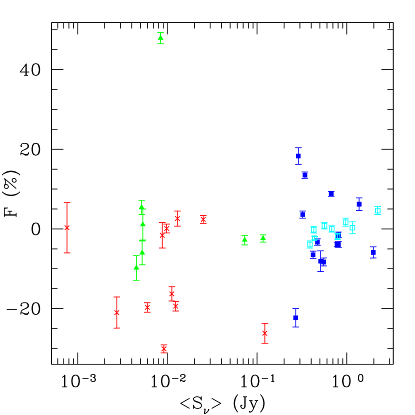
Figure 10: The long-term fractional variation is plotted as a function of mean flux density. Negative values indicate that the source was weaker in 2003 September than 2003 May. Calibrator objects are shown as squares, with CSO calibrators indicated by open (cyan) squares and non-CSO calibrators by solid (blue) squares. Extended target galaxies are shown as (green) triangles, and point-like target galaxies are shown as (red) crosses. (See the on-line paper for a color version of this figure.)

along with associated uncertainty estimates. These values are listed in Table 5, and plotted as a function of mean flux density in Figure 10. The CSO calibrators all have fractional variations less than 5%, and are centered about $F=0$, suggesting that the absolute flux density calibration of both months was performed properly. The other phase calibrators tend to be more varied. Roughly equal numbers of calibrators increased (positive $F$) and decreased (negative $F$) in flux density from May to September.

The fractional variations of the target galaxies are rather different. Seven of the eighteen target galaxies have flux density changes of more than 10% from May to September. Of these galaxies, only one (NGC 3226 (catalog NGC)) increased in brightness, while six decreased substantially over the time period. The random probability that at least six of seven galaxies would all increase or decrease is 13%, so the apparent excess of decreasing flux densities is not statistically significant. None of these seven galaxies have short-term variability related to $(u,v)$ effects, and the target galaxy changes do not appear related to changes in the flux densities of their phase calibrators. After carefully examining the data, and remembering that the numbers of calibrators with increasing and decreasing flux densities are about equal, we are confident in the measured fractional variations of these galaxies.

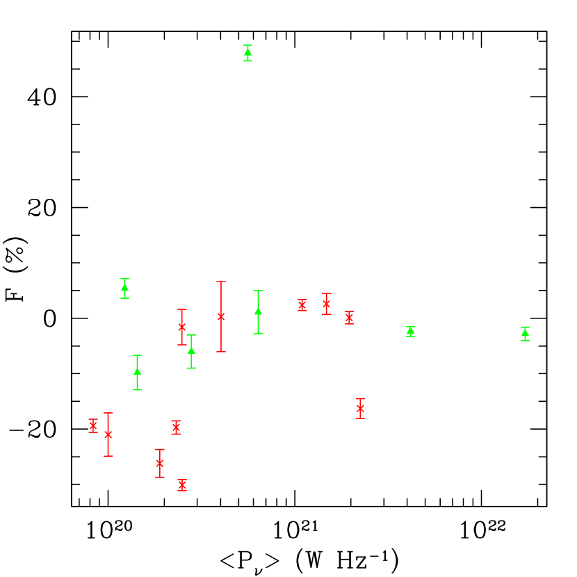
Figure 11: The long-term fractional variation is plotted as a function of mean radio luminosity. The radio luminosity ($P_{\nu}$) was calculated assuming isotropic radiation. Extended target galaxies are shown as (green) triangles, and point-like target galaxies are shown as (red) crosses. (See the on-line paper for a color version of this figure.)

The probability that a target galaxy would change dramatically between the two observation periods does not seem to be related to the observed flux density, as the large fractional variations occur over essentially the entire target flux-density range. However, Figure 11 shows that most of the large fractional variations occur in the galaxies with the weakest 8.5 GHz luminosities in our sample. We are unsure whether this result is a real effect or just coincidence, although it might be possible that the weakest galaxies are able to vary more easily over the $\sim 4$ month timespan between our observations.

Barvainis et al. (2004, hereafter B04) have completed a study of the long-term variability of AGNs to search for possible differences between radio-loud and radio-quiet AGNs. Radio loudness is defined here as the ratio $R$ between radio and optical flux densities (Kellermann et al., 1989), with $R<3$ defining a radio-quiet quasar (RQQ), $3<R<100$ defining a radio-intermediate quasar (RIQ), and $R>100$ defining a radio-loud quasar (RLQ). The AGNs used in B04 range from “classical” Seyfert galaxies to bright quasars. They find no significant differences between the radio core variability and spectral index properties as a function of the radio-loudness parameter $R$.

Our study extends the results in B04 by identifying the variability statistics for flat-spectrum LLAGNs, which are significantly lower in luminosity, extending the range of radio luminosities examined by about 1.5 orders of magnitude to weaker sources. Although the radio powers of our LLAGN cores are weak, the ratios of radio to optical flux densities classify our galaxies as radio-loud or radio-intermediate (see Ho, 2002). Our galaxies are some four orders of magnitude fainter than the weakest radio loud AGN of B04. The combined range of radio-loud radio luminosities is therefore about 8 orders of magnitude, from $10^{20}$–$10^{28}$ W Hz^-1.

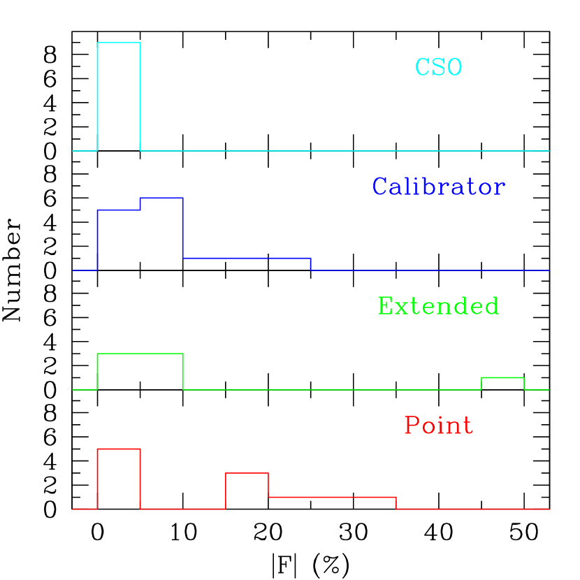
Figure 12: Histogram of the number of sources as a function of the absolute long-term fractional variation. CSO calibrators have been separated from non-CSO calibrators, and extended galaxies are separated from point-like galaxies.

The amplitude of medium-term variability seen in Figures 10 and 11 is quite similar to the variability found by Barvainis et al. (2004), accounting for the differences between our fractional variation $F$ and their de-biased RMS variability. Figure 12 presents a histogram of the number of sources as a function of the absolute fractional variability. Combining our extended and point-like results, our medium-term sample variability results are quite similar to the results of B04, given the small number statistics. Our variability results for our non-CSO calibrators are also similar to their results.

The quasars investigated in B04 tend to be located at cosmological distances (redshifts in the range $0<z<4$), while our most distant galaxy is only 66.5 Mpc away ($z=0.017$). Thus, our VLA observations measure emission on much smaller physical scales than the B04 observations. However, large-scale jet emission tends to have a steep spectral index, so the B04 study should be dominated by core emission at 8.5 GHz. Furthermore, Ulvestad et al. (2004) find that most of the radio-quiet quasars they have investigated with the VLBA are consistent with all of the arcsecond (VLA) scale flux density being located in the milliarcsecond (VLBA) scale core. Thus, our VLA observations are actually measuring emission from the same size scales as the B04 observations.

Although a more detailed long-term study of variability in LLAGNs is needed, our results indicate that both the medium- and short-term variability properties of LLAGNs are similar to those of far more luminous quasars. The radio spectral indices of the nuclear regions of Seyfert LLAGNs (Ulvestad & Ho, 2001a) are also similar to the quasar sample in B04, with approximately equal numbers of sources with spectral indices above and below $\alpha=0$ and concentrated in the range $-1<\alpha<+1$. These results suggests that the physical processes responsible for producing the observed radio emission from AGN cores may be the same for all AGNs, despite a luminosity range of some 8 orders of magnitude. However, the luminous quasars have combined optical and X-ray luminosities which are close to the Eddington limit (for radio-quiet as well as radio loud quasars, see Ulvestad et al., 2004), while our low-luminosity AGNs have bolometric luminosities orders of magnitude below the Eddington limit. It is not clear that the accretion processes which lead to the optical and X-ray emission are necessarily related to the processes which lead to the radio emission ubiquitously seen in AGNs.

8 Conclusions

We have conducted a VLA variability study of a sample of 18 predominantly flat-spectrum LLAGNs to investigate the sizes of the radio emission regions in these objects. Our analysis included new and published milliarcsecond-scale VLBA imaging of all 18 objects.

The majority of our sample galaxies have essentially all of their large (arcsecond) scale flux confined within a single, sub-milliarcsecond core. NGC 2273 (catalog NGC) and NGC 3227 (catalog NGC), which have steep radio spectral indices ($\alpha\leq-0.5$) on VLA scales, have extended structure on VLBA scales, as does NGC 3079 (catalog NGC). Three of our galaxies have measured sizes from our VLBA observations of $\sim 1.5$ mas in the major axis, and are effectively unresolved in the minor axis. The 11 remaining galaxies with VLBA detections all have sizes less than 1 mas and are probably smaller than $0.5$ mas.

We have detected short-term variability in our LLAGN sample on time scales from slightly less than a day to 10 days. The fraction of galaxies which are variable at or above the 4% level agrees very well with a larger sample of far more luminous AGNs performed by Lovell et al. (2003). The fraction of galaxies with smaller variability amplitudes also agrees quite well with other existing studies of more luminous AGNs.

The observed variability is consistent with intrinsic variability, but is also partially consistent with scintillation caused by the Galactic interstellar medium. Both intrinsic and extrinsic (scintillation) explanations for the variability yield consistent results for the radio source sizes and brightness temperatures. We estimate that the mean brightness temperature of the emission regions is about $10^{10.1}$ K, and that the mean angular size of the emission regions is about $0.2$ mas, which corresponds to a mean radial size in Schwarzschild radii is about 1400 $R_{\mathrm{S}}$.

Our medium-term variability measurements are also consistent with the variability of far more luminous quasars, analyzed by Barvainis et al. (2004). This result suggests that the physical processes which control the regions emitting the bulk of the radio emission in AGNs may remain the same from the highest luminosity quasars to the low-luminosity AGNs, spanning some 8 orders of magnitude.

Appendix A VLA Observational Details

A.1 Observing Strategy

We used observations of the phase calibrator sources listed in Table The Size of the Radio-Emitting Region in Low-luminosity Active Galactic Nuclei to determine initial phase and amplitude corrections for each VLA antenna. The calibrator and target pairs were observed in fast switching mode to minimize the observing time lost due to overhead in the telescope control software. A cycle time of slightly over four minutes was used for all targets, with a correlator integration time of 3⅓ s. For most galaxies, three fast switching cycles were performed for each snapshot to bring the total integration time on the target galaxies to 10 minutes, resulting in a noise level of about 50 $\mu$Jy beam^-1. For galaxies stronger than 50 mJy, this was normally reduced to one or two fast switching cycles as signal to noise ratios far greater than 200 were not needed for this study.

The source 3C 147 (catalog 3C) was observed once per day to set the amplitude scale. However, this calibration method is typically only accurate at the 1 or 2 percent level (VLA Calibrator Manual; Fassnacht & Taylor, 2001, hereafter FT01). In order to improve the relative calibration of the VLA from day to day during our variability campaign, we also observed a set of 9 compact symmetric objects (CSOs) to serve as stable relative calibrators, following the suggestions in FT01. CSOs are compact on VLA scales, which is ideal for instrument calibration, but their milliarcsecond scale emission is dominated by steep-spectrum radio lobes on both sides of the core. The fraction of emission coming from the core is only a few percent, and little Doppler boosting is present, so short-term variations resulting from ejections of new jet components or wobbling of the jet orientation angle should be minimal. In their study, FT01 found the mean variation of their CSO sample to be only 0.7% using VLA observations in A and B configurations. Five of our CSOs overlap the FT01 sample; the other four were selected from Peck & Taylor (2000) to extend our calibrator list to smaller right ascensions.

Two of the CSOs (J0650$+$6001 (catalog COINS) and J1035$+$5628 (catalog COINS)) were able to serve as phase calibrators for our target galaxies. The remaining CSOs were observed in 60 s snapshot observations. J1244$+$4048 (catalog COINS) was observed at least five times during each day at a variety of elevation angles to check for gain variations with time or elevation that are not corrected by the standard gain curves provided by the VLA.

For our $\sim 5$ hour observing blocks, we cycled through each object in our target sample and calibrator list in an order which minimized antenna slew times, generally going in order of right ascension. For the $\sim 10$ hour blocks, each target galaxy was observed at least twice. We attempted to have observations of the same target separated by at least 3 hours. Additional target and CSO observations were made to fill out remaining observing time.

A.2 Initial Flux Density Calibration

A careful process of data reduction and analysis was undertaken. The VLA data were reduced using the AIPS software package from NRAO (van Moorsel et al., 1996). Since our observations were made during reconfiguration periods at the VLA, the antenna positions for each observing run were updated to reflect better estimates of the positions made from calibration observations made by NRAO staff.

Next, the data were flagged to eliminate known problems. Records of malfunctions and other problems by the telescope operators were used to flag specific antennas and/or time intervals. The first couple of integrations of each source scan are frequently corrupted at the VLA, especially during fast switching, so we flagged the first 6⅔ s (2 integration times) of each scan.

Next, data for 3C 147 (catalog 3C) and J1244$+$4048 (catalog COINS) were flagged and reduced using standard methods in AIPS. Calibration steps used to determine the absolute calibration of the VLA using 3C 147 (catalog 3C) followed the guidelines in the VLA Calibrator Manual. These guidelines restrict the $(u,v)$ range allowed to 0–40 kilowavelengths (k$\lambda$) at 8.5 GHz. For antennas locations similar to A configuration, this restricts the number of useful antennas on each arm to only 2 antennas. Solution intervals of 10 or 20 s were using during calculations of the gain solutions, depending on atmospheric conditions. Antennas gains for J1244$+$4048 (catalog COINS) were calculated in a similar manner, except that only baselines greater than 10 k$\lambda$ were allowed. Short baselines were removed to prevent any extended emission in the primary beam from affecting the observations and to reduce problems resulting from shadowing and crosstalk between neighboring antennas — such problems were most severe during the first few days of our May observing run when most of the antennas were still in the D configuration.

The flux density of J1244$+$4048 (catalog COINS) was calculated from the antennas gain calibrations for each day. The results had a scatter of about 2%, as expected from the analysis of FT01. Nevertheless, J1244$+$4048 (catalog COINS) appeared to be roughly constant in brightness during our observations in both May and September. We formed average flux densities for the May and September periods separately in each intermediate frequency channel of the VLA.

A.3 Full Amplitude and Phase Calibration

Next, the entire dataset was calibrated using J1244$+$4048 (catalog COINS) for absolute gain calibration. Because J1244$+$4048 (catalog COINS) is a point source to the VLA, all antennas could be used in the gain calibration of target and CSO snapshot observations (only a few antennas typically could be calibrated using 3C 147 (catalog 3C)), dramatically increasing the precision of the calibration, as the error is reduced approximately as the inverse of the square root of the number of antennas. This painstaking process was iteratively repeated in a process of examination of the data, flagging, calibration, and re-examination of data.

After careful flagging, the antenna gains for each CSO and phase calibrator were calculated with the task CALIB. An initial calibration of only phase changes was used with short solution intervals (10 to 20 seconds) to remove rapid changes caused by the atmosphere, and then a second calibration was performed for both amplitude and phase over the entire scan length. The results from these calculations were used to search for additional problems with the data. All of the phase calibrators and CSOs were imaged to verify that they were point-like for the $(u,v)$ ranges used for determining antenna gains. When all detectable errors in the data were found, final antennas gain solutions were calculated and applied to the data, with the target galaxy gains interpolated from their phase calibrator information.

A.4 CSO Analysis

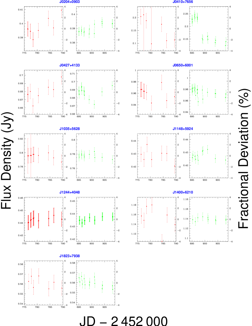
Figure 13: CSO Time Series. The calibrated flux densities for all 9 CSO calibrators are shown as a function of time. Two plots are shown for each CSO. The left-hand plots (red points in the online version) are for 2003 May, and the right-hand plots (green in the online version) are for 2003 September. The horizontal axis indicates the number of days since Julian Date $2\,452\,000$. The vertical axis on the left-hand side of each individual plot shows the flux density of the measurement. The vertical axis on the right-hand side of each plot gives the relative difference from the mean value for the month. The fractional scale is the same for all 9 CSOs. Error-bars show the 1-$\sigma$ uncertainty in the measurements, including random errors and the estimated systematic error. (See the on-line paper for a color version of this figure.)

Figure 13 shows the brightness time series for our fully calibrated CSO data. The data for each CSO are divided into separate plots for May (left) and September (right). All of the plots are shown with the same fractional deviation scale from $-4$% to $+4$% from the mean brightness for each month, as indicated by the right-hand vertical axis of each plot.

The CSO data were analyzed to determine improved amplitude calibrations for the VLA observations. We performed a least squares fit to the CSO data to find the mean brightness of each individual CSO for each month plus multiplicative amplitude corrections for each observing day. The CSO J0410$+$7656 (catalog COINS) was resolved significantly by the VLA, so it was excluded from the least squares fit. No significant variation was seen as a function of elevation angle as shown in Figure 14. This suggests that the elevation gain curves used by the VLA software have properly corrected for elevation effects in the data. Similarly, no trends were seen for hour angle or time of day. Interestingly, the data for individual CSOs appear remarkably stable for measurements made on any single day, as seen in Figure 13 for objects like J0204$+$0903 (catalog COINS), J0650$+$6001 (catalog COINS), and J1035$+$5628 (catalog COINS). These objects show a modest scatter in brightness level from day to day, but within any given day the scatter is typically only a few tenths of a percent. These observations were made many hours apart, with widely varying elevation and azimuth angles and $(u,v)$ coverage, but the measured brightness remains extremely constant, with a sub-day RMS scatter of only 0.5% averaged over all CSOs.

The CSOs show day-to-day variations of a percent or more in amplitude, and there is more scatter present in the May data than is in the September data. We believe that this higher level of variability is not caused by the extreme change in $(u,v)$ coverage, as the high level of scatter can be independently seen in the first three days of observations during May, for which the positions of the antennas are identical. Rather, the higher level of scatter is probably caused by more variable conditions in the atmosphere or ionosphere during 2003 May. Weather conditions during September were generally clear with surface winds calm or less than 3 m s^-1, whereas the May weather was generally overcast with low clouds, winds greater than 5 m s^-1, and a severe thunderstorm on one date. Self-calibration solution intervals as small as 10 seconds were necessary to adequately track phase fluctuations during May, whereas the phase coherence time for September was normally several times longer. The greater phase stability during September leads to more reliable measurements for that month. Results for individual CSOs are shown in Table 9. The mean RMS scatter for CSOs in May was 1.38%, while for September it was only 0.71%. This residual scatter after the least squares adjustment is assumed to indicate the minimum level of uncertainty in the gain calibration of individual objects, and it has been added in quadrature to the noise-induced measurement error determined for each snapshot observation. This total error for the CSOs is shown as 1-$\sigma$ error-bars in Figure 13. The error due to random noise is typically less than 0.1% for the CSO objects, so it generally is negligible relative to the measured amplitude scatter.

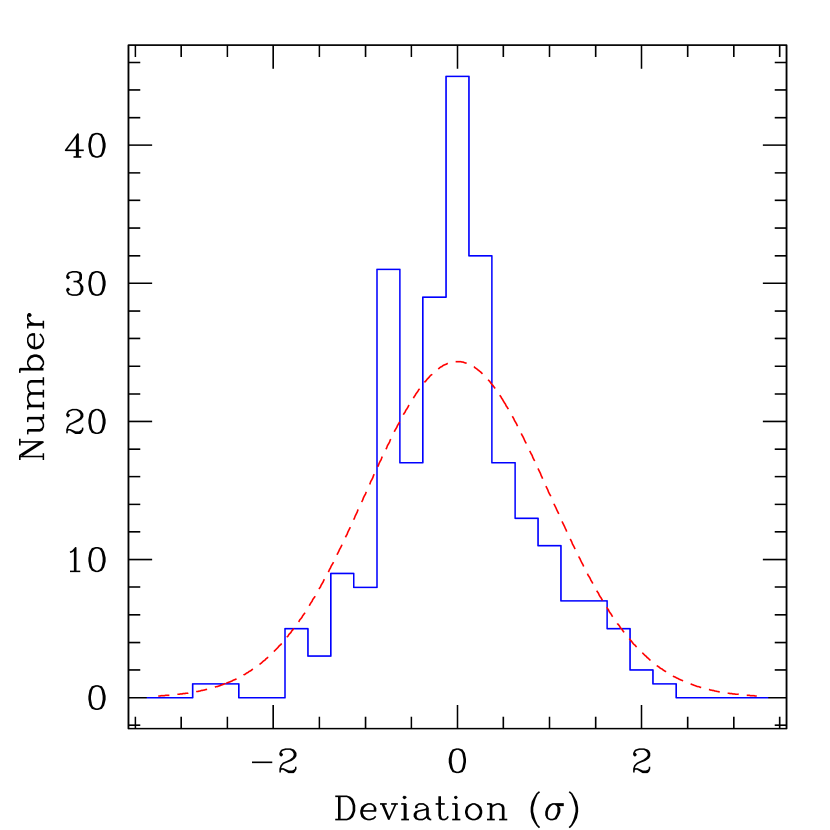
Figure 15: Histogram of the CSO residuals to the calibration fit. The solid (blue) line shows the deviation of each CSO measurement from the least squares calibration fit in units of the RMS scatter for the month of observation, with the May and September data combined. The dashed (red) line shows the corresponding Gaussian (normal) probability function. (See the on-line paper for a color version of this figure.)

Figure 15 shows a histogram of the residuals from the CSO fitting process. Although the profile is not exactly symmetric, the deviations are not dramatically different from a Gaussian distribution. These deviations are probably representative of the deviations to be expected in the galaxy observations.

A.5 Snapshot Imaging

In order to retain as much similarity between the calibrator and target data as possible, the processing steps to extract brightness information from individual snapshots were kept as similar as possible for all objects.

Preliminary imaging of the snapshot data was used to investigate the structure of the sources for use in self-calibration. For those sources which were unresolved, a point source model was used for self-calibration. This model was used for the calibrator sources as well as for several of the target galaxies. For target galaxies with apparent structure, data from multiple snapshot observations were combined (improving $(u,v)$ coverage) to produce a high-fidelity template image of the galaxy using an iterative process of imaging and self-calibration. Then, the clean components from this template image were used as the source model for self-calibration of the individual snapshot observations. For those target galaxies with substantial differences between their May and September appearances (because of a significant change in the core flux level or because of large amounts of extended flux detected in the numerous short baselines in the May data), different templates were used for May and September data.

As a fringe benefit, the self-calibration process was also used to move the core emission of the galaxy to the phase center. Errors in the a priori calibration from the phase calibrator result in images which wobble around from snapshot to snapshot. Self-calibration was used to shift all of the snapshot images to the same apparent position, allowing for easier comparisons between images and reducing measurement scatter resulting from flux falling in different pixel distributions. The scatter in the position of the source peak in the resulting images was generally less than 0.03 pixels for typical sources in our sample.

For target galaxies weaker than 15 mJy, we averaged the two polarizations and two intermediate frequency channels to improve the signal to noise of self-calibration; tests showed a coherence loss less than 0.2% due to this averaging. Solution intervals for target galaxies were kept as short as possible while still providing good fits to the entire snapshot dataset. These solution intervals were around 30 s for most of the galaxies, with the strongest galaxies able to use solution intervals of only 10 s and the weakest galaxy (NGC 777 (catalog NGC)) requiring solution intervals of 4 minutes.

The AIPS task IMAGR was used to produce deconvolved images of our sources using the CLEAN algorithm. All snapshot images were individually examined to verify that there were no significant problems with individual datasets. However, human interaction was eliminated in the final processing stages using a common set of CLEAN parameters to ensure that all snapshot imaging and deconvolution was treated in the same way.

For our variability study, we are only concerned with measuring the flux density in the core of the galaxy, which is unresolved by the VLA. We explored many different schemes to weight data in the $(u,v)$ plane to study the effects of possible extended emission on our measurement of the core flux density. We selected natural weighting to improve sensitivity. Minimum baseline lengths of 0–40 k$\lambda$ were normally sufficient to prevent extended emission from corrupting the core flux density measurement, so we conservatively restricted the $(u,v)$ range for nearly all objects to baselines longer than 100 k$\lambda$, removing sensitivity to regions of emission larger than about 2″. (We used $(u,v)$ ranges of 0–200 k$\lambda$ for J0410$+$7656 (catalog COINS), and 0–400 k$\lambda$ for J1035$+$5628 (catalog VLA_Cal), J1215$+$3448 (catalog VLA_Cal), and J1400$+$6210 (catalog COINS), which have small scale structure resolved by the VLA.) Further concerns regarding the effects of extended emission and jet features on the measurements of the core flux densities are discussed in § 5.

Source flux densities and error estimates were obtained through a combination of methods. The task JMFIT fit a two-dimensional Gaussian to the source core to measure the peak and integrated flux densities. The maximum pixel flux density was recorded as an alternative measure of the peak flux density. (Self-calibration shifted the core to the same pixel position, so this maximum is a reliable estimate of the flux density of the unresolved core.) In addition to error estimates from JMFIT, the noise in each image was measured in a symmetric region surrounding the source. Finally, the task UVFIT was used to fit a point source of fixed location at the phase center of the image to the self-calibrated $(u,v)$ data, as an alternate method of measuring the core flux density. The variability analysis presented in this paper was independently performed on each type of flux density measurement. Although the results varied slightly, no significant differences among measurement techniques were found. For simplicity, we only use the JMFIT peak flux density results in this paper.

The error estimates for the measured brightnesses were modified by adding the mean CSO residual scatter appropriate for the month of observation in quadrature to the random measurement error. For the target galaxies, we also added a 0.5% uncertainty in the gain transfer from the phase calibrators to allow for errors introduced in the time interpolation process and for the spatial extrapolation of the phase calibration from the calibrator to the target positions. We also added an uncertainty ($\sim 1$% for a 5 mJy source) to account for errors introduced by the phase-only self-calibration process (see Cornwell & Fomalont, 1999, equation 10–15). Although this error is insignificant for bright sources such as the phase calibrators, it can be very significant for our weak galaxies with only a few millijanskys of flux density. For the phase calibrators and CSO gain calibrators, only the CSO statistical gain uncertainty was added to the measurement uncertainty.

Appendix B Non-Normal Error Distributions

The statistical analysis made in the main body of our paper, including the $\chi^{2}$ distribution probability and the Monte Carlo simulations, assumed a normal error distribution. The random and systematic errors in our VLA observations are not guaranteed to be normally distributed. However, careful data flagging removed significant outliers in amplitude and phase, eliminating large error sources in the data. Small problems near the noise level do remain in the data, but we believe these to be small and infrequent enough to not cause significant departures from a normal error distribution. Mathematical operations on the interferometry data (such as the conversion of real and imaginary numbers to amplitudes and phases) do not strictly preserve the normal error distribution shape, but we also believe that this effect is not critically important to our results. However, the nature of the systematic errors is not well understood, and significant non-normal errors could possibly have been introduced by such terms.

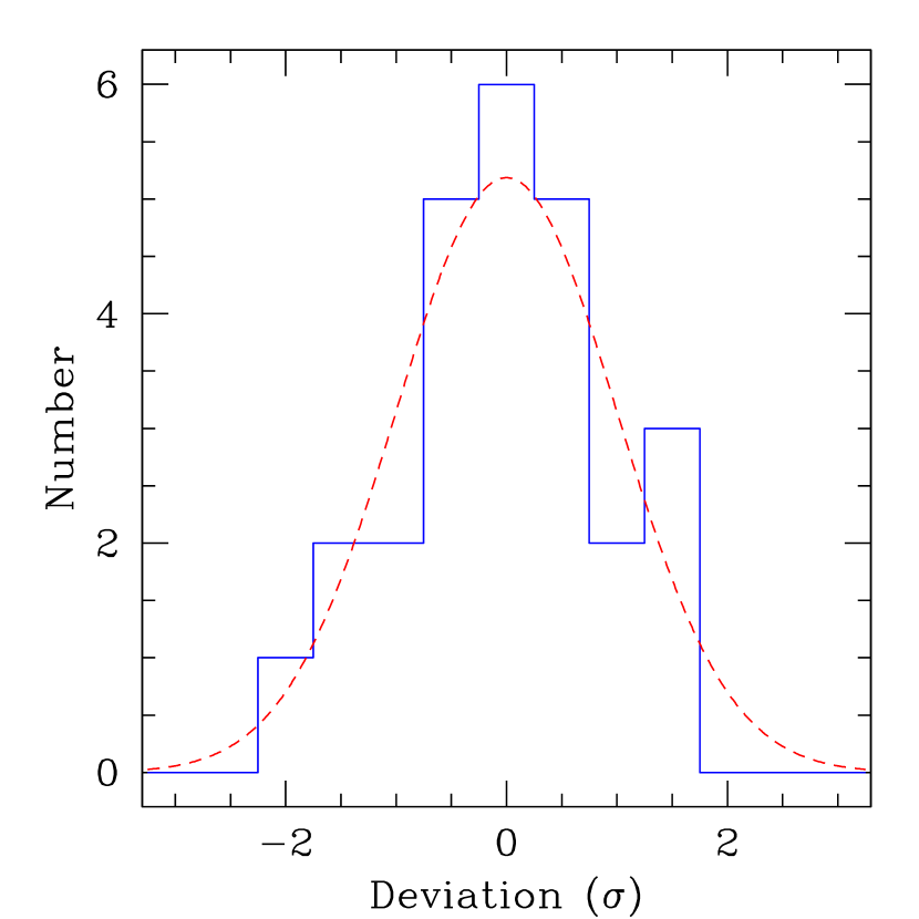
Figure 16: NGC 4168 residual histogram. The solid (blue) line shows a histogram of the residuals for the NGC 4168 measurements assuming a constant flux density, in units of the expected error level. The dashed (red) line shows the corresponding Gaussian (normal) probability function. (See the on-line paper for a color version of this figure.)

We have examined the residual deviations for our galaxies to search for signs of significant deviations from a normal error distribution, but have found none. Figure 16 shows the residual histogram for NGC 4168 (catalog NGC), one of our “constant” galaxies. Given the small number of data-points, a normal distribution agrees relatively well with the measured distribution of errors. Histograms for our other “constant” galaxies show similar results. The distributions are not significantly skewed toward positive or negative errors, and they do not show unexpectedly large numbers of errors at either very large or very small deviations. Sources which we classify as variable tend to have structure functions (§ 5.3) showing larger flux density differences on longer time-scales, and frequently show coherent variations in the time series plots, suggesting that large outliers to the normal error distribution are not responsible for the variability that we detect. We believe that the errors in our galaxy data are reasonably well approximated by a normal error distribution, and are therefore confident that the standard statistical analysis presented in this paper is reasonably accurate.

To investigate the dependence of our Monte Carlo simulations on the exact form of the error distribution, we performed additional simulations using the measured error distribution of NGC 4168 (catalog NGC) and, alternatively, the CSO error distribution (see Figure 15) instead of a normal error distribution. The NGC 4168 (catalog NGC) distribution is similar to the normal distribution, but there are no errors at very large $\sigma$ values because of the small number of data-points. Since NGC 4168 (catalog NGC) is not a strong source, the deviations in its error distribution are probably dominated by the “random” errors in the $(u,v)$ data. The CSO distribution is a composite of many different strong sources, each with different individual scatter levels, and probably gives a better prediction of the possible deviations for the systematic errors.

The suggested brightness temperatures from the alternative error distributions were not substantially different from the normal distribution results. The implied brightness temperatures were generally higher, but only by about $0.1$ dex (a factor of $1.26$) on average for the 50% confidence level calculations. For the 90% confidence level results, about half of the galaxies had implied brightness temperatures increase by less than $0.1$ dex, and about half of the galaxies had increases between $0.2$ and $0.3$ dex (that is, less than a factor of two), with a maximum increase of only $0.33$ dex. The small brightness temperature increases are probably caused by the lack of high-$\sigma$ errors in the NGC 4168 (catalog NGC) and CSO error distributions as the absence of high-$\sigma$ errors requires larger intrinsic changes in brightness to yield the same observed measured flux density changes. These changes are within the $0.3$ dex simulation scatter using different selection criteria as described in § 6.1, and do not significantly change our results.

Appendix C Individual Sources

This CSO is very resolved by our VLA observations. Although following the $(u,v)$ restrictions suggested by the VLA Calibrator Manual results in measurements which are approximately constant with varying hour angle, large changes from day to day with antennas moves prevented this source from being useful as an amplitude calibration tool.

The time series of this CSO during our September run suggests that variability may be present in this object. The $\chi^{2}$ analysis suggests that the probability of seeing the measured scatter is less than 5% for a constant source, and the coherent nature of the variation further supports this. VLBA observations by Peck & Taylor (2000) at 8.4 GHz show that the CSO is dominated by a bright central component with a peak flux density 72% of the flux density measured by our VLA observations, suggesting that variability may indeed be likely in this object.

FT01 found that this CSO had an RMS scatter of $1.3$%, double the scatter of most of the other CSOs in their survey. Our measurements place J1823$+$7938 (catalog COINS) in the middle range of scatter, with two CSOs better and five CSOs worse than J1823$+$7938 (catalog COINS). However, Figure 3 of FT01 shows that J1823$+$7938 (catalog COINS) had extended periods of stability during their long time series, and our short time series may have fortuitously taken place during similar periods of minimal variability.

VLA observations of NGC 777 (catalog NGC) show a point source with position RA $02^{\mathrm{h}}~{}00^{\mathrm{m}}~{}14\fs 907$ Dec $31\arcdeg~{}25\arcmin~{}45\farcs 90$, with an uncertainty of about 25 mas in each dimension. No emission was detected in the VLBA data which was at least $5$-$\sigma$ above the RMS noise level within 200 mas of this position. No object could be identified with imaging performed out to 1″ from this position. Corrected for decoherence, this corresponds to an upper limit of 180 $\mathrm{\mu Jy~{}beam^{-1}}$. Various weighting schemes were applied to the $(u,v)$ data to search for emission on scales up to 6 mas in diameter without success. VLA measurements were made on the day before and the day after the September VLBA observations, but showed rapid variability on the prior day, with peak flux densities varying from $0.7$ to $1.1$ mJy beam^-1. Measurements in 2003 May were as low as $0.5$ mJy beam^-1. We are confident that the variability detected by the VLA is real, and therefore that a compact source with brightness temperature of more than $10^{10}$ K is normally present in this galaxy. We suspect that this LLAGN was simply too weak to be detected by the VLBA during our observing run.

This Seyfert 2 galaxy has a steep spectrum at VLA scales ($\alpha^{5.0}_{8.5}=-0.5$). Our VLBA imaging shows an elongated multiple component structure aligned East-West on the sky. The area shown in Figure 1 contains an integrated flux density of 2.4 mJy, but analysis from running CLEAN suggests that as much as 10 mJy of emission may be present on large scales within 40 mas of the region shown, with the surface brightness lying below the noise level of the image. The peak brightness temperature of $4\times 10^{6}$ K is calculated from the peak flux density value using the area of the synthesized beam. Lal et al. (2004) show results from a 5 GHz VLBI observation made on 1998 February 18. In contrast to our observations, they find only a single, slightly resolved component with a peak of 7.5 mJy beam^-1. It is possible that an outburst has occurred since the Lal et al. observations — in the $\sim 5.6$ years between observations, a jet component traveling at $c$ in the plane of the sky could reach 11 mas from the core, well within the limits from our VLBA image. The VLA flux density changes appear to be correlated with $(u,v)$ changes, and we do not include this object in our short-term variability statistics.

This Seyfert 1.9 galaxy is known to be variable on timescales of several years. Ho & Ulvestad (2001) found a spectral index $\alpha^{1.4}_{5.0}=+0.47$ (1.4 GHz data from 1999 August 29, 5.0 GHz data from 1999 October 31). The Ho & Ulvestad (2001) measurements were significantly brighter than previous measurements, consistent with possible resolution effects and/or variability in the core. NGC 2639 (catalog NGC) was also observed with the VLBA by Wilson et al. (1998) on 1996 May 31 at 1.7, 5.0, and 15 GHz, finding $\alpha^{1.7}_{5.0}=+1.8$ and $\alpha^{5.0}_{15}=-0.04$. These observations found the emission to be unresolved at 1.7 and 5.0 GHz, but somewhat resolved at 15 GHz, with a deconvolved size of $0.70$ mas $\times<0.15$ mas with PA 111°. Our 8.4 GHz results are consistent with a two-component source, with a 34 mJy unresolved core and a 34 mJy resolved component with size $1.94$ mas $\times<0.1$ mas at PA 110°. Taken at face value, this size implies a brightness temperature of at least $10^{9.8}$ K, and suggests that an expanding jet-like feature is present in this galaxy (but is also marginally consistent with our $0.04$ mas² solid angle result). However, the $0.1$ mas upper limit to the width is almost a factor of 20 smaller than the beam width; a more realistic upper limit is $0.5$ mas, which corresponds to a minimum brightness temperature of $10^{9.1}$ K. Lal et al. (2004) show results from a 5 GHz VLBI observation made on 1998 February 18 which also find a slightly resolved source at position angle $\sim 90\arcdeg$. The VLA flux density changes appear to be correlated with $(u,v)$ changes, and we do not include this object in our short-term variability statistics.

Falcke et al. (2000) found a peak flux density of 11.2 mJy beam^-1 in their 5.0 GHz VLBA observations from 1997 June 16. Combined with 15 GHz VLA observations by Nagar et al. (2000) from 1996 October, they calculated a spectral index of $\alpha^{5.0}_{15}=-0.45$. Our 8.4 GHz VLBA measurement is brighter than both of these previous observations. Our observation has a peak to RMS noise ratio of almost 400, but shows no sign of any extended emission. The JMFIT deconvolved size is only about 0.20 mas.

This galaxy is more commonly known as M81 (catalog Messier). The compact VLBA core contains virtually all of the radio flux seen on VLA scales. Bietenholz et al. (1996) and Bietenholz et al. (2000) use these observations to measure the size of the emission region of NGC 3031 (catalog NGC), finding a mean result of $530\pm 100$ $\mu$as $\times$ $180\pm 40$ $\mu$as (at position angle 50°) at 8.4 GHz for their single component model. (The two component model is very similar.) This measurement suggests a brightness temperature of about $10^{10.3}$ K. Given the factor of 5 uncertainty in any individual galaxy, our interstellar scintillation angular size result of about 100 $\mu$as is in remarkably good agreement with their findings. If some fraction of the variability of NGC 3031 (catalog NGC) is intrinsic to the source, this would increase the interstellar scattering size estimate, bringing our value into even closer agreement with Bietenholz et al.

This nearby (3.55 Mpc, Freedman et al., 2001) galaxy has been known to contain a compact, variable radio nucleus for many years. Crane et al. (1976) and de Bruyn et al. (1976) present radio measurements from 1967 to 1975 showing that NGC 3031 (catalog NGC) had varied by up to a factor of $\sim 2$ over that time. Following the SN 1993J (catalog supernova) explosion, the nucleus of NGC 3031 (catalog NGC) was repeatedly observed as part of the SN 1993J (catalog supernova) monitoring campaign, as it was located within the primary beam area of the VLA and VLBA telescopes targeting SN 1993J (catalog supernova). Ho et al. (1999, hereafter H99) present flux densities for NGC 3031 (catalog NGC) at 1.4, 4.9, 8.4, and 15.2 GHz starting 3 days after the supernova explosion and extending to almost 1400 days after the explosion. Since the supernova is located about 170″ away from the nucleus, there is no problem with confusion. However, changing array configurations, uncertainty in the flux density calibrations (CSOs were generally not observed), and other problems cause the uncertainty levels in the individual measurements to be far higher than the measurements presented in this work. Variability statistics are presented in Table 10; a $P_{\chi^{2}}$ analysis gives a probability of only $10^{-13}$ that the nuclear emission was constant. The 8.4 GHz radio light-curves in H99 suggest that NGC 3031 (catalog NGC) has periodic “outbursts” which can double the emission levels, separated by periods of relative “quiet”. The high scatter in Table 10 reflects the strong outburst periods. The observations of NGC 3031 (catalog NGC) presented in this work show far lower variability levels, but are consistent with the “quiet” period scatter levels. Assuming that the variability in H99 is intrinsic, the brightness temperature limits are higher than the values in Table 7, but still consistent with inverse-Compton limits. The 90% confidence estimate to the brightness temperature lower limit is actually consistent with the equipartition brightness temperature limit of $\sim 10^{11}$ K.

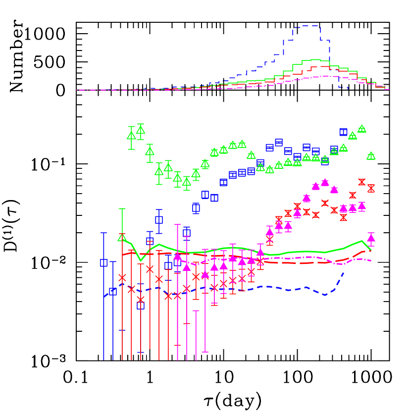
Figure 17: Variability structure functions for NGC 3031 (M81) during 1993–1997. Flux density measurements of NGC 3031 following the supernova 1993J event taken with the VLA and the Ryle Telescope and presented in Ho et al. (1999) have been used to generate structure functions covering time lags from less than one day to 1000 days. The plot information is similar to the plots in Figure 9. Data at 1.4 GHz are shown as solid (magenta) triangles and by the dot-dashed line. Data at 4.9 GHz are shown as (red) crosses and by the long-dashed lines. Data at 8.4 GHz are shown as the open (green) triangles and by the solid lines. Data at 15.2 GHz are shown by the open (blue) squares and by the short-dashed lines. (See the on-line paper for a color version of this figure.)

Figure 17 shows structure function plots for the H99 data. The 1.4 and 4.9 GHz data show no significant intraday variability. The 8.4 GHz data show significant variability down to $\sim 0.5$ days. If the 8.4 GHz data are interpreted in terms of interstellar scintillation, the source angular size predictions from both the initial maximum in the structure function and the de-biased measurement scatter are about 12 $\mu$as at 8.4 GHz. However, we agree with the conclusion by H99 that the large amplitude variations seen in their data are almost certainly intrinsic to NGC 3031 (catalog NGC), as the “outbursts” are visible in all frequencies and are nearly coincident in time. Furthermore, the flux density measurements of SN 1993J (catalog supernova), only 170″ away, show no evidence for large amplitude fluctuations over a period of almost four years. We find it very unlikely that any phase screen covering NGC 3031 (catalog NGC) for this time period would never affect the supernova emission as well. However, the cause of the few percent, “quiet” intraday variability detected in this work could still be either intrinsic or extrinsic to the source itself.

This galaxy contains complicated structure on milliarcsecond scales along with water maser emission. Sawada-Satoh et al. (2000) present VLBA images of this galaxy from 1996 October 20 observations showing a resolved object with multiple components. They found over 18 mJy in three milliarcsecond scale components at $8.4$ GHz, which is far less than the $\sim 120$ mJy we observed on arcsecond scales with the VLA. The VLBI nuclear component has a sharply peaked spectrum, with $\alpha^{8.4}_{15}\approx+0.9$ at low frequencies and $\alpha^{15}_{22}=-1.8$ at high frequencies. Ho & Ulvestad (2001) found a peak spectral index of $\alpha^{1.4}_{4.9}=+0.2$ on arcsecond scales. The VLA scale emission is also extended and shows a small jet feature in our full-$(u,v)$ images. The extended emission in this galaxy did not cause any $(u,v)$ problems, as we found NGC 3079 (catalog NGC) to remain constant with an observed scatter of only $\sim 1$%.

This galaxy was unresolved in the VLBA imaging of Ulvestad & Ho (2001b) and Anderson et al. (2004, hereafter A04).

Falcke et al. (2000) found a peak flux density of 6.2 mJy beam^-1 in their 5.0 GHz VLBA observations from 1997 June 16, while Nagar et al. (2000) found 6.8 mJy beam^-1 in their 15 GHz VLA A-array image. Our VLBA image had a peak of $8.6$ mJy with a peak to RMS noise ratio of $\sim 200$, giving a 3-$\sigma$ upper limit to the size of the unresolved core of 0.65 mas. The variability seen in our VLA observations has some features which correlate with the phase calibrator behavior, and we classify this galaxy as possibly variable.

This LINER 1.9 galaxy was previously observed by Falcke et al. (2000) with the VLBA at 5.0 GHz, finding a peak flux density of 3.5 mJy beam^-1. Our 8.4 GHz VLBA measurement is more than 2 times brighter. Note that our measured VLBA position is almost 0$\farcs$2 north of the position found by Falcke et al. (2000), but is in agreement with our own 8.5 GHz VLA position and is reasonably close to the 15 GHz VLA position of Nagar et al. (2000). The self-calibrated image shows a core-dominated structure with extensions to the East and West. The structure can be modeled as an unresolved core with a peak flux density of 7.9 mJy beam^-1 and an elongated structure 1.5 mas away at PA 74° with a peak flux density of 0.4 mJy beam^-1. Falcke et al. (2000) list a very uncertain position angle of 64°. Thus, all of the emission is contained within a region $1.5$ mas $\times<0.5$ mas in size, corresponding to a brightness temperature of at least $10^{8.3}$ K. Extended emission seen in our full-$(u,v)$ VLA images is removed by our $(u,v)$ weighting, and does not affect our variability measurements.

This Seyfert 1.5 galaxy has the steepest radio spectral index in our galaxy sample, with $\alpha^{1.7}_{5.0}=-0.9$ as measured by Mundell et al. (1995) using MERLIN. Their data show a resolved structure aligned at PA $-10\arcdeg$, with a flux density of 8 mJy at 5 GHz. Although the 5 GHz peak flux density measured by MERLIN was greater than 2 mJy beam^-1, our 8.4 GHz measurements find no detectable emission on VLBI scales. The 5-$\sigma$ upper limit to any compact emission is 260$\mu$Jy beam^-1. Our VLA measurements are severely handicapped by brightness changes caused by $(u,v)$ effects, and we do not include this object in our short-term variability study.

This galaxy appears unresolved in the VLBA imaging of A04, and appears to be constant in our short-term variability analysis.

This galaxy was also essentially unresolved by Ulvestad & Ho (2001b) and A04 in their VLBA imaging. We classify the May VLA measurements as tentative as they have some similarity to the phase calibrator behavior. However, the September observations show a significant decline with time which we believe is reliable.

Essentially unresolved in the VLBA imaging of A04, this galaxy shows modest variability in the September VLA data.

Although essentially unresolved in the VLBA study of A04, this galaxy has about 10 mJy of extended emission in our VLA images, about twice as much as is present in the core. Because of the extensive extended emission, we classify the variability as tentative, although we find no signs of $(u,v)$ effects in the flux variations.

The imaging of this Seyfert 2 galaxy is consistent with an unresolved point source. The source is extended on VLA scales, but the peak flux density in our VLA imaging is similar to the peak flux density in our VLBA image. Variations in our VLA observations appear highly correlated with $(u,v)$ changes, and we do not include this galaxy in our short-term variability analysis.

This Seyfert 1.9 galaxy is relatively weak in our VLBA imaging with a peak of only $1.9$ mJy; self-calibration only partially corrected residual phase errors from the original calibration steps. At most we can only say that the object appears to be compact on VLBI scales. Falcke et al. (2000) found a peak brightness of 3.2 mJy beam^-1 in their 1997 June 16 observations at 5.0 GHz, and 15 GHz VLA A-array imaging by Nagar et al. (2000) found 3.7 mJy beam^-1. Although the September $P_{\chi^{2}}$ value of $0.06$ is above our variability cutoff level, Figure 2c (in the on-line paper) clearly shows variations on a $\sim 4$ day timescale. This is borne out in Figure 9 which shows that the structure function values for time lags of several days are well above the noise level, even if the entire variability does not meet meet our $\chi^{2}$ test.

This galaxy was essentially unresolved by the VLBA study of Ulvestad & Ho (2001b) and A04. We have classified the short-term variability as tentative since the May data could possible have $(u,v)$ effects and the September data could possibly be influenced by the phase calibration.

This galaxy was classified as having a transition nucleus (intermediate between an H II nucleus and a LINER nucleus) by Ho et al. (1997a). Falcke et al. (2000) found a slightly resolved core with a peak flux density of 7.0 mJy beam^-1 and a very uncertain position angle of 11° in their 5.0 GHz VLBA observations. Our 8.4 GHz VLBA observations show a similar result, with a deconvolved core size of about $1.9$ mas $\times<0.2$ mas with a position angle of 12°. Unfortunately, the beam size for our observations was $2.2$ mas $\times 1.0$ mas at PA 6° — nearly aligned with the possible source structure. The galaxy is at high declination, so a full 12^h observing run could better resolve the core. The May short-term variability appears to be reliable. However, the September variability classification effectively depends on the single low point on the second day of observations, and we classify this target-month dataset as tentative.

Figure 1: VLBA 8.4 GHz images of the eight detected LLAGNs are shown as contour plots. Contours start at 2 times the RMS noise level (see Table 3) and increase by factors of 2. Negative contours are indicated by dashed lines. The restoring beam for each image is shown in the bottom left-hand corner of each individual image.

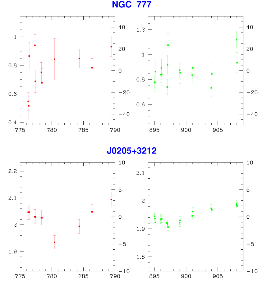
Figure 2: Example target time series for NGC 777. The peak flux density is shown as a function of time, with the left-hand plot of each object (red points) displaying 2003 May data, and the right-hand plot (green points) showing 2003 September data. The corresponding phase calibrator time series is shown immediately below NGC 777. The horizontal axis indicates the number of days since Julian Date $2\,452\,000$. The vertical axis on the left-hand side of each individual plot shows the peak flux density of the measurement, in units of millijanskys per beam for NGC 777 and in units of janskys per beam for the phase calibrator. The vertical axis on the right-hand side of each plot gives the relative difference from the mean value for the month. Error-bars show the 1-$\sigma$ uncertainty in the measurements, including random errors and the estimated systematic errors. (See the on-line paper for color time series plots for all target galaxies.)

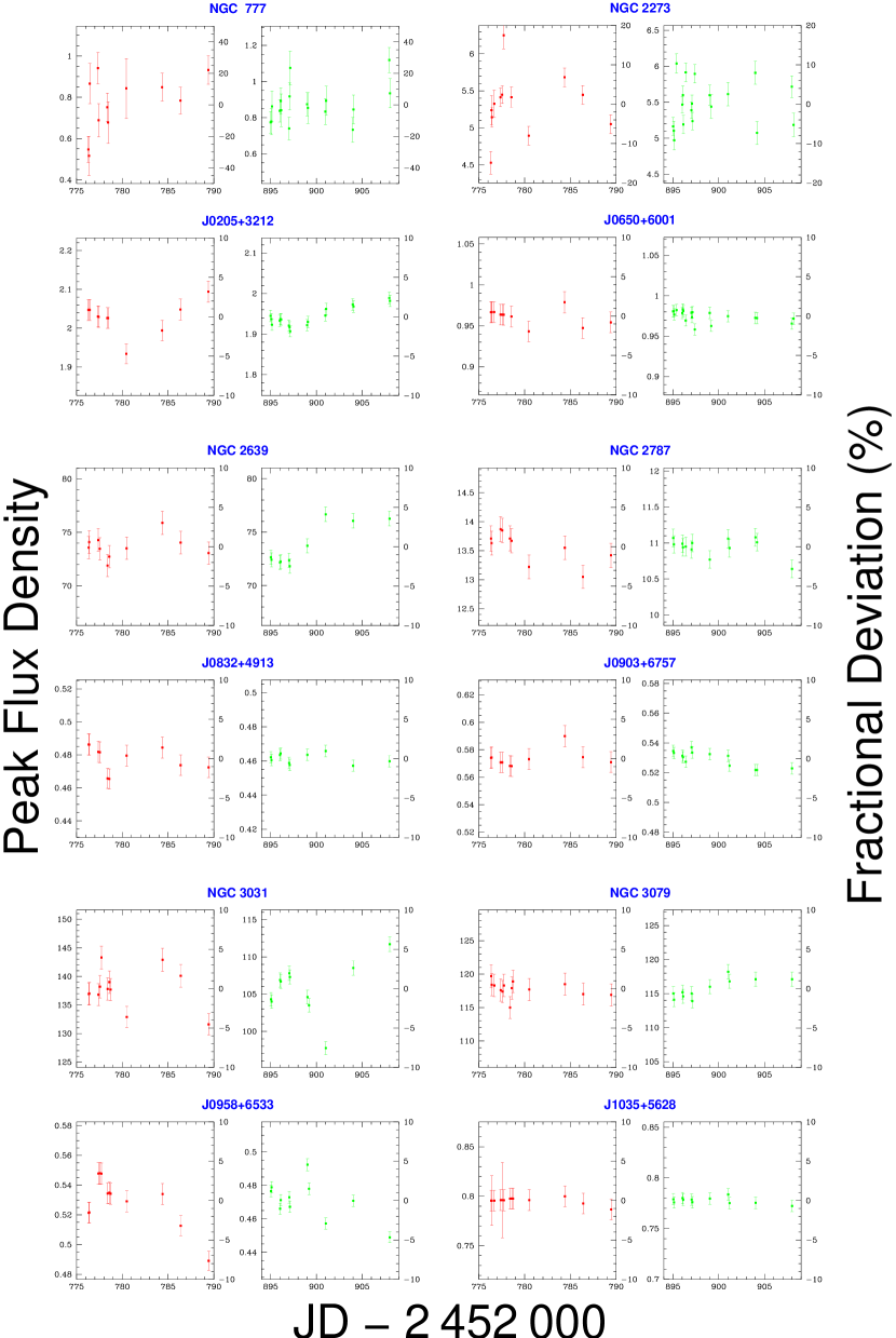
Figure 2a: Target time series for NGC 777, NGC 2273, NGC 2639, NGC 2787, NGC 3031, and NGC 3079. The peak flux density is shown as a function of time for six target galaxies, with the left-hand plot of each object (red points) displaying 2003 May data, and the right-hand plot (green points) showing 2003 September data. For each target galaxy (NGC objects), the corresponding phase calibrator time series is shown immediately below the target plots. The horizontal axis indicates the number of days since Julian Date $2\,452\,000$. The vertical axis on the left-hand side of each individual plot shows the peak flux density of the measurement, in units of millijanskys per beam for the target galaxy and in units of janskys per beam for the phase calibrators. The vertical axis on the right-hand side of each plot gives the relative difference from the mean value for the month. The fractional scale extends from $-10$% to $+10$% for all objects except NGC 777 and NGC 2273. Error-bars show the 1-$\sigma$ uncertainty in the measurements, including random errors and the estimated systematic errors.

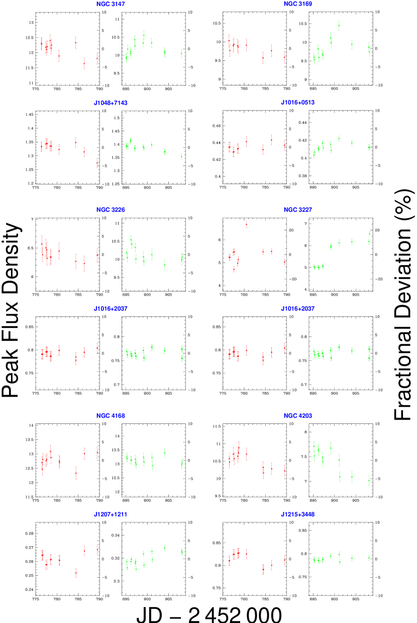
Figure 2b: Target time series for NGC 3147, NGC 3169, NGC 3226, NGC 3227, NGC 4168, and NGC 4203. Details are the same as Figure 2a. The fractional scale extends from $-10$% to $+10$% for all objects except NGC 3227.

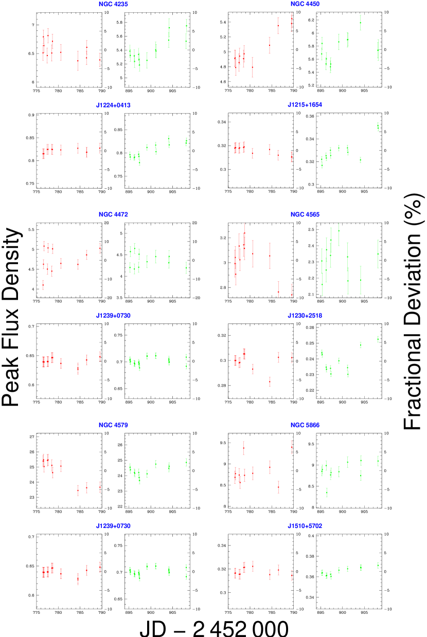
Figure 2c: Target time series for NGC 4235, NGC 4450, NGC 4472, NGC 4565, NGC 4579, and NGC 5866. Details are the same as Figure 2a. The fractional scale extends from $-10$% to $+10$% for all objects except NGC 4472.

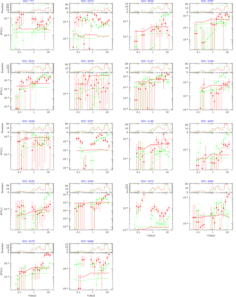
Figure 9: Target galaxy variability structure functions. The first order structure function is plotted for May (red squares) and September (green triangles) as a function of the lag time $\tau$. Error-bars indicate 1-$\sigma$ uncertainty levels. The (mostly) horizontal solid (May, red) and dashed (September, green) lines in the structure function plot areas show the measurement error bias in the structure function, calculated from the estimated uncertainty levels of the individual data-points in each $\tau$ bin. The measured structure functions have not been corrected for the measurement bias. Just above the structure function plot is a histogram of the number of data point comparisons in each structure function point. The May histogram is shown as the solid (red) line, while the September histogram is shown by the dashed (green) line. (See the on-line paper for a color version of this figure.)

Figure 14: The CSO residuals to the calibration fit are plotted as a function of elevation angle. No significant trends are present in the data.

Table 1: Variability Sample

Galaxy	Hubble	AGN Type	RA	Dec	Ref	$M_{\mathrm{BH}}$	Ref	$D$	Ref	$\theta_{1000R_{\mathrm{S}}}$	Phase	Offset
	Type		J2000	J2000		(M☉)		(Mpc)		($\mu$as)	Calibrator	(°)
(1)	(2)	(3)	(4)	(5)	(6)	(7)	(8)	(9)	(10)	(11)	(12)	(13)
NGC 0777 (catalog NGC)	E1	S2/L2::	02 00 14.907	31 25 45.90	1	$8.6\times 10^{8}$	6	66.5	14	255	J0205$+$3212 (catalog VLA_Cal)	1.29
NGC 2273 (catalog NGC)	SB(r)a:	S2	06 50 08.65752	60 50 44.9012	2	$2.0\times 10^{7}$	7	31.6	15	012	J0650$+$6001 (catalog VLA_Cal)	0.82
NGC 2639 (catalog NGC)	(R)SA(r)a?	S1.9	08 43 38.07792	50 12 20.0037	2	$1.1\times 10^{8}$	8	44.4	16	047	J0832$+$4913 (catalog VLA_Cal)	2.07
NGC 2787 (catalog NGC)	SB(r)0$+$	L1.9	09 19 18.60514	69 12 11.6465	2	$1.6\times 10^{8}$	9	07.5	17	433	J0903$+$6757 (catalog VLA_Cal)	1.88
NGC 3031 (catalog NGC)	SA(s)ab	S1.5	09 55 33.1731	69 03 55.061	4	$6.9\times 10^{7}$	6	03.6	18	381	J0958$+$6533 (catalog VLA_Cal)	3.51
NGC 3079 (catalog NGC)	SB(s)c spin	S2	10 01 57.8050	55 40 47.200	5	$4.2\times 10^{7}$	8	17.3	19	048	J1035$+$5628 (catalog VLA_Cal)	4.69
NGC 3147 (catalog NGC)	SA(rs)bc	S2	10 16 53.6503	73 24 02.696	3	$4.4\times 10^{8}$	10	40.9	20	214	J1048$+$7143 (catalog VLA_Cal)	2.89
NGC 3169 (catalog NGC)	SA(s)a pec	L2	10 14 15.05027	03 27 57.8750	2	$7.2\times 10^{7}$	11	40.8	21	035	J1016$+$0513 (catalog VLA_Cal)	1.81
NGC 3226 (catalog NGC)	E2: pec	L1.9	10 23 27.00837	19 53 54.6806	2	$1.4\times 10^{8}$	12	23.6	17	116	J1016$+$2037 (catalog VLA_Cal)	1.74
NGC 3227 (catalog NGC)	SAB(s)a pec	S1.5	10 23 30.579	19 51 54.18	1	$2.2\times 10^{7}$	7	21.1	15	021	J1016$+$2037 (catalog VLA_Cal)	1.76
NGC 4168 (catalog NGC)	E2	S1.9:	12 12 17.2685	13 12 18.701	3	$1.0\times 10^{8}$	6	30.9	17	065	J1207$+$1211 (catalog VLA_Cal)	1.60
NGC 4203 (catalog NGC)	SAB0$-$:	L1.9	12 15 05.0554	33 11 50.382	3	$7.0\times 10^{7}$	9	15.1	17	092	J1215$+$3448 (catalog VLA_Cal)	1.62
NGC 4235 (catalog NGC)	SA(s)a spin	S1.2	12 17 09.8818	07 11 29.670	3	$4.8\times 10^{7}$	13	18.0	22	053	J1222$+$0413 (catalog VLA_Cal)	3.24
NGC 4450 (catalog NGC)	SA(s)ab	L1.9	12 28 29.5908	17 05 05.972	3	$2.1\times 10^{7}$	8	14.1	22	030	J1215$+$1654 (catalog VLA_Cal)	3.21
NGC 4472 (catalog NGC)	E2	S2::	12 29 46.76189	08 00 01.7129	2	$7.2\times 10^{8}$	6	16.3	17	869	J1239$+$0730 (catalog VLA_Cal)	2.44
NGC 4565 (catalog NGC)	SA(s)b? spin	S1.9	12 36 20.78023	25 59 15.6298	2	$2.9\times 10^{7}$	8	17.5	17	032	J1230$+$2518 (catalog VLA_Cal)	1.54
NGC 4579 (catalog NGC)	SAB(rs)b	S1.9/L1.9	12 37 43.5223	11 49 05.488	3	$6.1\times 10^{7}$	6	19.1	22	063	J1239$+$0730 (catalog VLA_Cal)	4.33
NGC 5866 (catalog NGC)	SA0 $+$ spin	T2	15 06 29.49889	55 45 47.5681	2	$5.2\times 10^{7}$	6	15.4	17	067	J1510$+$5702 (catalog VLA_Cal)	1.37

Note. — Column (1) gives the galaxy name. Column (2) gives the Hubble classification and Column (3) AGN classification are from Ho et al. (1997a), with S representing Seyfert galaxies and L representing LINER galaxies. Columns (4) and (5) give the positions of the radio cores of the galaxies (units of right ascension are hours, minutes, and seconds, and units of declination are degrees, arcminutes, and arcseconds), and Column (6) gives the reference for the positions. Our VLA positions should be good to about 0$\farcs$04. Column (7) gives the adopted mass of the central black hole, using velocity dispersion measurements taken from the references in Column (8) and the $M_{\mathrm{BH}}$-$\sigma$ relation from Tremaine et al. (2002). Columns (9) and (10) give the adopted distance and reference for each galaxy. For cases in which only recession velocities are known, we adopt a value of $H_{0}=75$ km s^-1 Mpc^-1. Column (11) gives the angular size in microarcseconds equivalent to 1000 Schwarzschild radii at the distance of the galaxy. Column (12) gives the phase calibrator used for our VLA variability study, and Column (13) gives the angular separation between the galaxy and the calibrator.

References. — 1. 8.5 GHz VLA observations, this paper; 2. 8.4 GHz VLBA observations, this paper; 3. ICRF Ma et al. 1998 (see the extension at ftp://hpiers.obspm.fr/iers/icrf/iau/icrf-Ext.1/); 4. Trotter et al. 1998, Fig. 4; 5. Anderson et al. 2004; 6. Prugniel et al. 2001 (see the HyperLeda database at http://www-obs.univ-lyon1.fr/hypercat/); 7. Nelson & Whittle 1995; 8. McElroy 1995; 9. Barth, Ho, & Sargent 2002; 10. Whitmore, McElroy, & Tonry 1985; 11. Héraudeau & Simien 1998; 12. Simien & Prugniel 2002; 13. Jiménez-Benito et al. 2000; 14. de Vaucouleurs et al. 1991; 15 Terry et al. 2002; 16. Gallimore et al. 1999; 17. Tonry et al. 2001; 18. Freedman et al. 2001; 19. Tully et al. 1992; 20. Tully 1988; 21. Tutui & Sofue 1997; 22. Solanes et al. 2002

Table 2: VLBA Observation Details

Galaxy	UT Date	Phase	Offset	Check
		Calibrator	(°)	(°)
(1)	(2)	(3)	(4)	(5)
NGC 0777 (catalog NGC)	2003 Sep 15	J0205+3212 (catalog ICRF)	1.29	1.54
NGC 2273 (catalog NGC)	2003 Sep 25	J0650+6001 (catalog VLBA)	0.82	1.64
NGC 2639 (catalog NGC)	2003 Mar 03	J0832+4913 (catalog ICRF)	2.07	3.16
NGC 2787 (catalog NGC)	2003 Mar 03	J0903+6757 (catalog VLBA)	1.88	1.14
NGC 3169 (catalog NGC)	2003 Mar 03	J1016+0513 (catalog VLBA)	1.81	2.30
NGC 3226 (catalog NGC)	2003 Oct 02	J1024+1912 (catalog ICRF)	0.76	2.36
NGC 3227 (catalog NGC)	2003 Oct 02	J1024+1912 (catalog ICRF)	0.72	2.36
NGC 4472 (catalog NGC)	2003 Sep 22	J1238+0723 (catalog VLBA)	2.14	2.70
NGC 4565 (catalog NGC)	2003 Sep 25	J1230+2518 (catalog VLBA)	1.54	3.52
NGC 5866 (catalog NGC)	2003 Mar 25	J1510+5702 (catalog ICRF)	1.37	5.77

Note. — Column (1): Galaxy name. Column (2): UT observing date. Column (3): Calibration source for phase referencing. Column (4): Angular separation between the galaxy and phase calibrator. Column (5): Angular separation between the phase calibrator and the check source.

Table 3: VLBA Galaxy Attributes

Galaxy	$S^{\mathrm{P}}_{\nu}$	$S^{\mathrm{I}}_{\nu}$	RMS	coherence	$\Theta_{\mathrm{min}}$	$\Theta_{\mathrm{max}}$	$T_{\mathrm{b}}$
	($\mathrm{mJy~{}beam^{-1}}$)	(mJy)	($\mathrm{\mu Jy~{}beam^{-1}}$)	ratio	(mas)	(mas)	(K)
(1)	(2)	(3)	(4)	(5)	(6)	(7)	(8)
NGC 0777 (catalog NGC)	$\cdots$	$\cdots$	30	1.185	$\cdots$	$\cdots$	$\cdots$
NGC 2273 (catalog NGC)	$0.44\pm 0.04$	$2.4\pm 0.2$	31	1.020	$\cdots$	$\cdots$	$\phantom{string}4\times 10^{6}$
NGC 2639 (catalog NGC)	$53\pm 3$	$66\pm 3$	50	1.014	$\cdots$	$\cdots$	$>1\times 10^{9}$
NGC 2787 (catalog NGC)	$14.4\pm 0.7$	$14.4\pm 0.7$	37	1.005	0.15	0.23	$>1\times 10^{9}$
NGC 3169 (catalog NGC)	$8.6\pm 0.4$	$8.9\pm 0.5$	38	1.005	0.33	0.49	$>5\times 10^{8}$
NGC 3226 (catalog NGC)	$7.9\pm 0.4$	$9.8\pm 0.5$	37	1.006	$\cdots$	$\cdots$	$>2\times 10^{8}$
NGC 3227 (catalog NGC)	$\cdots$	$\cdots$	42	1.219	$\cdots$	$\cdots$	$\cdots$
NGC 4472 (catalog NGC)	$3.6\pm 0.2$	$3.8\pm 0.2$	32	1.098	0.00	0.73	$>2\times 10^{8}$
NGC 4565 (catalog NGC)	$1.9\pm 0.1$	$1.9\pm 0.1$	36	1.062	0.54	0.86	$>1\times 10^{8}$
NGC 5866 (catalog NGC)	$5.4\pm 0.3$	$7.1\pm 0.4$	40	1.007	1.92	1.99	$>1\times 10^{8}$

Note. — Column (1) gives the galaxy name. Column (2) gives the peak flux density of the source from Gaussian fitting, corrected for decoherence, while Column (3) gives the integrated flux density in the VLBA image. Column (4) gives the RMS noise in the image far away from the source. Column (5) gives the estimated increase in peak flux density by correcting for coherence losses based on self-calibration improvements in the check source. Columns (6) and (7) give respectively the 1-$\sigma$ lower and upper limits on the deconvolved major axis of the source sized obtained through Gaussian fitting of the image. Column (8) gives the lower limit to the brightness temperature. For galaxies with no deconvolved size listed in Column (7), details of the calculation procedure are given in Appendix C. For the remaining galaxies, a beam size of the maximum of Column (7) or one third of the synthesized beam width in both major and minor axes was assumed, since source sizes significantly smaller than the synthesized beam are unreliable even for our images with signal to noise ratios of several hundred.

Table 4: VLA Observation Details

UT Date	LST Start	LST End	Length
(1)	(2)	(3)	(4)
D$\rightarrow$A Configuration
May 16	3:00	14:30	11.5
May 17	4:30	14:30	10.0
May 18	5:00	15:00	10.0
May 20	7:00	12:00	5.0
May 24	5:00	10:00	5.0
May 26	5:00	10:00	5.0
May 29	6:30	11:30	5.0
A$\rightarrow$BnA Configuration
Sep 12	4:00	14:00	10.0
Sep 13	4:00	14:00	10.0
Sep 14	4:00	14:30	10.5
Sep 16	4:00	10:30	6.5
Sep 18	4:00	10:30	6.5
Sep 21	4:00	10:30	6.5
Sep 25	4:00	10:30	6.5

Note. — Column (1): UT observing date. Column (2) is the Local Sidereal Time (LST) at the start of observations, and Column (3) is the LST at the end of observations in hours and minutes. Column (4) gives the total observing time in hours for the corresponding day.

Table 5: Variability Statistics

		2003 May							2003 September
Name	Class	$N$	$<S_{\nu}>$	$\sigma_{\mathrm{e}}$	$\sigma_{\mathrm{s}}$	$\sigma_{\mathrm{d}}$	$P_{\chi^{2}}$		$N$	$<S_{\nu}>$	$\sigma_{\mathrm{e}}$	$\sigma_{\mathrm{s}}$	$\sigma_{\mathrm{d}}$	$P_{\chi^{2}}$	$F$	$\delta F$
			(Jy bm-1)	(%)	(%)	(%)				(Jy bm-1)	(%)	(%)	(%)		(%)	(%)
(1)	(2)	(3)	(4)	(5)	(6)	(7)	(8)		(9)	(10)	(11)	(12)	(13)	(14)	(15)	(16)
Target Galaxies and Phase Calibrators
NGC 0777 (catalog NGC)	P	11	0.00076	11.4	18.8	14.9	$1.4\times 10^{-4}$		17	0.00087	8.7	11.8	8.0	$9.4\times 10^{-3}$	+0.3	6.3
J0205$+$3212 (catalog VLA_Cal)	C	11	2.03	1.4	2.0	1.4	$2.0\times 10^{-2}$		17	1.943	0.7	1.2	1.0	$5.6\times 10^{-5}$	-5.9	1.4
NGC 2273 (catalog NGC)	E	12	0.0053	2.8	7.9	7.4	$1.1\times 10^{-12}$		19	0.00547	2.5	5.9	5.3	$2.0\times 10^{-13}$	+1.1	3.9
J0650$+$6001 (catalog VLA_Cal)	CS	12	0.962	1.4	1.0	$\cdots$	$8.8\times 10^{-1}$		19	0.975	0.7	0.7	0.0	$4.4\times 10^{-1}$	+1.7	1.0
NGC 2639 (catalog NGC)	J	10	0.0737	1.5	1.4	$\cdots$	$5.0\times 10^{-1}$		10	0.0736	0.9	2.6	2.5	$1.9\times 10^{-12}$	-2.8	1.2
J0832$+$4913 (catalog VLA_Cal)	C	10	0.478	1.4	1.7	0.9	$1.5\times 10^{-1}$		10	0.4613	0.7	0.6	$\cdots$	$5.9\times 10^{-1}$	-3.3	0.8
NGC 2787 (catalog NGC)	P	10	0.01357	1.6	2.0	1.1	$1.1\times 10^{-1}$		13	0.01095	1.1	1.1	0.2	$4.1\times 10^{-1}$	-19.4	1.2
J0903$+$6757 (catalog VLA_Cal)	C	10	0.574	1.4	1.1	$\cdots$	$8.0\times 10^{-1}$		13	0.529	0.7	1.0	0.7	$3.3\times 10^{-2}$	-8.3	1.0
NGC 3031 (catalog NGC)	P	12	0.1379	1.5	2.5	2.0	$8.7\times 10^{-4}$		11	0.106	0.9	3.4	3.3	$2.5\times 10^{-28}$	-26.2	2.5
J0958$+$6533 (catalog VLA_Cal)	C	12	0.530	1.4	3.2	2.9	$2.0\times 10^{-9}$		11	0.471	0.7	2.4	2.3	$1.2\times 10^{-20}$	-8.1	2.6
NGC 3079 (catalog NGC)	EJ	13	0.1178	1.5	1.0	$\cdots$	$9.5\times 10^{-1}$		11	0.1157	0.9	1.2	0.8	$4.2\times 10^{-2}$	-2.4	0.9
J1035$+$5628 (catalog VLA_Cal)	CS	13	0.7956	2.0	0.4	$\cdots$	$1.0\times 10^{0}$		11	0.7776	0.7	0.4	$\cdots$	$9.8\times 10^{-1}$	-1.9	0.8
NGC 3147 (catalog NGC)	D	12	0.01213	1.6	1.9	1.0	$1.4\times 10^{-1}$		13	0.01018	1.2	1.9	1.5	$1.4\times 10^{-3}$	-16.3	1.8
J1048$+$7143 (catalog VLA_Cal)	C	12	1.330	1.4	1.5	0.6	$2.4\times 10^{-1}$		13	1.388	0.7	1.2	0.9	$9.3\times 10^{-4}$	+6.2	1.6
NGC 3169 (catalog NGC)	D	10	0.00982	1.7	1.5	$\cdots$	$6.0\times 10^{-1}$		12	0.00983	1.2	2.7	2.4	$4.4\times 10^{-7}$	+0.1	1.1
J1016$+$0513 (catalog VLA_Cal)	C	10	0.435	1.4	1.1	$\cdots$	$7.8\times 10^{-1}$		12	0.412	0.7	1.2	1.0	$6.7\times 10^{-4}$	-6.5	0.9
NGC 3226 (catalog NGC)	E	11	0.00639	2.1	1.6	$\cdots$	$8.6\times 10^{-1}$		12	0.01013	1.3	2.0	1.5	$2.0\times 10^{-3}$	+47.9	1.4
J1016$+$2037 (catalog VLA_Cal)	C	22	0.793	1.4	0.8	$\cdots$	$1.0\times 10^{0}$		24	0.765	0.7	0.9	0.6	$1.3\times 10^{-2}$	-3.9	0.6
NGC 3227 (catalog NGC)	EJ	11	0.0054	2.3	9.4	9.1	$2.0\times 10^{-25}$		12	0.0056	2.0	10.9	10.7	$8.4\times 10^{-69}$	-6.0	3.0
J1016$+$2037 (catalog VLA_Cal)	C	22	0.793	1.4	0.8	$\cdots$	$1.0\times 10^{0}$		24	0.765	0.7	0.9	0.6	$1.3\times 10^{-2}$	-3.9	0.6
NGC 4168 (catalog NGC)	P	12	0.01278	1.6	1.8	0.6	$3.6\times 10^{-1}$		14	0.01313	1.1	1.0	$\cdots$	$6.8\times 10^{-1}$	+2.6	1.9
J1207$+$1211 (catalog VLA_Cal)	C	12	0.262	1.4	1.8	1.1	$7.6\times 10^{-2}$		14	0.319	0.7	1.8	1.6	$5.4\times 10^{-12}$	+18.3	2.1
NGC 4203 (catalog NGC)	P	12	0.01052	1.7	2.2	1.4	$5.1\times 10^{-2}$		11	0.00743	1.4	3.4	3.1	$8.4\times 10^{-9}$	-30.1	1.0
J1215$+$3448 (catalog VLA_Cal)	C	12	0.814	1.4	1.7	1.0	$9.4\times 10^{-2}$		11	0.789	0.7	0.6	$\cdots$	$7.2\times 10^{-1}$	-1.5	0.7
NGC 4235 (catalog NGC)	P	12	0.00656	2.0	2.3	1.0	$2.0\times 10^{-1}$		14	0.00540	1.8	3.2	2.7	$1.5\times 10^{-4}$	-19.7	1.2
J1222$+$0413 (catalog VLA_Cal)	C	12	0.822	1.4	0.6	$\cdots$	$1.0\times 10^{0}$		14	0.805	0.7	2.0	1.8	$2.9\times 10^{-15}$	-3.9	0.7
NGC 4450 (catalog NGC)	EJ	12	0.00503	2.3	4.6	4.0	$5.3\times 10^{-6}$		12	0.00575	1.9	3.4	2.9	$1.8\times 10^{-5}$	+5.4	1.8
J1215$+$1654 (catalog VLA_Cal)	C	12	0.3159	1.4	1.0	$\cdots$	$8.4\times 10^{-1}$		12	0.330	0.7	3.3	3.2	$1.1\times 10^{-39}$	+3.6	0.9
NGC 4472 (catalog NGC)	E	11	0.00473	2.6	6.5	6.0	$1.2\times 10^{-10}$		11	0.00437	2.9	3.9	2.6	$3.1\times 10^{-2}$	-9.8	3.1
J1239$+$0730 (catalog VLA_Cal)	C	22	0.641	1.4	0.9	$\cdots$	$9.9\times 10^{-1}$		23	0.701	0.7	0.9	0.5	$4.1\times 10^{-2}$	+8.8	0.6
NGC 4565 (catalog NGC)	P	12	0.00302	3.1	5.0	3.8	$1.0\times 10^{-3}$		11	0.00231	3.4	4.6	3.0	$6.1\times 10^{-2}$	-21.0	3.9
J1230$+$2518 (catalog VLA_Cal)	C	12	0.299	1.4	2.1	1.6	$4.6\times 10^{-3}$		11	0.239	0.7	3.1	3.1	$1.4\times 10^{-34}$	-22.3	2.3
NGC 4579 (catalog NGC)	D	11	0.0248	1.5	3.2	2.9	$5.7\times 10^{-7}$		12	0.0243	0.9	1.4	1.1	$6.4\times 10^{-3}$	+2.4	1.0
J1239$+$0730 (catalog VLA_Cal)	C	22	0.641	1.4	0.9	$\cdots$	$9.9\times 10^{-1}$		23	0.701	0.7	0.9	0.5	$4.1\times 10^{-2}$	+8.8	0.6
NGC 5866 (catalog NGC)	P	10	0.00884	1.7	3.5	3.1	$2.9\times 10^{-5}$		11	0.00887	1.3	2.4	2.1	$2.1\times 10^{-5}$	-1.6	3.2
J1510$+$5702 (catalog VLA_Cal)	C	10	0.3179	1.4	0.9	$\cdots$	$9.1\times 10^{-1}$		11	0.365	0.7	1.0	0.7	$3.1\times 10^{-2}$	+13.5	0.8
CSO Calibrators
J0204$+$0903 (catalog COINS)	S	11	0.396	1.4	1.5	0.6	$2.9\times 10^{-1}$		14	0.3898	0.7	0.8	0.3	$2.6\times 10^{-1}$	-3.9	0.9
J0410$+$7656 (catalog COINS)	SE	7	2.16	7.8	2.2	$\cdots$	$1.9\times 10^{-1}$		17	2.19	0.7	2.1	2.0	$2.4\times 10^{-22}$	+4.6	1.0
J0427$+$4133 (catalog COINS)	S	9	0.679	1.4	1.4	0.2	$4.2\times 10^{-1}$		13	0.687	0.7	0.9	0.6	$4.5\times 10^{-2}$	+0.0	0.8
J0650$+$6001 (catalog COINS)	CS	12	0.962	1.4	1.0	$\cdots$	$8.8\times 10^{-1}$		19	0.975	0.7	0.7	0.0	$4.4\times 10^{-1}$	+1.7	1.0
J1035$+$5628 (catalog COINS)	CS	13	0.7956	2.0	0.4	$\cdots$	$1.0\times 10^{0}$		11	0.7776	0.7	0.4	$\cdots$	$9.8\times 10^{-1}$	-1.9	0.8
J1148$+$5924 (catalog COINS)	S	7	0.428	1.4	1.2	$\cdots$	$5.8\times 10^{-1}$		11	0.4274	0.7	0.7	$\cdots$	$4.7\times 10^{-1}$	-0.2	0.8
J1244$+$4048 (catalog COINS)	S	44	0.4428	1.4	0.4	$\cdots$	$1.0\times 10^{0}$		42	0.4356	0.7	0.4	$\cdots$	$1.0\times 10^{0}$	-2.3	0.4
J1400$+$6210 (catalog COINS)	S	7	1.152	1.4	2.2	1.8	$1.1\times 10^{-2}$		10	1.1387	0.7	0.3	$\cdots$	$1.0\times 10^{0}$	+0.3	1.5
J1823$+$7938 (catalog COINS)	S	7	0.561	1.4	1.0	$\cdots$	$8.0\times 10^{-1}$		14	0.560	0.7	0.7	0.2	$3.6\times 10^{-1}$	+0.8	0.8

Note. — Simple variability statistics are given for the target galaxies and calibration sources in this study. Column (1) gives the name of the object. The phase calibrator used for each target galaxy is listed immediately below the target information, so some calibrators are listed multiple times. Column (2) gives the object classification. P indicates a point source, D indicates a galaxy dominated by a point source containing at least 80% of the flux, E indicates an extended source, and J indicates the presence of a jet feature. C indicates that the source was used as a phase calibrator, and S indicates that the object is a CSO. Columns (3) and (9) give the number of independent observations for May and September, respectively. Columns (4) and (10) give the mean peak flux density. Columns (5) and (11) give the mean expected scatter in the data based on the measurement noise and expected statistical errors. Columns (6) and (12) give the actual RMS scatter of the data. Columns (7) and (13) give the predicted de-biased scatter in the data, correcting for measurement uncertainty. Columns (8) and (14) give the $\chi^{2}$ probability that a constant brightness object would have an RMS scatter at least as large as actually observed given the expected measurement errors for the given number of data-points ($N-1$ degrees of freedom). Column (15) gives the fractional variation from May to September, and Column (16) gives the uncertainty in that value. The fractional variation was calculated from the mean of the last three days of May and the first three days of September in order to provide the most similar $(u,v)$ coverage. See § 5.1 and § 7 for more details.

Table 6: Galaxy Variability Fractions

	Reliable			Reliable $+$ Tentative
Class	Number	Fraction		Number	Fraction
		(%)			(%)
(1)	(2)	(3)		(4)	(5)
Galaxies with $P_{\chi^{2}}<0.01$
E$+$J	$1/\phantom{0}4$	$25\pm 22$		$3/\phantom{0}6$	$50\pm 20$
D	$1/\phantom{0}2$	$50\pm 35$		$4/\phantom{0}6$	$67\pm 19$
P	$8/14$	$57\pm 13$		$9/16$	$56\pm 12$
P$+$D	$9/16$	$56\pm 12$		$13/22$	$59\pm 10$
P$+$D$+$E$+$J	$10/20$	$50\pm 11$		$16/28$	$57\pm\phantom{0}9$
Galaxies with $P_{\chi^{2}}<0.001$
P$+$D$+$E$+$J	$7/20$	$35\pm 11$		$12/28$	$43\pm\phantom{0}9$
Galaxies with $P_{\chi^{2}}<0.0005$
P$+$D$+$E$+$J	$5/20$	$25\pm 10$		$10/28$	$36\pm\phantom{0}9$
Galaxies with $P_{\chi^{2}}<0.01$ and $\sigma_{\mathrm{s}}>4$%
P$+$D$+$E$+$J	$3/20$	$15\pm\phantom{0}8$		$4/28$	$14\pm\phantom{0}7$
Galaxies with $P_{\chi^{2}}<0.01$ and $\sigma_{\mathrm{d}}>4$%
P$+$D$+$E$+$J	$2/20$	$10\pm\phantom{0}7$		$3/28$	$11\pm\phantom{0}6$

Note. — Column (1) indicates the object classes studied, using the classification from § 5.1. Columns (2) and (4) give the number counts for the number of variable sources and the total number of sources. Columns (3) and (5) give the fraction of source-months which show variability. Columns (2) and (3) give information for only datasets classified as “reliable”, while Columns (4) and (5) also include “tentative” datasets. The galaxies with known $(u,v)$ problems (NGC 2273, NGC 2639, NGC 3227, and NGC 4472) are not included in these statistics.

Table 7: Variability Categorization

Galaxy	Class	Var.	$T_{\mathrm{b,O,1}}$	$T_{\mathrm{b,O,4}}$	$T_{\mathrm{b,M,50}}$	$T_{\mathrm{b,M,90}}$	$T_{\mathrm{b,R,50}}$	$T_{\mathrm{b,R,90}}$
			($\log_{10}(K)$)	($\log_{10}(K)$)	($\log_{10}(K)$)	($\log_{10}(K)$)	($\log_{10}(K)$)	($\log_{10}(K)$)
(1)	(2)	(3)	(4)	(5)	(6)	(7)	(8)	(9)
NGC 0777 (catalog NGC)	P	var	13.7	11.6	10.0	9.8	10.8	10.0
NGC 2787 (catalog NGC)	P	const	8.5	7.5	7.6	$\cdots$	7.9	$\cdots$
NGC 3031 (catalog NGC)	P	var	11.2	9.5	9.1	8.9	9.5	9.3
NGC 3079 (catalog NGC)	EJ	const	10.2	7.4	$\cdots$	$\cdots$	$\cdots$	$\cdots$
NGC 3147 (catalog NGC)	D	var	10.8	10.3	9.9	9.8	10.3	10.0
NGC 3169 (catalog NGC)	D	var?	10.7	10.4	10.1	9.9	10.5	10.2
NGC 3226 (catalog NGC)	E	var	10.9	9.8	9.3	8.9	9.8	9.1
NGC 4168 (catalog NGC)	P	const	7.2	7.1	$\cdots$	$\cdots$	$\cdots$	$\cdots$
NGC 4203 (catalog NGC)	P	var?	9.8	9.0	8.8	8.4	9.1	8.7
NGC 4235 (catalog NGC)	P	var	9.1	8.7	8.5	8.2	8.7	8.4
NGC 4450 (catalog NGC)	EJ	var?	9.6	9.0	8.9	8.4	9.1	8.9
NGC 4565 (catalog NGC)	P	var	9.7	9.2	8.8	8.4	9.2	8.6
NGC 4579 (catalog NGC)	D	var?	10.1	9.7	9.4	9.0	9.8	9.3
NGC 5866 (catalog NGC)	P	var?	12.4	10.5	9.5	9.3	12.2	10.4

Note. — Column (1) gives the galaxy name. Column (2) gives the image classification from Table 5. Column (3) gives our variability classification for the target galaxy; “const” indicates that the source appears to be constant, and “var” indicates that the source is variable. Galaxies which have slightly questionable variability are designated by “var?”. Columns (4) and (5) give the highest and fourth highest apparent brightness temperatures measured directly from the target dataset. Columns (6) and (7) give the 50% (best) and 90% (minimum) confidence estimates of the variability brightness temperature, respectively, for our first Monte Carlo simulation. Columns (8) and (9) give the results for the random brightness temperature simulation, which is our best attempt to account for all biases. See § 6.1 for details.

Table 8: Intraday Scintillation Results

				2003 May								2003 September
Galaxy	$\nu_{0}$	$\theta_{\mathrm{F}}$	$t_{\mathrm{F}}$	$\tau_{\mathrm{max}}$	$\theta_{\tau}$	$m$	$\theta_{m}$	$R$	$T_{\mathrm{b}\,m}$	$\tau_{m}$		$\tau_{\mathrm{max}}$	$\theta_{\tau}$	$m$	$\theta_{m}$	$R$	$T_{\mathrm{b}\,m}$	$\tau_{m}$
	(GHz)	($\mu$as)	(day)	(day)	($\mu$as)	(%)	($\mu$as)	($R_{\mathrm{S}}$)	($\log_{10}(K)$)	(day)		(day)	($\mu$as)	(%)	($\mu$as)	($R_{\mathrm{S}}$)	($\log_{10}(K)$)	(day)
(1)	(2)	(3)	(4)	(5)	(6)	(7)	(8)	(9)	(10)	(11)		(12)	(13)	(14)	(15)	(16)	(17)	(18)
NGC 0777 (catalog NGC)	11.2	2.7	0.12	0.5	11	14.9	19	38	10.6	0.9		0.13	3	8.0	33	65	10.2	1.5
NGC 2787 (catalog NGC)	9.8	3.0	0.14	$\cdots$	$\cdots$	$\cdots$	$\cdots$	$\cdots$	$\cdots$	$\cdots$		$\cdots$	$\cdots$	$\cdots$	$\cdots$	$\cdots$	$\cdots$	$\cdots$
NGC 3031 (catalog NGC)	9.4	3.1	0.14	0.4	9	2.0	101	130	11.4	4.5		6	133	3.3	66	86	11.7	3.0
NGC 3079 (catalog NGC)	8.8	3.4	0.14	$\cdots$	$\cdots$	$\cdots$	$\cdots$	$\cdots$	$\cdots$	$\cdots$		$\cdots$	$\cdots$	$\cdots$	$\cdots$	$\cdots$	$\cdots$	$\cdots$
NGC 3147 (catalog NGC)	9.5	3.0	0.14	$\cdots$	$\cdots$	$\cdots$	$\cdots$	$\cdots$	$\cdots$	$\cdots$		3	64	1.5	126	300	10.1	5.9
NGC 3169 (catalog NGC)	9.1	3.2	0.14	$\cdots$	$\cdots$	$\cdots$	$\cdots$	$\cdots$	$\cdots$	$\cdots$		6.5	149	2.4	86	1200	10.4	3.7
NGC 3226 (catalog NGC)	8.5	3.6	0.15	$\cdots$	$\cdots$	$\cdots$	$\cdots$	$\cdots$	$\cdots$	$\cdots$		1.0	24	1.5	132	570	10.0	5.5
NGC 4168 (catalog NGC)	7.5	3.5	0.18	$\cdots$	$\cdots$	$\cdots$	$\cdots$	$\cdots$	$\cdots$	$\cdots$		$\cdots$	$\cdots$	$\cdots$	$\cdots$	$\cdots$	$\cdots$	$\cdots$
NGC 4203 (catalog NGC)	6.4	3.1	0.28	$\cdots$	$\cdots$	$\cdots$	$\cdots$	$\cdots$	$\cdots$	$\cdots$		$\geq 10$	$\geq 111$	3.1	43	440	10.9	3.9
NGC 4235 (catalog NGC)	7.7	3.5	0.17	$\cdots$	$\cdots$	$\cdots$	$\cdots$	$\cdots$	$\cdots$	$\cdots$		$\geq 10$	$\geq 206$	2.7	69	650	10.3	3.4
NGC 4450 (catalog NGC)	7.1	3.4	0.21	$\geq 10$	$\geq 162$	4.0	43	732	10.7	2.7		3.5	57	2.9	57	970	10.5	3.5
NGC 4565 (catalog NGC)	6.4	3.1	0.27	1.7	20	3.8	36	560	10.6	3.2		$\cdots$	$\cdots$	$\cdots$	$\cdots$	$\cdots$	$\cdots$	$\cdots$
NGC 4579 (catalog NGC)	7.5	3.5	0.18	5.5	107	2.9	63	500	11.1	3.2		4	78	1.1	144	1200	10.4	7.4
NGC 5866 (catalog NGC)	9.9	3.5	0.12	0.2	6	3.1	83	620	10.4	2.9		0.1	3	2.1	116	860	10.1	4.0

Note. — Column (1) gives the galaxy name. Column (2) gives the transition frequency between diffractive and refractive interstellar scattering. Column (3) gives the angular size of the first Fresnel zone, and Column (4) gives the scintillation time for a point source. Columns (2)–(4) were calculated using the NE2001 software package from Cordes & Lazio (2002). Columns (5) and (12) give the estimated timescale for the first peak in the structure functions plotted in Figure 9. For structure functions which are continuing to rise past a timescale of 10 days, the column is marked $\geq 10$. Columns (6) and (13) give the predicted angular size of the source based on the variability timescale using Equation 10 of Walker (1998). Columns (7) and (14) give the modulation index, which is just the de-biased RMS from Table 5. Columns (8) and (15) give the predicted angular size of the source based on the modulation index using Equation 9 of Walker (1998). Columns (9) and (16) give the equivalent linear radius of the modulation-based source size, in units of the Schwarzschild radius of the galaxy’s black hole. Columns (10) and (17) give the equivalent brightness temperature for the source angular size $\theta_{m}$ and the mean flux density in Table 5. Finally, Columns (11) and (18) give the equivalent variability timescale which should have been observed if the modulation was caused by refractive interstellar scintillation. Columns (5) to (11) give results for the 2003 May observations, and Columns (12) to (18) give results for 2003 September. Data values are only shown for those target galaxies with $P_{\chi^{2}}$ values less than $0.01$ in Table 5 which are not known to have $(u,v)$ problems.

Table 9: CSO Calibrator List

CSO Name	RA	Dec	RMS
	(J2000)	(J2000)	(%)
(1)	(2)	(3)	(4)
J0204$+$0903 (catalog COINS)	02 04 34.7589	09 03 49.248	1.24
J0410$+$7656 (catalog COINS)	04 10 45.6057	76 56 45.301	$\cdots$
J0427$+$4133 (catalog COINS)	04 27 46.0455	41 33 01.099	1.18
J0650$+$6001 (catalog COINS)	06 50 31.2543	60 01 44.555	0.91
J1035$+$5628 (catalog COINS)	10 35 07.0399	56 28 46.792	0.41
J1148$+$5924 (catalog COINS)	11 48 50.3582	59 24 56.382	0.91
J1244$+$4048 (catalog COINS)	12 44 49.1872	40 48 06.153	0.47
J1400$+$6210 (catalog COINS)	14 00 28.6526	62 10 38.526	1.40
J1823$+$7938 (catalog COINS)	18 23 14.1087	79 38 49.002	0.85

Note. — Column (1) gives the J2000 names of the CSOs. Columns (2) and (3) give the positions of the CSOs (units of right ascension are hours, minutes, and seconds, and units of declination are degrees, arcminutes, and arcseconds). Column (4) gives the RMS residual level for each CSO, combining both May and September data.

Table 10: NGC 3031 Long-Term Variability Statistics

Frequency	$\sigma_{\mathrm{e}}$	$\sigma_{\mathrm{s}}$	$\sigma_{\mathrm{d}}$	$T_{\mathrm{b,R,50}}$	$T_{\mathrm{b,R,90}}$
(GHz)	(%)	(%)	(%)	($\log_{10}(K)$)	($\log_{10}(K)$)
(1)	(2)	(3)	(4)	(5)	(6)
1.4	7.3	13.6	11.4	$\cdots$	$\cdots$
4.9	7.3	12.4	10.0	$\cdots$	$\cdots$
8.4	8.1	24.8	23.4	11.6	10.8
15.2	5.1	24.6	24.1	9.2	9.0

Note. — The long term variability statistics for NGC 3031 are presented from the data in Ho et al. (1999). Column (1) gives the observed frequency. Columns (2)–(4) give the mean expected scatter (measurement error), the RMS observed scatter, and the de-biased scatter, respectively, similar to Table 5. Columns (5) and (6) give the minimum brightness temperature of the variable component of the emission at a 50% and 90% confidence level, respectively, as in Table 7. The 1.4 and 4.9 GHz variability data are both consistent with brightness temperatures below $10^{5}$ K.

References

- Anderson et al. (2004) Anderson, J. M., Ulvestad, J. S., & Ho, L. C. 2004, ApJ, 603, 42, (A04)
- Barth et al. (1998) Barth, A. J., Ho, L. C., Filippenko, A. V., & Sargent, W. L. W. 1998, ApJ, 496, 133
- Barth et al. (2002) Barth, A. J., Ho, L. C., & Sargent, W. L. W. 2002, AJ, 124, 2607
- Barvainis et al. (2004) Barvainis, R., Lehár, J., Birkinshaw, M., Falke, H., & Blundell, K. M. 2004, ApJ, submitted, (B04)
- Beasley & Conway (1995) Beasley, A. J., & Conway, J. E. 1995, in ASP Conf. Ser. 82: Very Long Baseline Interferometry and the VLBA, ed. J. A. Zensus, P. J. Diamond, & P. J. Napier (San Francisco: ASP), 328
- Beasley et al. (2002) Beasley, A. J., Gordon, D., Peck, A. B., Petrov, L., MacMillan, D. S., Fomalont, E. B., & Ma, C. 2002, ApJS, 141, 13
- Beckert et al. (2002) Beckert, T., Fuhrmann, L., Cimò, G., Krichbaum, T. P., Witzel, A., & Zensus, J. A. 2002, in Proceedings of the 6th EVN Symposium, ed. E. Ros, R. W. Porcas, A. P. Lobanov, & J. A. Zensus (Bonn: Max-Planck-Institut fuer Radioastronomie), 79
- Begelman et al. (1994) Begelman, M. C., Rees, M. J., & Sikora, M. 1994, ApJ, 429, L57
- Bietenholz et al. (2000) Bietenholz, M. F., Bartel, N., & Rupen, M. P. 2000, ApJ, 532, 895
- Bietenholz et al. (1996) Bietenholz, M. F., et al. 1996, ApJ, 457, 604
- Bower et al. (2004) Bower, G. C., Falcke, H., Herrnstein, R. M., Zhao, J., Goss, W. M., & Backer, D. C. 2004, Science, 304, 704
- Condon (1992) Condon, J. J. 1992, ARA&A, 30, 575
- Cordes & Lazio (2002) Cordes, J. M., & Lazio, T. J. W. 2002, (astro-ph/0207156)
- Cornwell & Fomalont (1999) Cornwell, T., & Fomalont, E. 1999, in ASP Conf. Ser. 180: Synthesis Imaging in Radio Astronomy II, ed. G. B. Taylor, C. L. Carilli, & R. A. Perley (San Francisco: ASP), 187
- Crane et al. (1976) Crane, P. C., Giuffrida, T. S., & Carlson, J. B. 1976, ApJ, 203, L113
- de Bruyn et al. (1976) de Bruyn, A. G., Crane, P. C., Price, R. M., & Carlson, J. B. 1976, A&A, 46, 243
- de Vaucouleurs et al. (1991) de Vaucouleurs, G., de Vaucouleurs, A., Corwin, H. G., Buta, R. J., Paturel, G., & Fouque, P. 1991, Third Reference Catalogue of Bright Galaxies (New York: Springer-Verlag)
- Dennett-Thorpe & de Bruyn (2001) Dennett-Thorpe, J., & de Bruyn, A. G. 2001, Ap&SS, 278, 101
- Dennett-Thorpe & de Bruyn (2002) —. 2002, Nature, 415, 57
- Duncan et al. (1993) Duncan, R. A., White, G. L., Wark, R., Reynolds, J. E., Jauncey, D. L., Norris, R. P., & Savage, L. T. A. 1993, PASA, 10, 310
- Falcke & Biermann (1999) Falcke, H., & Biermann, P. L. 1999, A&A, 342, 49
- Falcke et al. (2000) Falcke, H., Nagar, N. M., Wilson, A. S., & Ulvestad, J. S. 2000, ApJ, 542, 197
- Fassnacht & Taylor (2001) Fassnacht, C. D., & Taylor, G. B. 2001, AJ, 122, 1661, (FT01)
- Frail et al. (1997) Frail, D. A., Kulkarni, S. R., Nicastro, S. R., Feroci, M., & Taylor, G. B. 1997, Nature, 389, 261
- Freedman et al. (2001) Freedman, W. L., et al. 2001, ApJ, 553, 47
- Gallimore et al. (1999) Gallimore, J. F., Baum, S. A., O’Dea, C. P., Pedlar, A., & Brinks, E. 1999, ApJ, 524, 684
- Héraudeau & Simien (1998) Héraudeau, P., & Simien, F. 1998, A&AS, 133, 317
- Heeschen (1984) Heeschen, D. S. 1984, AJ, 89, 1111
- Heeschen et al. (1987) Heeschen, D. S., Krichbaum, T., Schalinski, C. J., & Witzel, A. 1987, AJ, 94, 1493
- Ho (2002) Ho, L. C. 2002, ApJ, 564, 120
- Ho et al. (1997a) Ho, L. C., Filippenko, A. V., & Sargent, W. L. W. 1997a, ApJS, 112, 315
- Ho et al. (1997b) —. 1997b, ApJ, 487, 568
- Ho & Peng (2001) Ho, L. C., & Peng, C. Y. 2001, ApJ, 555, 650
- Ho & Ulvestad (2001) Ho, L. C., & Ulvestad, J. S. 2001, ApJS, 133, 77
- Ho et al. (1999) Ho, L. C., van Dyk, S. D., Pooley, G. G., Sramek, R. A., & Weiler, K. W. 1999, AJ, 118, 843, (H99)
- Jauncey et al. (2003) Jauncey, D. L., Bignall, H. E., Lovell, J. E. J., Kedziora-Chudczer, L., Tzioumis, A. K., Macquart, J.-P., & Rickett, B. J. 2003, in ASP Conf. Ser. 300: Radio Astronomy at the Fringe, ed. J. A. Zensus, M. H. Cohen, & E. Ros (San Francisco: ASP), 199
- Jiménez-Benito et al. (2000) Jiménez-Benito, L., Díaz, A. I., Terlevich, R., & Terlevich, E. 2000, MNRAS, 317, 907
- Kedziora-Chudczer et al. (1997) Kedziora-Chudczer, L., Jauncey, D. L., Wieringa, M. H., Walker, M. A., Nicolson, G. D., Reynolds, J. E., & Tzioumis, A. K. 1997, ApJ, 490, L9+
- Kedziora-Chudczer et al. (2001) Kedziora-Chudczer, L. L., Jauncey, D. L., Wieringa, M. H., Tzioumis, A. K., & Reynolds, J. E. 2001, MNRAS, 325, 1411
- Kellermann & Pauliny-Toth (1968) Kellermann, K. I., & Pauliny-Toth, I. I. K. 1968, ARA&A, 6, 417
- Kellermann et al. (1989) Kellermann, K. I., Sramek, R., Schmidt, M., Shaffer, D. B., & Green, R. 1989, AJ, 98, 1195
- Kormendy & Gebhardt (2001) Kormendy, J., & Gebhardt, K. 2001, in AIP Conf. Proc. 586: 20th Texas Symposium on relativistic astrophysics, ed. J. C. Wheeler & H. Martel (Melville, NY: AIP), 363
- Lal et al. (2004) Lal, D. V., Shastri, P., & Gabuzda, D. C. 2004, A&A, in press (astro-ph/0406597)
- Lovell et al. (2003) Lovell, J. E. J., Jauncey, D. L., Bignall, H. E., Kedziora-Chudczer, L., Macquart, J.-P., Rickett, B. J., & Tzioumis, A. K. 2003, AJ, 126, 1699
- Ma et al. (1998) Ma, C., et al. 1998, AJ, 116, 516
- Mahadevan (1997) Mahadevan, R. 1997, ApJ, 477, 585
- Maoz et al. (1996) Maoz, D., Filippenko, A. V., Ho, L. C., Macchetto, F. D., Rix, H., & Schneider, D. P. 1996, ApJS, 107, 215
- McElroy (1995) McElroy, D. B. 1995, ApJS, 100, 105
- Mundell et al. (1995) Mundell, C. G., Holloway, A. J., Pedlar, A., Meaburn, J., Kukula, M. J., & Axon, D. J. 1995, MNRAS, 275, 67
- Nagar et al. (2000) Nagar, N. M., Falcke, H., Wilson, A. S., & Ho, L. C. 2000, ApJ, 542, 186
- Nagar et al. (2002) Nagar, N. M., Falcke, H., Wilson, A. S., & Ulvestad, J. S. 2002, A&A, 392, 53
- Narayan (1992) Narayan, R. 1992, Phil. Trans. R. Soc. London, 341, 151
- Narayan et al. (1998) Narayan, R., Mahadevan, R., & Quataert, E. 1998, in Theory of Black Hole Accretion Disks, ed. M. A. Abramowicz, G. Bjornsson, & J. E. Pringle (Cambridge: Cambridge University Press), 148
- Narayan & Yi (1994) Narayan, R., & Yi, I. 1994, ApJ, 428, L13
- Nelson & Whittle (1995) Nelson, C. H., & Whittle, M. 1995, ApJS, 99, 67
- Peck & Taylor (2000) Peck, A. B., & Taylor, G. B. 2000, ApJ, 534, 90
- Prugniel et al. (2001) Prugniel, P., et al. 2001, in Mining the Sky, ed. A. J. Banday, S. Zaroubi, & M. Bartelmann (Heidelberg: Springer), 683
- Quirrenbach (1992) Quirrenbach, A. 1992, Reviews of Modern Astronomy, 5, 214
- Quirrenbach et al. (1992) Quirrenbach, A., et al. 1992, A&A, 258, 279
- Ravindranath et al. (2001) Ravindranath, S., Ho, L. C., Peng, C. Y., Filippenko, A. V., & Sargent, W. L. W. 2001, AJ, 122, 653
- Readhead (1994) Readhead, A. C. S. 1994, ApJ, 426, 51
- Rickett (2002) Rickett, B. 2002, PASA, 19, 100
- Rickett (1990) Rickett, B. J. 1990, ARA&A, 28, 561
- Rickett et al. (1995) Rickett, B. J., Quirrenbach, A., Wegner, R., Krichbaum, T. P., & Witzel, A. 1995, A&A, 293, 479
- Rickett et al. (2001) Rickett, B. J., Witzel, A., Kraus, A., Krichbaum, T. P., & Qian, S. J. 2001, ApJ, 550, L11
- Sawada-Satoh et al. (2000) Sawada-Satoh, S., Inoue, M., Shibata, K. M., Kameno, S., Migenes, V., Nakai, N., & Diamond, P. J. 2000, PASJ, 52, 421
- Simien & Prugniel (2002) Simien, F., & Prugniel, P. 2002, A&A, 384, 371
- Simonetti et al. (1985) Simonetti, J. H., Cordes, J. M., & Heeschen, D. S. 1985, ApJ, 296, 46
- Sincell & Krolik (1994) Sincell, M. W., & Krolik, J. H. 1994, ApJ, 430, 550
- Solanes et al. (2002) Solanes, J. M., Sanchis, T., Salvador-Solé, E., Giovanelli, R., & Haynes, M. P. 2002, AJ, 124, 2440
- Taylor & Cordes (1993) Taylor, J. H., & Cordes, J. M. 1993, ApJ, 411, 674
- Terashima & Wilson (2003) Terashima, Y., & Wilson, A. S. 2003, ApJ, 583, 145
- Terry et al. (2002) Terry, J. N., Paturel, G., & Ekholm, T. 2002, A&A, 393, 57
- Thompson et al. (1980) Thompson, A. R., Clark, B. G., Wade, C. M., & Napier, P. J. 1980, ApJS, 44, 151
- Tonry et al. (2001) Tonry, J. L., Dressler, A., Blakeslee, J. P., Ajhar, E. A., Fletcher, A. B., Luppino, G. A., Metzger, M. R., & Moore, C. B. 2001, ApJ, 546, 681
- Tremaine et al. (2002) Tremaine, S., et al. 2002, ApJ, 574, 740
- Trotter et al. (1998) Trotter, A. S., Greenhill, L. J., Moran, J. M., Reid, M. J., Irwin, J. A., & Lo, K. 1998, ApJ, 495, 740
- Tully (1988) Tully, R. B. 1988, Nearby galaxies catalog (Cambridge: Cambridge University Press)
- Tully et al. (1992) Tully, R. B., Shaya, E. J., & Pierce, M. J. 1992, ApJS, 80, 479
- Tutui & Sofue (1997) Tutui, Y., & Sofue, Y. 1997, A&A, 326, 915
- Ulrich et al. (1997) Ulrich, M., Maraschi, L., & Urry, C. M. 1997, ARA&A, 35, 445
- Ulvestad (2003) Ulvestad, J. S. 2003, in ASP Conf. Ser. 300: Radio Astronomy at the Fringe, ed. J. A. Zensus, M. H. Cohen, & E. Ros (San Francisco: ASP), 97
- Ulvestad et al. (2004) Ulvestad, J. S., Antonucci, R. R. J., & Barvainis, R. 2004, ApJ, submitted
- Ulvestad & Ho (2001a) Ulvestad, J. S., & Ho, L. C. 2001a, ApJ, 558, 561
- Ulvestad & Ho (2001b) —. 2001b, ApJ, 562, L133
- van Moorsel et al. (1996) van Moorsel, G., Kemball, A., & Greisen, E. 1996, in ASP Conf. Ser. 101: Astronomical Data Analysis Software and Systems V, ed. G. H. Jacoby & J. Barnes (San Francisco: ASP), 37
- Wagner & Witzel (1995) Wagner, S. J., & Witzel, A. 1995, ARA&A, 33, 163
- Walker (1998) Walker, M. A. 1998, MNRAS, 294, 307
- Walker (2001) —. 2001, MNRAS, 321, 176
- Whitmore et al. (1985) Whitmore, B. C., McElroy, D. B., & Tonry, J. L. 1985, ApJS, 59, 1
- Wilson et al. (1998) Wilson, A. S., et al. 1998, ApJ, 505, 587
- Yuan et al. (2002a) Yuan, F., Markoff, S., & Falcke, H. 2002a, A&A, 383, 854
- Yuan et al. (2002b) Yuan, F., Markoff, S., Falcke, H., & Biermann, P. L. 2002b, A&A, 391, 139
- Zensus (1997) Zensus, J. A. 1997, ARA&A, 35, 607