Relativistic $r$-modes and Shear viscosity: regularizing the continuous spectrum.

Abstract

Within a fully relativistic framework, we derive and solve numerically the perturbation equations of relativistic stars, including the stresses produced by a non-vanishing shear viscosity in the stress-energy tensor. With this approach, the real and imaginary parts of the frequency of the modes are consistently obtained. We find that, approaching the inviscid limit from the finite viscosity case, the continuous spectrum is regularized and we can calculate the quasi-normal modes for stellar models that do not admit solutions at first order in perturbation theory when the coupling between the polar and axial perturbations is neglected. The viscous damping time is found to agree within factor 2 with the usual estimate obtained by using the eigenfunctions of the inviscid limit and some approximation for the energy dissipation integrals. We find that the frequencies and viscous damping times for relativistic $r-$modes lie between the Newtonian and Cowling results. We compare the results obtained with homogeneous, polytropic and realistic equations of state and find that the frequencies depend only on the rotation rate and on the compactness parameter $M/R$, being almost independent of the equation of state. Our numerical results for realistic neutron stars give viscous damping times with the same dependence on mass and radius as previously estimated, but systematically larger of about 60%.

1 Introduction

Since the discovery of the $r-$mode instability (Andersson, 1998), the study of their astrophysical relevance has become a continuously growing field. In particular, the gravitational radiation from the $r-$ mode instability has been proposed to be the reason why all observed young neutron stars have rotational frequency much smaller than the Keplerian frequency (Andersson et al., 1999; Lindblom at al., 1998), to provide a way to identify strange stars as persistent sources of gravitational waves (Andersson et al., 2002), or to be the reason why accreting neutron stars in low mass $X$-ray binaries rotate in a narrow range of frequencies (Bildsten, 1998; Wagoner, 2002). A comprehensive review on gravitational waves from instabilities in relativistic stars, including the $r-$mode instability, can be found in Andersson (2003).

Several issues concerning the $r-$modes have been object of controversy, among which we must mention the existence of the continuous spectrum, and the way in which viscosity can stabilize the stars. It was soon pointed out (Kojima, 1998; Ruoff & Kokkotas, 2001) that, working at first order in perturbation theory and neglecting the coupling between different harmonics and between the polar and axial perturbations, leads to the existence of a continuous spectrum and makes doubtful the existence of the modes. As shown later, going beyond the low frequency limit and the Cowling approximation does not remove the continuous spectrum (Ruoff & Kokkotas, 2002). However, hydrodynamical numerical simulations (Gressman et al., 2002), or evolutionary descriptions taking into account the polar/axial coupling (Villain & Bonazzola, 2002), seem to indicate that $r-$modes do exist, so that the continuous spectrum may be interpreted as an artifact due to an inconsistency of the perturbative expansion when $\sigma\sim\Omega$. With this motivation, more sophisticated methods to solve the eigenvalue problem in a general inviscid case have been developed (Lockitch et al., 2001; Lockitch et al., 2003; Lockitch et al., 2004). On the other hand, in any realistic situation viscosity is actually present. An interesting question to address is then if the inclusion of viscosity in the game does affect the existence of the continuous spectrum, as suggested for example in Lockitch et al. (2004). It is believed that bulk/shear viscosity limit the instability at high/low temperatures, respectively. But the situation is complicated because the effects of superfluidity in the inner core, hyperon viscosity, or the core-crust shear layer are uncertain (Andersson et al., 2004; Glampedakis & Andersson, 2004; Lindblom & Owen, 2002).

To our knowledge, in previous works the effect of viscosity in damping the $r-$modes has been studied in the following way. The star is assumed to be composed of a perfect fluid and the eigenvalues and eigenfunctions of the modes are computed by solving the adiabatic, perturbed Newtonian or Einstein’s equations. The viscous damping time is then computed by evaluating some suitably defined integrals that express the energy content of the modes. This approach has been used, for example, in the seminal work about viscosity on neutron star oscillations by Cutler & Lindblom, (1987), and it is justified by the fact that viscosity is indeed very small. However, even a very small amount of viscosity may be crucial to change the role of the $r$-mode instability in astrophysical processes, therefore this limit deserves to be studied more accurately. In this work, we introduce the shear viscosity in the stress-energy tensor from the beginning, and we evaluate consistently both the frequency and the damping time of the mode. By this approach, one could determine more precisely the window of instability, for a given stellar model, provided that the microphysical input (EOS, viscosity) is known. A similar self-consistent inclusion of the heat transfer corrections to the polar perturbations has recently been done (Gualtieri et al., 2004). An interesting results of this work is that shear viscosity, even if very small, regularizes the continuous spectrum.

The paper is organized as follows. In Sec. 2 we derive the equations of stellar perturbation with shear viscosity. In Sec. 3 we discuss the numerical integration of the perturbed equations and the boundary conditions. In Sec. 4 we examine the results for the different stellar models (homogeneous, polytropic, realistic) and in Sec. 5 we draw the conclusions and discuss the domain of applicability of our approach and future extensions. In the Appendix, an analytic solution for Newtonian $r-$modes with viscosity is derived.

2 The perturbed equations with shear viscosity

We consider a star rotating uniformly with angular velocity $\Omega$. At first order in $\Omega$ (or, more precisely, at first order in the rotational parameter $\epsilon\equiv\Omega/\Omega_{N}$ with $\Omega_{N}\equiv\sqrt{2M/R^{3}}$), the stationary background is described by the metric (Hartle, 1967; Hartle & Thorne, 1968)

$$ds^{2}=g^{(0)}_{\mu\nu}dx^{\mu}dx^{\nu}=-e^{\nu(r)}dt^{2}+e^{\lambda(r)}dr^{2}+r^{2}(d\vartheta^{2}+\sin^{2}\vartheta d\varphi^{2})-2r^{2}\omega(r)\sin^{2}\vartheta d\varphi dt\,,$$ (1)

where $\omega(r)$ represents the dragging of the inertial frames. It corresponds to the angular velocity of a local ZAMO (zero angular momentum observer), with respect to an observer at rest at infinity. The $4$–velocity of the fluid is simply $u^{(0)\mu}=(e^{-\nu/2},0,0,\Omega e^{-\nu/2})$, and the stress-energy tensor is

$$T^{(0)}_{\mu\nu}=(\rho+p)u^{(0)}_{\mu}u^{(0)}_{\nu}+pg^{(0)}_{\mu\nu}\,.$$ (2)

We assume that viscosity does not affect the stationary axisymmetric background, because the shear tensor and the expansion do vanish there. Therefore, in this regime the Einstein field equations reduce to the standard TOV (Tolman-Oppenheimer-Volkoff) equations plus a supplementary equation for the frame dragging $\omega(r)$:

$$\bar{\omega}_{,rr}-\left(4\pi(\rho+p){e^{\lambda}}r-\frac{4}{r}\right)\bar{\omega}_{,r}-16\pi(\rho+p){e^{\lambda}}\bar{\omega}=0$$ (3)

where $\bar{\omega}(r)\equiv\Omega-\omega(r)$.

2.1 Perturbations with axial parity

In this paper we focus on purely axial perturbations of the metric (1). The perturbed metric, expanded in spherical harmonics and in the Regge-Wheeler gauge, depends only on the axial vector harmonics

$$S^{lm}_{a}=\left(-\frac{1}{\sin\vartheta}Y^{lm}_{,\varphi},\sin\vartheta Y^{lm}_{,\vartheta}\right)$$ (4)

where $a=\vartheta,\varphi$ and $Y^{lm}(\vartheta,\varphi)$ are the scalar spherical harmonics (in the following we omit the harmonic indexes $lm$). The Einstein equations can be shown to reduce to a set of equations for two metric variables ($h_{0},h_{1}$) and for the axial component of the fluid velocity (Kojima, 1992), whose harmonic expansions read:

$$h_{0a}(t,r,\vartheta,\varphi) = h_{0}(r,\sigma)S_{a}(\vartheta,\varphi)e^{-{\rm i}\sigma t}$$

$$h_{1a}(t,r,\vartheta,\varphi) = h_{1}(r,\sigma)S_{a}(\vartheta,\varphi)e^{-{\rm i}\sigma t}$$

$$\delta u^{a}(t,r,\vartheta,\varphi) = \frac{e^{-\nu/2}}{r^{2}}Z(r,\sigma)\gamma^{ab}S_{b}(\vartheta,\varphi)e^{-{\rm i}\sigma t}.$$ (5)

Here, $\gamma_{ab}=$diag$(1,\sin^{2}\vartheta)$ is the metric on the two-sphere, $\sigma$ is a (complex) frequency, $\delta u^{r}=0$, and $\delta u^{t}$ can be obtained imposing $u^{\mu}u_{\mu}=-1$. The axial perturbations are then described by only three degrees of freedom: two, $h_{0},h_{1}$, for the metric, and one, $Z$, for the fluid. Notice that for the metric variables we follow the convention used in Kojima (1998) and Ruoff & Kokkotas (2002), but we use a different fluid variable. Our variable $Z$ is related to the $u_{3}$ in Ruoff & Kokkotas (2002) (indicated with $RK$) by

$$Z=e^{(\nu-\lambda)/2}u_{3}^{RK}-h_{0}$$ (6)

and our functions $\lambda,\nu$ are related to those used in Ruoff & Kokkotas (2002) by $\lambda=2\lambda^{RK}\,,~{}\nu=2\nu^{RK}\,$. In order to simplify the form of Einstein’s equations we define the following variables

$$K = e^{(\lambda-\nu)/2}h_{0}$$ (7)

$$V = -{\rm i}e^{(\nu-\lambda)/2}h_{1}$$ (8)

$$H = {e^{-\lambda}}\left[K^{\prime}+\left(\frac{\nu^{\prime}-\lambda^{\prime}}{2}-\frac{2}{r}\right)K-(\sigma-m\omega)e^{\lambda-\nu}V\right]$$ (9)

which are related to those of Ruoff & Kokkotas, (2002) by

$$K = K_{6}^{RK}$$

$$V = -{\rm i}V_{4}^{RK}$$

$$H = K_{3}^{RK}\,.$$ (10)

Notice that we have introduced an auxiliary variable, $H$, in order to have, at least in the perfect fluid case, a system of first order differential equations.

2.2 Einstein’s equations

Taking into account viscosity, the stress-energy tensor has the form (Misner et al., 1973)

$$T_{\mu\nu}=(\rho+p)u_{\mu}u_{\nu}+pg_{\mu\nu}-2\eta\sigma_{\mu\nu}-2\zeta g_{\mu\nu}u^{\alpha}_{~{};\alpha}\,.$$ (11)

Here $\eta,\,\zeta$ are the shear and bulk viscosity coefficients (see Cutler & Lindblom, (1987) for a discussion on the meaning of these coefficients), and

$$\sigma_{\mu\nu}\equiv\frac{1}{2}g^{\rho\lambda}\left(u_{\mu;\rho}P_{\nu\lambda}+u_{\nu;\rho}P_{\mu\lambda}\right)-\frac{1}{3}u^{\rho}_{~{};\rho}P_{\mu\nu}$$ (12)

with $P_{\mu\nu}$ being the projector onto the subspace orthogonal to $u_{\mu}$

$$P_{\mu\nu}\equiv g_{\mu\nu}+u_{\mu}u_{\nu}\,.$$ (13)

In the interior of the star, after expanding the perturbed tensors in spherical harmonics, Einstein’s equations perturbed at first order are:

$$K^{\prime} = -\left(\frac{\nu^{\prime}-\lambda^{\prime}}{2}-\frac{2}{r}\right)K+(\sigma-m\omega)e^{\lambda-\nu}V+e^{\lambda}H$$ (14)

$$V^{\prime} = -(\sigma-m\omega)K+\frac{mr^{2}}{\Lambda}\left[\omega^{\prime}H-16\pi(\rho+p)\bar{\omega}\left(K+Ze^{(\lambda-\nu)/2}\right)\right]$$

$$+16\pi{\rm i}\eta\left[e^{\lambda/2}Z-\frac{m}{\Lambda}\sigma\bar{\omega}r^{2}\left(Ze^{\lambda/2-\nu}+Ke^{-\nu/2}\right)\right]$$

$$H^{\prime} = -\frac{2}{r}H+\frac{\Lambda-2}{r^{2}}K+16\pi(\rho+p)\left[Ze^{(\lambda-\nu)/2}+K\right]-2\frac{m}{\Lambda}e^{-\nu}\omega^{\prime}V$$ (16)

$$-16\pi{\rm i}\eta m\Omega\frac{\Lambda-2}{\Lambda}e^{\lambda/2-\nu}Z$$

$$-(\sigma-m\omega)H = \frac{\Lambda-2}{r^{2}}V+\frac{2m\omega^{\prime}}{\Lambda}e^{-\lambda}K-16\pi{\rm i}\eta X$$ (17)

$$X = e^{-\lambda/2}\left(Z^{\prime}-\frac{2}{r}Z\right)+(\sigma-m\Omega)e^{-\nu/2}V$$ (18)

$$\left(\sigma-m\Omega+\frac{2m\bar{\omega}}{\Lambda}\right)Z = -(\sigma-m\Omega)e^{(\nu-\lambda)/2}K~{}+~{}{\rm i}\frac{e^{(\nu-\lambda)/2}}{(\rho+p)r^{2}}\times$$

$$\times \left\{\left(r^{2}\eta X\right)^{\prime}-\eta{(\Lambda-2)}\left[e^{\lambda/2}Z-\frac{r^{2}m\sigma\bar{\omega}}{\Lambda}\left(e^{\lambda/2-\nu}Z+e^{-\nu/2}K\right)\right]\right\}$$

where $\Lambda\equiv l(l+1)$ and we have introduced the new variable $X$ (Eq. (18)). We note that this quantity comes directly from the expansion in axial vector harmonics of the shear tensor components $\sigma_{r\vartheta}$, $\sigma_{r\varphi}$. Having written the equations, we would like to make some relevant remarks.

• We have neglected the coupling between axial perturbations with harmonic index $l$ and polar perturbations with harmonic indexes $l\pm 1$, as in Ruoff & Kokkotas (2002) and Kojima (1993). The reason is that in this paper we focus on the effect of viscosity on $r$-mode oscillations, and we want to separate different effects. We point out that the coupling terms between polar and axial perturbations affects the shape of the continuous spectrum (Ruoff et al., 2002). However, in this paper we show that, having neglected this coupling, viscosity removes the continuous spectrum.

• Under the approximation described above, bulk viscosity is not coupled to axial perturbations, because it enters into the equations only through the axial-polar $l\leftrightarrow l\pm 1$ couplings. Thus, we will only study the effects of shear viscosity, leaving the investigation of the effects of bulk viscosity for future work.

• In the perfect fluid case $\eta=0$, we have three first order differential equations, (14–16), and three algebraic relations, (17–LABEL:eqZint2). Notice that $H$ can be given, alternatively, by the differential equation (16) or by the algebraic relation (17). While the inviscid limit of equations (14–LABEL:eqVint2) and (17–LABEL:eqZint2) has been derived before (e.g. Ruoff & Kokkotas, (2002)), the differential equation for $H$ (16) has never been derived so far; we have checked numerically that it is equivalent to determine $H$ by (17) or by integration of (16).

• In the perfect fluid case $\eta=0$ the equation (LABEL:eqZint2) for $Z$ is a simple algebraic relation, and $Z$ can be found by dividing by $\left(\sigma-m\Omega+\frac{2m\bar{\omega}}{\Lambda}\right)$; this is the origin of the continuous spectrum which appears when this term vanishes. When viscosity is present, extra terms do appear involving the second derivative of $Z$ so that, in order to solve our equations in the frequency domain, we prefer to recast Eqs. (18–LABEL:eqZint2) as

  $$Z^{\prime} = \frac{2}{r}Z+e^{\lambda/2}{X}-(\sigma-m\Omega)e^{(\lambda-\nu)/2}V$$ (20)

  $$X^{\prime} = -\left(\frac{2}{r}+\frac{\eta^{\prime}}{\eta}\right)X+\frac{(\Lambda-2)}{r^{2}}\left[e^{\lambda/2}Z-\frac{r^{2}m\sigma\bar{\omega}}{\Lambda}\left(e^{\lambda/2-\nu}Z+e^{-\nu/2}K\right)\right]$$ (21)

  $$-{\rm i}\frac{(\rho+p)}{\eta}e^{(\lambda-\nu)/2}\left[\left(\sigma-m\Omega+\frac{2m\bar{\omega}}{\Lambda}\right)Z+(\sigma-m\Omega)e^{(\nu-\lambda)/2}K\right].$$

  Because of numerical problems associated to the $1/\eta$ term, we cannot integrate this system of equations for $\eta\lesssim 10^{-6}$ km^-1.

In the exterior of the star, the stress-energy tensor vanishes and the equations for the metric perturbations are

$$K^{\prime} = \left(\lambda^{\prime}+\frac{2}{r}\right)K+(\sigma-m\omega)e^{2\lambda}V+e^{\lambda}H$$ (22)

$$V^{\prime} = -(\sigma-m\omega)K+\frac{mr^{2}}{\Lambda}\omega^{\prime}H$$ (23)

$$H^{\prime} = -\frac{2}{r}H+\frac{\Lambda-2}{r^{2}}K-2\frac{m}{\Lambda}{e^{\lambda}}\omega^{\prime}V$$ (24)

$$H = -\frac{1}{\sigma-m\omega}\left[\frac{\Lambda-2}{r^{2}}V+\frac{2m\omega^{\prime}}{\Lambda}e^{-\lambda}K\right]$$ (25)

where we can alternatively use (24) or (25) to determine $H$.

2.3 Cowling approximation and Newtonian limit

Since in Section 4 we shall make a detailed comparison with previous works, it is useful to write the equations in the Cowling approximation and in the Newtonian limit. The equations in the relativistic Cowling approximation can easily be obtained. By neglecting all metric perturbations, and considering as dynamical equations of the system $\delta T^{\mu\nu}_{~{};\nu}=0$, we end up with a single second order differential equation for the fluid variable $Z$, which we write as a system of two first order equations:

$$Z^{\prime} = \frac{2}{r}Z+e^{\lambda/2}X$$ (26)

$$X^{\prime} = -\left(\frac{2}{r}+\frac{\eta^{\prime}}{\eta}\right)X+\frac{(\Lambda-2)}{r^{2}}\left[1-\frac{r^{2}m\sigma\bar{\omega}e^{-\nu}}{\Lambda}\right]e^{\lambda/2}Z$$ (27)

$$-{\rm i}\frac{(\rho+p)}{\eta}e^{(\lambda-\nu)/2}\left(\sigma-m\Omega+\frac{2m\bar{\omega}}{\Lambda}\right)Z~{}.$$

Notice that in the limit $\eta\rightarrow 0$, it reduces to

$$\left(\sigma-m\Omega+\frac{2m\bar{\omega}}{\Lambda}\right)Z=0$$ (28)

showing the well known problem of the continuous spectrum due to the dragging of the inertial frames. The Newtonian limit can be obtained by taking $e^{\lambda}=1,e^{\nu}=1$, pushing the speed of light to infinity (so that in our units $p/\rho\rightarrow 0$) and neglecting the relativistic corrections ($\bar{\omega}=\Omega$). The resulting equations are:

$$Z^{\prime} = \frac{2}{r}Z+X$$ (29)

$$X^{\prime} = -\left(\frac{2}{r}+\frac{\eta^{\prime}}{\eta}\right)X+\frac{(\Lambda-2)}{r^{2}}\left[1-\frac{r^{2}m\sigma\Omega}{\Lambda}\right]Z-{\rm i}\frac{\rho}{\eta}\left(\sigma-\frac{\Lambda-2}{\Lambda}m\Omega\right)Z$$ (30)

with the very well known inviscid limit $\sigma=\frac{(\Lambda-2)}{\Lambda}m\Omega$.

As shown in the Appendix, equations (29–30) admit an analytical solution for models with constant $\rho$ and $\eta$. Furthermore, with a suitable change of variable, they can be integrated numerically for any value of $\eta$.

3 Numerical implementation

The system of equations (14–16), (20), (21) coupled to the TOV equations and Hartle’s equation (3) is solved by means of an adaptive step, third order Runge-Kutta integration scheme. After integrating the equations in the interior of the star, we integrate the exterior equations (22–25) backward starting with an expansion in terms of the purely outgoing solutions at a large radius, as explained in Sec. 3.3. By evaluating the Wronskian of the interior and exterior solutions, we can obtain the quasi-normal mode frequency by monitoring when the modulus of the Wronskian vanishes. We have implemented a Newton-Raphson scheme to find the correct frequency at which the Wronskian vanishes starting with an initial guess. In the inviscid case, there is only one independent solution that is regular at the origin; in the viscous case there are two independent solutions satisfying the boundary conditions at the center, as we show below. Thus, an additional boundary condition will be required at the star’s surface.

3.1 Boundary conditions at the center

Expanding equations (14–LABEL:eqZint2) near $r=0$, we find the following behaviour:

$$K = r^{l+1}$$

$$V = Ar^{l+2}$$

$$H = (l-1)r^{l}$$

$$Z = Cr^{l+1}+Dr^{l+3}$$ (31)

where

$$A = \frac{1}{l+2}\left[-(\sigma-m\omega_{c})+16\pi{\rm i}\eta C\right]~{},$$ (32)

$$C = \frac{-(\sigma-m\Omega)e^{\nu_{c}/2}+\frac{{\rm i}\eta}{\rho_{c}+p_{c}}{\cal A}}{\left(\sigma-m\Omega+\frac{2m\bar{\omega}_{c}}{\Lambda}\right)+\frac{{\rm i}\eta}{\rho_{c}+p_{c}}{\cal B}}~{},$$ (33)

and

$${\cal A} = \left[-\frac{l+4}{l+2}(\sigma-m\Omega)(\sigma-m\omega_{c})+m\sigma\bar{\omega}_{c}\frac{\Lambda-2}{\Lambda}+2e^{\nu_{c}/2}(2l+3)D\right]~{},$$

$${\cal B} = e^{\nu_{c}/2}\left[(l-1)(2l+5)\frac{8}{3}\pi\rho_{c}-16\pi{\rm i}\eta\frac{l+4}{l+2}e^{-\nu_{c}/2}(\sigma\!-\!m\Omega)-2m\sigma\bar{\omega}_{c}e^{-\nu_{c}}\frac{\Lambda-2}{\Lambda}\right]~{}.$$

This last relation couples the constant $D$ to the others. The reason why we need the term proportional to $r^{l+3}$ in the expansion of $Z$ is that, keeping only the leading term in $r^{l+1}$, Eq. (LABEL:eqZint2) results in a trivial identity that does not determine the arbitrary constants. Notice that when $\eta=0$ we have simply,

$$C=-\frac{(\sigma-m\Omega)e^{\nu_{c}/2}}{\left(\sigma-m\Omega+\frac{2m\bar{\omega}_{c}}{\Lambda}\right)}$$ (34)

and $D$ is no longer coupled to the other constants, so that, for a given $\sigma$, there is only one solution of the equations satisfying the conditions at the center. When $\eta\neq 0$, instead, there are two independent solutions which satisfy the conditions (31) at the center.

3.2 Boundary conditions at the surface

As discussed above, in order to integrate the perturbed equations for $\eta\neq 0$, an additional condition needs to be imposed at the surface of the star. We impose the Israel matching conditions (Israel, 1966), that is, we require continuity of the induced metric and of the extrinsic curvature on the timelike surface which separates the interior from the exterior of the star. From the continuity condition of the induced metric we learn that $h_{0}$ is continuous across the stellar surface

$$[h_{0}]=0\,,$$ (35)

where we use the notation $[f]\equiv\lim_{\epsilon\rightarrow 0}\left(f(R_{s}+\epsilon)-f(R_{s}-\epsilon)\right).$ Imposing the continuity of the extrinsic curvature we find that

$$[h_{1}]=0\,,~{}~{}~{}~{}[h_{0}^{\prime}]=0\,.$$ (36)

These conditions are analogous to those found in Appendix B of Price & Thorne, (1969) for the polar case. When applied to our variables, they translate in

$$[K]=0,\,~{}~{}~{}~{}[H]=0,\,~{}~{}~{}~{}[V]=0\,.$$ (37)

Requiring that the interior equations (14–LABEL:eqZint2) match with the exterior equations (22–25) leads to the stress-free condition $\eta X=0$ at the stellar surface, which arises directly from equations (17), (25).

The physical meaning of the stress-free condition can be understood by looking at the Newtonian case (or at the Cowling approximation), in which case one cannot rely on conditions that involve metric variables. Consider the stress acting on an element of fluid inside a spherical thin layer bounded by the the surface of the star and a sphere of radius $R_{s}-\epsilon$, and by two lateral surfaces defined by $\vartheta_{1}=$const. and $\vartheta_{2}=$const. The stress on the upper ($r=R_{s}$) boundary is zero since there is no fluid outside. If $\epsilon\rightarrow 0$, the stress through the lateral surface goes to zero as $\epsilon$ and the only stress is through the interior surface. But, since the volume of the fluid goes to zero with $\epsilon$, the stress acting on the interior surface must vanish, otherwise the difference would result in an infinite acceleration of the thin layer. In the background, the only non vanishing radial component of the stress tensor ${\cal S}_{ij}$ (i.e. the pressure) vanishes at the stellar surface; the same condition must be imposed on the perturbed stress. Assuming that the perturbations of radial velocity and pressure are zero (purely axial perturbations), the radial components of the perturbation of the stress tensor in spherical coordinates are

$$\delta{\cal S}_{rr}=0~{},~{}~{}\delta{\cal S}_{r\vartheta}=\eta r\frac{\partial}{\partial r}\left(\frac{\delta v_{\vartheta}}{r}\right)~{},~{}~{}\delta{\cal S}_{r\varphi}=\eta r\frac{\partial}{\partial r}\left(\frac{\delta v_{\varphi}}{r}\right)\,,$$ (38)

and imposing their vanishing at $r=R_{s}$, we find

$$\eta\frac{\partial}{\partial r}\left(\frac{\delta v_{\vartheta}}{r}\right)_{|r=R_{s}}=0~{},~{}~{}\eta\frac{\partial}{\partial r}\left(\frac{\delta v_{\varphi}}{r}\right)_{|r=R_{s}}=0\,.$$ (39)

After expanding in spherical harmonics and using eq. (5), these conditions are equivalent to

$$\eta\left(Z^{\prime}-\frac{2}{r}Z\right)\equiv\eta X=0\,.$$ (40)

This equation shows that, at the boundary between two fluids, normal shear stresses must be continuous.

In order to better understand the relationship between the Newtonian condition (40) and the relativistic condition $\eta X(R_{s})=0$, we note that the shear tensor components $\sigma_{r\vartheta}$, $\sigma_{r\varphi}$, expanded in axial vector harmonics, give exactly the perturbation function $X$, defined in (18); so our matching condition $\eta X(R_{s})=0$ is equivalent to the vanishing of $\eta\sigma_{r\vartheta}$, $\eta\sigma_{r\varphi}$ at the stellar surface.

On the other hand we recall that the Israel matching conditions, as shown in Israel (1966), are equivalent to impose that

$$[G_{r\alpha}]=0~{}~{}~{}(\alpha=0,\dots,3)$$ (41)

which, from Einstein’s equations, are equivalent to $T_{r\alpha}(R_{s})=0$. The $\alpha\!=a=\!\vartheta,\varphi$ components of this equation give

$$T_{ra}(R_{s})=\left((\rho+p)u_{r}u_{a}+pg_{ra}+\eta\sigma_{ra}\right)_{r=R_{s}}=(\eta\sigma_{ra})_{r=R_{s}}=0\,,$$ (42)

where we have used the fact that, for a purely axial perturbation, $u_{r}=u^{(0)}_{r}+\delta u_{r}=0$ and $pg_{ra}=0$ on the stellar surface.

3.3 Outgoing wave condition at infinity

After imposing the condition $\eta X=0$ at $r=R_{s}$, for each value of the (complex) frequency $\sigma$ the perturbed equations admit only one solution extending up to radial infinity. In practice, we cannot extend our integration up to a large distance from the center because the amplitude of the outgoing component is exponentially increasing. However, we found it sufficient to integrate backward, starting from $r=200\,R_{s}$ with an asymptotic expansion of the outgoing wave up to first order in $1/r$:

$$K^{out} = r\left(1+\frac{\alpha}{r}\right)e^{{\rm i}\sigma r_{*}}+O\left(\frac{1}{r}\right)$$

$$V^{out} = {\rm i}r\left(1+\frac{\beta}{r}\right)e^{{\rm i}\sigma r_{*}}+O\left(\frac{1}{r}\right)$$ (43)

with

$$\alpha = \frac{3{\rm i}\sigma-2}{{\rm i}\sigma(1+{\rm i}\sigma)}$$

$$\beta = \frac{2\sigma^{2}-3}{{\rm i}\sigma(1+{\rm i}\sigma)}\,.$$ (44)

Notice that $K,V$ are proportional to $r$ because $h_{0},h_{1}$, in the Regge-Wheeler gauge, are proportional to $r$; however this apparent divergence is not a real problem, being only an artifact of the gauge choice (see for example Thorne & Campolattaro, 1967).

The Wronskian $W$ of the two solutions (interior and exterior) of the system of equations is

$$W=\frac{r-2M}{r^{3}(\sigma-m\omega)}\left(KV^{out}-VK^{out}\right).$$ (45)

We have numerically checked that $W$ is constant independently of the radius at which it is evaluated (typically with 7-8 significant digits).

4 Results

We shall now discuss the results of the numerical integration of our equations. For comparison with previous works and for testing purposes, we begin discussing the case of constant density stars, later showing the results for polytropic stars and realistic neutron stars. In each case, we compare the Newtonian limit, the Cowling approximation, and the relativistic calculation, with the purpose of establishing the qualitative differences between the three approaches and to check whether our results converge to known results in the inviscid limit.

4.1 Homogeneous Stars

For constant density stars the frequencies of the $r-$modes have been shown to lay outside the continuous spectrum (see e.g. Kokkotas & Stergioulas, 1999 for the full GR results). We consider a uniform density star with a central energy density of $10^{15}$ g/cm³, mass of 1.086 $M_{\odot}$ and radius of 8.02 km ($M/R=0.2$). We choose the rotational parameter $\epsilon=0.3$. In Fig. 1 we show the $r$–mode frequency versus the viscosity parameter $\eta$, assumed to be constant throughout the star. The Newtonian, Cowling, and General Relativistic results are shown by dotted, dashed, and solid lines, respectively. The Newtonian and GR frequencies in the inviscid limit (1064 Hz and 1144 Hz) are indicated as dotted and solid horizontal lines, while the shadowed region indicates the continuous spectrum. Fig. 1 clearly shows that as the viscosity decreases the inviscid Newtonian and GR results are recovered, while (as expected) the frequency in the Cowling approximation falls inside the continuous spectrum. Since the convergence to the inviscid limit is reached for $\eta\approx 10^{-5}$ km^-1, the mode frequency in the Cowling approximation can be found by extrapolating the dashed line for $\eta\rightarrow 0$; the corresponding value is 1244 Hz, about a ten percent larger than the GR value. It should be stressed that the mode frequency in the Cowling approximation had never been obtained before for perfect fluids.

Since for numerical reasons we must restrict our calculation to values of $\eta\gtrsim 10^{-6}$ km^-1, we are always in the region where the viscous damping dominates the instability. Therefore, the inverse imaginary part of the frequency which we show in Fig. 2 is a damping, not a growth time. Two interesting features are shown in Fig. 2. Firstly, the Newtonian, Cowling and GR damping times differ for less than 20% because the metric corrections are small. Notice that in the Newtonian approach the stellar background is obtained solving the relativistic equations and the perturbations are studied using the Newtonian equations of hydrodynamics. Secondly, all damping times show the expected $1/\eta$ behaviour. More precisely, we can compare our results with the analytic back-of-the-envelope formula of Cutler & Lindblom, (1987) for the dissipative time scale of the shear viscosity, based on a quasi–uniform density Newtonian model:

$$\tau=\frac{\rho R^{2}}{(l-1)(2l+1)\eta}.$$ (46)

For our model $\tau=3\times 10^{-8}/\eta$, with $\eta$ in km^-1 and $\tau$ in s. This estimate is also shown in Fig. 2 (thin solid line) and it is, surprisingly, in better agreement with the GR results than with the Newtonian ones.

It is useful to introduce the Ekman number, which can be defined as

$$E_{s}=\frac{\eta}{2\rho R^{2}\Omega}\approx 10^{4}\left(\frac{\eta}{\rm km^{-1}}\right)\left(\frac{P}{\rm ms}\right),$$ (47)

where $P$ is the period of the mode. This number represents the ratio between the viscous term and the Coriolis force. Typically, it is smaller than $10^{-7}$ (Cutler & Lindblom 1987). For numerical reasons, our calculations cannot be extended to values of $E_{s}$ smaller than 0.1, which is still far from real models. Nevertheless, it allows to obtain the $r-$mode frequencies in the inviscid limit with a good accuracy.

4.2 Polytropic Stars

We now turn to polytropic stars. For these models, and within the same approximations we use to derive our equations, the $r-$mode was found to disappear for certain ranges of the polytropic index $n$ (Ruoff & Kokkotas, 2001; Ruoff & Kokkotas, 2002). Only for very compact stars $n<0.8$, the $r-$mode frequency lies outside the continuous spectrum and could be found. We have considered a polytropic model with $n=1$, and the same compactness and rotation parameter as in previous section ($M/R=0.2,\epsilon=0.3$). This model has mass $M=1.74M_{\odot}$ and $R=12.86$ km. As shown in Ruoff & Kokkotas, 2001, in the inviscid case we do not find the $r-$mode because it lies inside the continuous spectrum. In Fig. 3 we show the results obtained when viscosity is included in the calculation. In the Newtonian case (dotted line), the inviscid limit is nicely recovered as before. As for the Cowling (dashed line) and RG (solid line) calculations, we can follow the $r-$mode inside the continuous spectrum until convergence to the inviscid limit is reached. The corresponding damping times are shown in Fig. 4. Similarly to constant density models, the Relativistic damping time lies between the Newtonian and the Cowling calculation, and they agree within a factor 2. For comparison we also include the estimate given by Eq. (46) using the average density of the star, which overestimates the damping time of about 50 %. Notice that using the average density in Eq. (46), the damping time (for models with constant $\eta$) depends only on $\rho R^{2}\propto M/R$, therefore it gives the same result for stars with the same compactness.

The results shown in this section can also be compared with a recent work by Villain & Bonazzola, (2002), in which the coupling of the polar and axial perturbations was fully taken into account, and the perturbed Euler equations were integrated in the Cowling approximation with spectral methods. For a similar polytropic model they found an $r-$mode with a frequency about a 10% higher than the Newtonian value, in good agreement with our results.

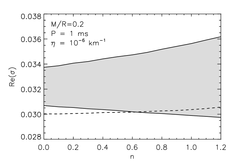
To complete our discussion about the existence of $r$-modes in the continuous spectrum, in Fig. 5 we show the behaviour of the real part of the $r-$mode frequency ($\sigma$) as a function of the polytropic index $n$ for models with compactness $M/R=0.2$, period of 1 ms, and a shear viscosity $\eta=10^{-6}$ km^-1. The period and compactness have been chosen to allow for direct comparison with the results of Ruoff & Kokkotas (2001) who could not find the $r$-modes for $n$ larger than a certain value, when the real part of the frequency reached the continuous spectrum. By introducing a small amount of viscosity, the frequency can be calculated for all polytropic indexes, or for any other stellar model, even if we stay at the most basic level of approximation: first order in the rotation parameter and neglecting the coupling between the axial and polar parts. Note that when the mode lays outside the continuous spectrum we obtain results very similar to Ruoff & Kokkotas (2001).

Some attention must be paid to the fact that viscosity breaks the degeneracy of the $r-$modes and allows for the existence of a family of modes with an arbitrary number of nodes. A simple analytical solution for homogeneous stars in the Newtonian case and for constant $\eta$ is detailed in the Appendix. In this particular case, the eigenfunctions are simply given in terms of the spherical Bessel functions $Z=r~{}j_{l}(kr)$. For the $l=2$ case we have

$$Z\propto\left(3-\frac{1}{(kr)^{2}}\right)\sin{kr}-\frac{3}{kr}\cos{kr}\,.$$ (48)

Indeed, we can obtain a family of solutions labeled by different wave-numbers $k$. In Fig. 6 we show the first three eigenfunctions of the Newtonian $r$ modes for constant density stars and for polytropic stars plotted with dashed and solid lines, respectively. The numerical results for homogeneous stars have been checked to coincide with the above analytical solution. All eigenfunctions have been normalized to their surface value. The analytical solution shows that, for low viscosity, the leading order correction to the frequency is proportional to $\sigma_{0}(\eta/\rho)^{2}-i\eta/\rho$, with $\sigma_{0}=\frac{\Lambda-2}{\Lambda}m\Omega$. The linear dependence of the inverse damping time with $\eta$ has already been discussed in the previous section; here we notice that the correction to the frequency has a quadratic dependence on $\eta$. Remarkably, we find that even for relativistic perturbations, the numerical results can be well fit by this quadratic behaviour with a very good accuracy.

A last relevant result is that in the fully relativistic calculation we could not find more solutions than the fundamental mode. The other overtones found to exist in the Newtonian or Cowling approaches, seem to be incompatible with the pure outgoing wave condition imposed at infinity. In Fig. 7 we show a comparison of relativistic $r-$mode eigenfunctions for constant density stars (for which the inviscid limit is available) with different viscosities: $\eta=0$ (solid), $\eta=1.4\times 10^{-7}$ km^-1 (dots), $\eta=10^{-6}$ km^-1 (dashes), and $\eta=10^{-4}$ km^-1 (dash-dot). The figure shows that the eigenfunction of the fundamental $r-$mode approaches continuously the inviscid limit, which is close to the $r^{3}$ dependence. It should be reminded that both in the Newtonian and in the Cowling approach the gravitational perturbations are neglected; thus, the fact that the relativistic $r-$modes do not admit solutions with large wavenumbers may be an indication that they only exist for fluids where the axial fluid motion is totally decoupled from gravitational perturbations.

4.3 Realistic Neutron Stars

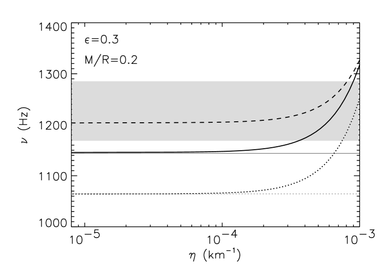
In this section we consider stellar models constructed with realistic EOSs and realistic viscosity profiles with the purpose of establishing if any imprint of the equation of state could be carried by the $r-$mode gravitational wave spectrum. At low density (below $10^{12}$ g/cm³) we use the BPS (Baym et al., 1971) equation of state, while for the inner crust $10^{12}<\rho<10^{14}$ g/cm³ we employ the SLy4 EOS (Chabanat et al., 1998). At high density ($\rho>10^{14}$ g/cm³) we will consider two different EOSs of neutron star matter representative of the two different approaches commonly found in the literature: potential models and relativistic field theoretical models. As a potential model, we have chosen the EOS of Akmal-Pandharipande-Ravenhall (Akmal et al., 1998, hereafter APR). As an example of the mean field solution to a relativistic Walecka–type Lagrangian we have used the parametrization usually known as GM3 (Glendenning & Moszkowski, 1991). For a detailed discussion and comparison of many equations of state from the two families see the recent review by Steiner et al. (2005). Setting the compactness parameter to $M/R=0.2$, APR gives a mass of 1.53 $M_{\odot}$ and a radius of $11.3$ km, while GM3 gives $M=1.72M_{\odot}$ and $R=12.7$ km. For a polytropic EOS with $n=1$ the corresponding mass and radius for the same compactness are $M=1.74~{}M_{\odot}$ and $R=12.8$ km. For cold neutron stars below $10^{9}$ K, neutrons in the inner core become superfluid and the dominant contribution to the shear viscosity is electron-electron scattering (see e.g. the review by Andersson & Kokkotas, 2001); in this regime $\eta$ can be written as

$$\eta_{ee}=6\times 10^{18}\rho_{15}^{2}T_{9}^{-2}~{}{\rm g/cm/s}=1.48\times 10^{-15}\rho_{15}^{2}T_{9}^{-2}~{}{\rm km}^{-1}$$ (49)

with $\rho_{15}$ and $T_{9}$ being the density and temperature in units of $10^{15}$ g/cm³ and $10^{9}$ K. Having this in mind, in this section we will use a viscosity coefficient with a quadratic dependence on density

$$\eta=\eta_{0}\left(\frac{\rho}{\rho_{c}}\right)^{2}~{}{\rm km}^{-1}~{},$$ (50)

where $\rho_{c}$ is the central density. Since old neutrons stars are nearly isothermal, we will parametrize our results as a function of the constant $\eta_{0}$ that includes the temperature dependence.

In Fig. 8 we show the $r-$mode frequency as a function of $\eta_{0}$, comparing the three EOSs: polytrope (dots), APR (dashes) and GM3 (solid lines). In all cases the rotation period is $P=2$ ms. As we can see in the figure, the frequency is rather insensitive to the particular details of the EOS, provided that the rotation frequency and $M/R$ are the same. The Newtonian limit depends only on the angular frequency ($\Omega$) and the relativistic correction enters through the frame dragging. Since this correction goes as $\omega/\Omega\approx I/R^{3}\propto M/R$, the leading order contribution to the frequency is a function only of the compactness.

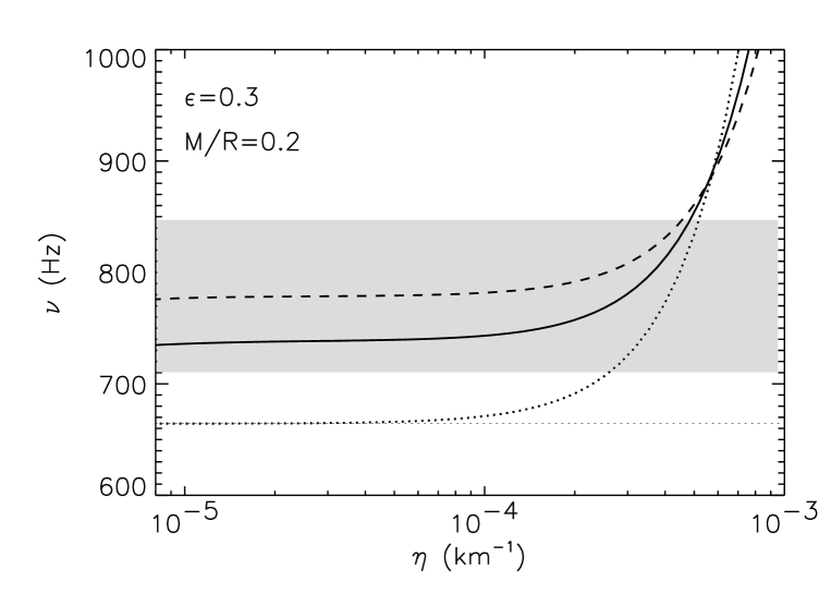
In Fig. 9 we show the damping times for the same models as in Fig. 8. For constant density stars, the $\approx\rho R^{2}$ dependence of the damping time translates into a $M/R$ dependence for models with constant $\eta$. In realistic, cold ($T\lesssim 10^{9}$K) neutron stars, the density is not constant and the viscosity is dominated by the electron-electron scattering process (49). Thus, the analytic result (46) underestimates the viscous damping time. An improved calculation for $n=1$ polytropes taking into account the density profiles and using the shear viscosity (49) (Andersson & Kokkotas 2001) gives

$$\tau=2.2\times 10^{7}\left(\frac{1.4M_{\odot}}{M}\right)\left(\frac{R}{10{\rm km}}\right)^{5}T_{9}^{2}~{}{\rm s}.$$ (51)

Assuming a general dependence of the viscosity of the form of Eq. (50), and using Eq. (49)the above damping time can be shown to satisfy

$$\tau=\left(\frac{1.4M_{\odot}}{M}\right)\left(\frac{R}{10{\rm km}}\right)^{5}\left(\frac{\rho_{c}}{10^{15}{\rm g/cm}^{3}}\right)\left(\frac{3.26\times 10^{-8}{\rm km}^{-1}}{\eta_{0}}\right)~{}{\rm s}.$$ (52)

Our relativistic calculations show approximately the same dependence on mass and radius as Eq. (52), but the damping times are systematically larger of about 60%. We found that a better fit for the realistic neutron stars (APR, GM3) as well as for the $n=1$ polytrope is given by

$$\tau=\left(\frac{1.4M_{\odot}}{M}\right)\left(\frac{R}{10{\rm km}}\right)^{5}\left(\frac{\rho_{c}}{10^{15}{\rm g/cm}^{3}}\right)\left(\frac{5.22\times 10^{-8}{\rm km}^{-1}}{\eta_{0}}\right)~{}{\rm s}.$$ (53)

In Fig. 9 we show, together with the numerical results (thick lines), the results corresponding to the previous fit (thin lines). The good agreement between them is apparent.

5 Final remarks and conclusions

We have investigated the $r-$mode spectrum within a perturbative relativistic framework consistently including the effects of shear viscosity. A first interesting result of our study is that the continuous spectrum, which was an artifact of the level of approximation (first order in rotation, neglecting completely the coupling between polar and axial perturbations), can be regularized and the frequencies and viscous damping times of the modes can be calculated. This can be understood if one analyzes the real cause of the existence of the continuous spectrum. By considering only purely axial perturbations, and working at first order in the rotation parameter, each spherical fluid layer is effectively decoupled from the neighbour (indeed, the perturbations of density, pressure, and radial velocity are zero). Therefore, each layer can oscillate independently and have a different characteristic frequency. This effect can be produced by differential rotation or, in a relativistic framework, by the dragging of the inertial frames. It has been discussed in the literature that including the coupling up to some level, the shape of the continuous spectrum changes (Ruoff & Kokkotas, 2002), but still one cannot always find a mode. In principle, by fully including the coupling (see e.g. Lockitch et al., 2001; Lockitch et al., 2003; Villain & Bonazzola, 2002), one can look for a global mode that oscillates with a unique characteristic frequency, since different layers feel each other and their motion is coupled. We have produced the same effect by introducing shear viscosity. The stress between the different layers couples them and results in the existence of a unique global $r-$mode, instead of a continuous spectrum. Therefore, even working at the most crude level of approximation (purely axial perturbations, first order in rotation) one can calculate the $r-$modes (complex) frequency for every stellar model.

Another interesting outcome of our study is that, in the regime where viscosity dominates, the damping times of relativistic modes are about 40-60% larger than those obtained in the Newtonian case. For homogeneous stars the differences are smaller, and the semi-analytic estimate obtained by Cutler & Lindblom (1987) fits well our numerical results. For realistic neutron stars we find that our relativistic results give damping times systematically larger (about a 60%) than previous Newtonian estimates (Andersson & Kokkotas, 2001), but with the same dependence on mass and radius. An accurate fit to realistic neutron stars, valid also for $n=1$ polytropes gives

$$\tau=3.52\times 10^{7}\left(\frac{1.4M_{\odot}}{M}\right)\left(\frac{R}{10{\rm km}}\right)^{5}T_{9}^{2}~{}{\rm s}~{}.$$ (54)

Notice that the corrections due to general relativity and the internal structure almost cancel each other in such a way that the previous estimate is actually closer to the results for Newtonian constant density stars (Kokkotas & Stergioulas, 1999; Andersson & Kokkotas, 2001) than the more elaborated calculation for $n=1$ polytropes (Andersson & Kokkotas, 2001).

Therefore, we have shown that by including the shear viscosity in the stress-energy tensor we can obtain an accurate estimate of the damping time of the $r-$mode in neutron stars, provided that realistic equation of state and viscosity are known. We were able to extend our results to arbitrarily low viscosity in the Newtonian case, but further improvements, such us including higher order couplings or devising better numerical approaches to deal with smaller values of $\eta$, are needed before we can compute accurately the window of instability of the $r-$modes in a fully relativistic framework. Notice that axial-polar coupling (second order in rotation) must also be included to take into account the effect of bulk viscosity.

In this paper we have not considered the damping associated to the viscous boundary layer in the core-crust interface, which is thought to be one of the most efficient mechanisms to damp the $r-$mode oscillations (Bildsten & Ushomirski 2000; Rieutord 2001). If the crust is assumed to be rigid, the problem can be formulated as an Ekman problem in a spherical layer (Glampedakis & Andersson, 2004). In practice this means to substitute the boundary conditions at the stellar surface by a ”no-slip” condition at the core-crust interface, i.e., $Z(r=R_{c})=0$, and to include the corrections due to the perturbation of the pressure. Shear viscosity in this case is essential since it ensures that the perturbations of the velocity deviate from the inviscid solution and go to zero in a thin layer near the crust (the Ekman layer) with characteristic width $\frac{\Delta r}{R}\approx\sqrt{E_{s}}$. Recent results (Glampedakis & Andersson, 2004) show that the damping rate and the correction to the frequency due to the presence of the Ekman layer go as $(\Omega/R_{c})^{1/2}$, with a numerical factor of the order of unity. This issue will be addressed in a future work.

Acknowledgements

We thank Nils Andersson and Adamantios Stavridis for useful comments and discussions. This work has been supported by the Spanish MEC grant AYA-2004-08067-C03-02, and the Acción Integrada Hispano–Italiana HI2003-0284. J.A.P. is supported by a Ramón y Cajal contract from the Spanish MEC.

Figure 1: The $r-$mode frequency is plotted as a function of the shear viscosity parameter $\eta$ for a uniform density model with $M/R=0.2$ and rotational parameter $\epsilon=0.3$. The Newtonian, Cowling and GR results are shown, respectively, with dotted, dashed, and solid lines. The thin horizontal lines indicate the corresponding Newtonian and GR inviscid limits, while the continuous spectrum is the shadowed region.

Figure 2: The $r-$mode damping time is shown as a function of the shear viscosity parameter $\eta$ for the same model as Fig. 1. The Newtonian, Cowling and GR results are shown, respectively, with dotted, dashed, and solid lines. The thin solid line refers to the simple estimate obtained using Eq. (46).

Figure 3: The $r-$mode frequency is plotted as a function of $\eta$ for a polytropic star with $n=1$, $M/R=0.2$ and rotational parameter $\epsilon=0.3$. The Newtonian, Cowling and GR results are shown, respectively, with dotted, dashed, and solid lines. The horizontal dotted line indicates the corresponding Newtonian inviscid limit, while the continuous spectrum is the shadowed region.

Figure 4: The $r-$mode damping time is plotted as a function of $\eta$ for the same polytropic star of Fig. 3. The Newtonian, Cowling and GR results are shown, respectively, with dotted, dashed, and solid lines. The thin solid line refers to the simple estimate obtained using Eq. (46).

Figure 5: The real part of the $r-$mode frequency is plotted ($\sigma$) as a function of the polytropic index $n$ for models with a shear viscosity parameter $\eta=10^{-6}$ km^-1, compactness $M/R=0.2$ and period of 1 ms.

Figure 6: Newtonian $r-$mode eigenfunctions for constant density stars (dashed lines) and polytropic stars (solid lines) for $\eta=10^{-6}$ km^-1. The numerical results corresponding to constant density stars are found to be in agreement with the analytic eigenfunctions derived in the appendix. The eigenfunctions of polytropic stars have the same qualitative shape.

Figure 7: Comparison of relativistic $r-$mode eigenfunctions for constant density stars and different viscosities: $\eta=0$ (solid), $\eta=1.4\times 10^{-7}$ km^-1 (dots), $\eta=10^{-6}$ km^-1 (dashes), and $\eta=10^{-4}$ km^-1 (dash-dot). In the relativistic case, no mode solution with nodes could be found since only the fundamental $r-$mode admits a pure outgoing wave solution.

Figure 8: Comparison of the $r-$mode frequency as a function of the the viscosity coefficient at the center, $\eta_{0}$, for a polytropic star with $n=1$ (dotted line), the APR (dashed line) and the GM3 (solid line) equations of state. The compactness parameter in all cases is $M/R=0.2$ and the rotation period is 2 ms.

Figure 9: Comparison of the $r-$mode damping time as a function of $\eta_{0}$ for a $n=1$ polytrope (dotted line), the APR (dashed line) and the GM3 (solid line) equations of state, for the same models considered in Fig. 8. The thin lines, whoch show the estimates given by Eq. (53), are difficult to distinguish from the real results.

Appendix A An analytical solution for the Newtonian $r-$modes

The Newtonian equations (29–30) describing the axial perturbations can be written as a single second order ODE

$$r^{2}Z^{\prime\prime}-l(l+1)Z+r^{2}\left(\sigma_{0}\sigma+i\frac{\rho}{\eta}(\sigma-\sigma_{0})\right)Z=0$$ (55)

where $\sigma_{0}$ is the (real) frequency in the inviscid limit $\sigma_{0}=\frac{\Lambda-2}{\Lambda}m\Omega$. If we assume that $\nu\equiv\frac{\eta}{\rho}$ is a constant, this is just a version of the Riccati equation,

$$z^{2}y^{\prime\prime}+\left(k^{2}z^{2}-l(l+1)\right)y=0$$ (56)

which has solutions

$$y=kz(Aj_{l}(kz)+By_{l}(kz))$$ (57)

where $j_{l}(kz)$ and $y_{l}(kz)$ are spherical Bessel functions of the first and second kinds. In our problem we impose regularity of the function at the origin, which implies $B=0$ because $y_{l}(kz)$ diverge in $z=0$. Therefore, we are left with the simple (complex) solution

$$Z=Axj_{l}(x)$$ (58)

where $x=kz$ and $k^{2}=\sigma_{0}\sigma+\frac{i}{\nu}(\sigma-\sigma_{0})$. Notice that this functions have the correct $r^{l+1}$ behaviour near the origin. The eigenmodes and eigenfunctions are then fixed by imposing boundary conditions at a given radius $r=R$. Consider the $l=2$ case and let $A=1$, the solution is:

$$Z(x)=\left(\frac{3}{x^{2}}-1\right)\sin{x}-\frac{3}{x}\cos{x}~{}.$$ (59)

The boundary condition $Z^{\prime}-2Z/r=0$ at $r=R$ implies

$$(5x^{2}-12)\sin{x}-x(x^{2}-12)\cos{x}=0$$ (60)

which has only real solutions. The first few zeros are approximately $x=2.5,7.14,10.5,13.8,17.0~{}~{}...$. The frequency of the fundamental $r-$mode corresponds to $kR=2.5$, but there is an infinite number of higher order overtones. For each wavenumber, the deviation from the inviscid limit ($s\equiv\sigma-\sigma_{0}$) can be readily calculated

$$s=\frac{\left(k^{2}-\sigma_{0}^{2}\right)}{1+\nu^{2}\sigma_{0}^{2}}(\sigma_{0}\nu^{2}-i\nu)~{}.$$ (61)

Notice that in the low viscosity limit, the damping time goes exactly as $\eta/\rho R^{2}$, with a multiplicative factor of order unity, but the correction to the frequency goes as $\eta^{2}$. If the boundary conditions are the no-slip conditions $Z=0$, then we must impose that at $r=R_{c}$

$$\left(3-x^{2}\right)\sin{x}-{3x}\cos{x}=0$$ (62)

whose first zeros are $x=5.75,9.1,12.3,15.5~{}...$

We have checked that the numerical results show the same qualitative dependence, even for polytropic or realistic stars. Knowing the dependence in the low viscosity limit allows us to regularize the equations and solve them numerically with arbitrarily small viscosity. Using $\bar{s}=s/\eta$ as a variable, the Newtonian equations (29–30) become

$$Z^{\prime} = \frac{2}{r}Z+X$$ (63)

$$X^{\prime} = -\frac{2}{r}X+\frac{(\Lambda-2)}{r^{2}}Z-(\sigma_{0}(\sigma_{0}+\eta\bar{s})+{\rm i}{\rho}\bar{s})Z$$ (64)

and can be integrated numerically since $\bar{s}$ is well behaved as $\eta\rightarrow 0$.

A last important remark is that for low viscosity all the overtones have very close frequencies ($\eta^{2}$ corrections), but the damping times scale with $k^{2}-\sigma_{0}^{2}\approx k^{2}$, so that modes with shorter wavelength are damped faster than the fundamental mode (typically a factor 4-10). Therefore, understanding the non-linear transfer of energy between the fundamental $r-$mode and higher order overtones may be relevant for astrophysical applications.

References

- [1] Akmal A., Pandharipande V.R., Ravenhall D.G., 1998, Phys.Rev. C, 58, 1804
- [2] Andersson N., 1998, ApJ, 502, 708
- [3] Andersson N., Comer G.L, Glampedakis K., 2004, astro-ph/0411748
- [4] Andersson N., 2003, Class.Quant.Grav., 20, R105
- [5] Andersson N., Jones D.I., Kokkotas K.D, 2002, MNRAS, 337, 1224
- [6] Andersson N., Kokkotas K.D., 2001, Int.Jour.Mod.Phys. D, 10, 381
- [7] Andersson N, Kokkotas K.D., Schutz B.F., 1995, MNRAS, 274, 1039
- [8] Andersson N, Kokkotas K.D., Schutz B, 1999, ApJ, 510, 846
- [9] Baym G., Pethick C.J., Sutherland P., 1971, ApJ, 170, 299
- [10] Bildsten L, 1998, ApJL, 501, L89
- [11] Bildsten L., Ushomirsky G., 2000, ApJL, 529, L33
- [12] Chabanat E., et al., 1998, Nucl. Phys, A., 635, 231
- [13] Cutler C., Lindblom L., 1987, ApJ, 314, 234
- [14] Glampedakis K., Andersson N., 2004, astro-ph/0411750
- [15] Glendenning, N.K., Moszkowski, S., 1991, Phys. Rev. Lett., 67, 2414
- [16] Gressman P., Lin L-M, Suen W-M, Stergioulas N., Friedman J.L., 2002, Phys. Rev. Rapid Comm., D66 041303(R)
- [17] Gualtieri L., Pons J.A., Miniutti G., 2004, Phys.Rev. D, 70, 084009
- [18] Hartle J.B., 1967, ApJ, 150, 1005
- [19] Hartle J.B., Thorne K.S., 1968, ApJ, 153, 807
- [20] Israel W., 1966, Nuovo Cimento, 44, 1
- [21] Kojima Y., 1992, Phys. Rev D, 46, 4289
- [22] Kojima Y., 1993, ApJ, 414, 247
- [23] Kojima Y., 1998, MNRAS, 293, 49
- [24] Kokkotas K.D., Schmidt B.G., 1999, Living Rev. Relativity, 2, http://www.livingreviews.org/lrr-1999-2
- [25] Kokkotas K.D., Stergioulas N., 1999, A&A, 341, 110
- [26] Leaver E.W., 1985, Proc. R. Soc. London, A402, 285
- [27] Leins M., Nollert H.P., Soffel M.H., 1993, Phys.Rev. D, 48, 3467
- [28] Lindblom L., Owen B.J., Morsink S.M., 1998, Phys. Rev. Lett., 80, 4843
- [29] Lindblom L., Owen B.J., 2002, Phys.Rev. D, 65, 063006
- [30] Lockitch K.H., Andersson N., Friedman J.L., 2001, Phys.Rev. D, 63, 024019
- [31] Lockitch K.H., Andersson N., Friedman J.L., 2003, Phys.Rev. D, 68, 124010
- [32] Lockitch K.H., Andersson N., Watts A.L., 2004, Class.Quant.Grav., 21, 4661
- [33] Misner C.W., Thorne K.S., Wheeler J.A., 1973, in Gravitation, W H Freeman & C, New York
- [34] Price R., Thorne K.S., 1969, ApJ, 155, 163
- [35] Rieutord M., 2001, ApJ, 550, 443
- [36] Ruoff J., Kokkotas K.D., 2001, MNRAS, 328, 678
- [37] Ruoff J., Kokkotas K.D., 2002, MNRAS, 330, 1027
- [38] Ruoff J., Stavridis A., Kokkotas K.D., 2002, MNRAS, 332, 676
- [39] Steiner A.W., Prakash M., Lattimer J.M., Ellis P.J., 2005, Physics Reports in press, nucl-th/0410066
- [40] Thorne K.S., Campolattaro A., 1967, ApJ, 149, 591
- [41] Villain L., Bonazzola S., 2002, Phys.Rev. D, 66, 123001
- [42] Wagoner R., 2002, ApJ, 578, L63