Multicolour photometry of Balloon 090100001: linking the two classes of pulsating hot subdwarfs

Abstract

We present results of the multicolour $UBVR$ photometry of the high-amplitude EC 14026-type star, Balloon 090100001. The data span over a month and consist of more than a hundred hours of observations. Fourier analysis of these data led us to the detection of at least 30 modes of pulsation of which 22 are independent. The frequencies of 13 detected modes group in three narrow ranges, around 2.8, 3.8 and 4.7 mHz, where the radial fundamental mode, the first and second overtones are likely to occur. Surprisingly, we also detect 9 independent modes in the low-frequency domain, between 0.15 and 0.4 mHz. These modes are typical for pulsations found in PG 1716+426-type stars, discovered recently among cool B-type subdwarfs. The modes found in these stars are attributed to the high-order $g$ modes. As both kinds of pulsations are observed in Balloon 090100001, it represents a link between the two classes of pulsating hot subdwarfs. At present, it is probably the most suitable target for testing evolutionary scenarios and internal constitution models of these stars by means of asteroseismology.

Three of the modes we discovered form an equidistant frequency triplet which can be explained by invoking rotational splitting of an $\ell$ = 1 mode. The splitting amounts to about 1.58 $\mu$Hz, leading to a rotation period of 7.1 $\pm$ 0.1 days.

1 Introduction

Soon after the discovery of about a dozen pulsating B-type subdwarfs (sdB) by the South African Astronomical Observatory astronomers [Kilkenny et al. (1997) and the next papers of the series], two other groups (Billéres et al. 2002, Østensen et al. 2001a,b, Silvotti et al. 2002a) undertook extensive searches for these interesting multiperiodic pulsators, called—after the prototype—the EC 14026 stars. The searches resulted in finding further variables, so that there are 32 EC 14026 stars known at present. Their pulsation periods range between 1.5 and 10 minutes, with a typical value of 2–3 minutes. The amplitudes are rather small and rarely exceed 10 mmag. Some extreme cases are known, however. The longest periods are observed among the members having the lowest surface gravity: V 338 Ser = PG 1605+072 (Koen et al. 1998a, Kilkenny et al. 1999), KL UMa = Feige 48 (Koen et al. 1998b, Reed et al. 2004a), HK Cnc = PG 0856+121 (Piccioni et al. 2000, Ulla et al. 2001), V 2214 Cyg = KPD 1930+2752 (Billéres et al. 2000), V 391 Peg = HS 2201+2610 (Østensen et al. 2001a, Silvotti et al. 2002b), and HS 0702+6043 (Dreizler et al. 2002). Some of them (e.g., V 338 Ser and HS 0702+6043) have large amplitudes. Recently, Oreiro et al. (2004) discovered another high-amplitude and cool EC14026 star, Balloon 090100001 = GSC 02248-01751 (hereafter Bal09). The semi-amplitude of one of the detected modes amounts to 60 mmag in white light, the largest amplitude known in an EC14026 star. With $B\approx$ 11.8 mag, the star is actually one of the brightest members of the group.

B-type subdwarfs are believed to be low-mass ($\sim$0.5 $M_{\odot}$) evolved stars that burn helium in their cores (Heber 1986, Saffer et al. 1994). In the H-R diagram they populate the extended horizontal branch (EHB) region. As their hydrogen envelopes are very thin, they do not ascend the asymptotic giant branch and do not pass the planetary nebula phase of evolution (Greggio & Renzini, 1990). Instead, they evolve almost directly to the white-dwarf stage, passing only through the hotter sdO phase (Dorman et al., 1995). Their evolutionary past, however, is not well understood. The discovery of pulsations in sdB stars opened therefore a new way for investigating their internal structure by means of asteroseismology (see, e.g., Brassard et al. 2001). The effective temperatures of EC14026 stars range from 29 000 to 36 000 K, their surface gravities, $\log g$ = 5.2–6.1. They do not occupy, however, a well-defined instability strip in the $\log T_{\rm eff}$–$\log g$ plane but are spread among non-pulsating sdB stars. Curiously enough, their pulsations were predicted almost at the time of discovery (Charpinet et al., 1996) as corresponding to radial and nonradial low-order low-degree $p$ modes driven by the $\kappa$ mechanism. The driving comes from the metal opacity bump that originates from the ionization of heavy metals, mainly iron (Charpinet et al. 1997, 2001).

About two years ago, Green et al. (2003) discovered low-amplitude multiperiodic light variations with periods of the order of one hour among the coolest ($T_{\rm eff}<$ 30 000 K) sdB stars. The periods of the members of this new class of variable stars indicate that they are high-order $g$ modes. Although Green et al. (2003) announced the discovery of 20 stars of this type, detailed analysis was so far published only for the prototype, PG 1716+426 (Reed et al., 2004a). The pulsations were explained by means of the same pulsation mechanism as the short-period ones (Fontaine et al., 2003), but with degrees $\ell$ = 3 or 4. As far as the effective temperature and the character of excited modes are concerned, the two classes of variable sdB stars resemble younger main-sequence pulsators, $\beta$ Cephei and SPB stars (see, e.g., Pamyatnykh 1999). In the $\log T_{\rm eff}$–$\log g$ plane, the areas where the EC14026 stars and their long-period counterparts are found slightly overlap. It seems therefore possible that both kinds of pulsations observed in sdB stars might coexist in a single star of this type.

The sdB nature of Bal09 was discovered by Bixler et al. (1991) using the balloon-borne SCAP ultraviolet telescope. Its short-period variability was detected by Oreiro et al. (2004) by means of the 80-cm IAC80 telescope at Observatorio del Teide (Tenerife). The effective temperature of 29 500 K and $\log g\approx$ 5.3, derived by the same authors, place it among the coolest and most evolved EC14026 stars. From the data obtained on a single observational night, Oreiro et al. (2004) were able to detect only two independent modes. Owing to the large amplitude and relatively long periods, the star was an obvious target for follow-up time-series photometry. We therefore decided to carry out multicolour observations of this star. New observations were also obtained by the discoverers (Oreiro, private communication). In this paper, we present the results of our photometric run, covering over a month. We show that Bal09 exhibits both kinds of pulsations discovered in sdB stars.

2 Observations and reductions

We started observing Bal09 on June 30, 2004. The bulk of the data was, however, obtained between August 17 and September 19, 2004, on 18 nights. All these observations were obtained at Mt. Suhora Observatory with a 60-cm reflecting telescope, equipped with the ST-10XME CCD camera and Johnson-Cousins $UBVR$ filters. The camera field of view was 6.8 $\times$ 4.5 arcmin and, in order to minimize storage time, the 3 $\times$ 3 pixels on-chip binning was employed. Except for the first night, June 30, when only $R$ filter was used, and the second night, when $V$-filter measurements were not made, the observations were carried out through four filters, $U$, $B$, $V$, and $R$. The mean exposure times amounted respectively to 15, 10, 7 and 7 s, resulting in about 1 minute-long filter cycle. This enabled us to obtain roughly 6 points per main pulsation period of Bal09 in all four filters. In total, 125 hours of observations were obtained in the $U$ and $B$ filters, 119 in $V$, and 126 in $R$.

Additional observations were carried out on three observing nights between September 22 and 25, 2004, at Loiano Observatory with the 1.52-m Cassini telescope and the BFOSC CCD camera covering 13 $\times$ 12.6 arcmin on the sky. In total, we gathered 13 hours of observations only in filter $V$. The exposure times were 10 or 15 s long, depending on sky conditions. The time distribution of all observations is shown in Fig. 1.

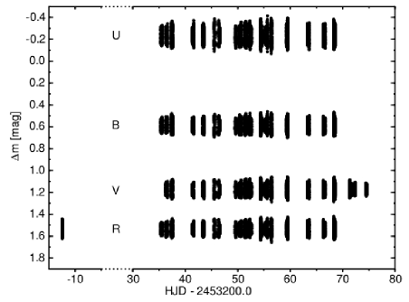
Figure 1: Differential $UBVR$ magnitudes of Bal09 obtained during our run, plotted against heliocentric Julian Day. The observations were obtained at Mt. Suhora Observatory, except those on the last three nights in $V$ that were taken at Loiano Observatory.

Over 7000 individual frames were obtained in $U$, $B$ and $R$ and about 8500 in $V$. All these frames were corrected for bias, dark and flatfield in a standard way. Then, the magnitudes of all stars detected in a frame were obtained by means of profile-fitting procedures of the Daophot package (Stetson, 1987). The aperture magnitudes were also derived. In order to minimize photometric errors, the apertures were scaled with seeing. As a measure of seeing, we used the $\sigma$s of the two-dimensional Gaussian function that described the analytical part of the point-spread function (PSF) calculated by Daophot. The positions of the stars were also taken from the PSF fits. The seeing scaling factor, optimal from the point of view of the photometric errors, depended on the aperture magnitude of a star. We derived the character of this dependence from the post-fit residuals on a single good night and then applied it to all observations. As a comparison star, we chose the nearby, relatively bright star, GSC 02248-00063. It is brighter than Bal09 in $B$, $V$, and $R$, but slightly fainter in $U$. As can be seen in Fig. 1, the mean differential magnitudes range from $-$0.23 mag in $U$ to 1.54 mag in $R$. This large range reflects large differences in colour between Bal09 and the comparison star. Surprisingly, there is practically no difference between the mean differential magnitudes for the $V$-filter data from Mt. Suhora and Loiano. This means that the instrumental systems in both sites are very similar and the $V$ data can be safely combined.

The differential aperture photometry showed less scatter than the PSF photometry. Consequently, for the frequency analysis that follows, we used the aperture photometry. One night’s sample differential magnitudes in $V$ are shown in Fig. 2.

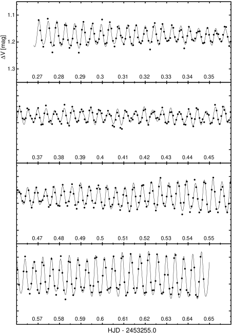
Figure 2: Observations of Bal09 on a single night (September 6, 2004) obtained at Mt. Suhora Observatory in filter $V$. The solid line is the synthetic light-curve consisting of 30 periodic terms listed in Table 1.

3 Frequency analysis

Prior to the frequency analysis, we rejected data points that had photometric errors larger than a certain, arbitrarily chosen value, viz., 0.04 mag for $U$, 0.03 mag for $B$, and 0.025 mag for $V$ and $R$. As the amplitudes of the light variation of Bal09 are quite large, the next three steps, i.e., rejecting outliers, correcting for second-order extinction effects and detrending, were done using the residuals from a preliminary fit. For this purpose, sequential prewhitening was done, until all periodic terms with signal-to-noise (S/N) ratio larger than 6 were subtracted from the data.

Having obtained the residuals, we first rejected all outliers from the original data employing 5-$\sigma$ clipping. Since the comparison star is much redder than Bal09, and we made observations through wide-band filters, second-order extinction effects can be expected. In order to correct for them, we plotted the residuals, $\Delta m_{\rm res}$, obtained earlier, against the air mass, $X$, and derived the coefficients of the relation

$$\Delta m_{\rm res}=a(X-\mbox{1.25})+b$$

by means of the least-squares method. The linear coefficient, $a$, was significantly different from zero and amounted to +0.044, +0.033, +0.009, and +0.012 $\pm$ 0.001 for $U$, $B$, $V$, and $R$, respectively. The $a(X-\mbox{1.25})$ factor was then subtracted from the original data. Finally, the prewhitening was repeated and new residuals were computed.

Because 90% of our data in $V$ and all data in the remaining three filters come from the same telescope/detector combination, they constitute a very homogeneous dataset. Nevertheless, some instrumental effects can produce artificial trends in the data, increasing amplitudes at the lowest frequencies, making it difficult to say which low-frequency signals are real. We will discuss this problem in Sect. 3.7 using data that were not detrended. At the present stage, detrending was performed, again using the residuals. First, the average magnitudes in 0.07-day intervals were calculated and then interpolated using the cubic spline fit. This fit was subtracted from the original data. The 0.07-day interval was chosen by trial and error. This choice secures that all signals at frequencies below $\sim$0.1 mHz are effectively reduced while those with higher frequencies, where $g$ modes are observed (Sect. 3.2), remain unaffected.

3.1 Detected frequencies

Detrended data were analyzed by means of the standard procedure that included calculating the Fourier amplitude periodograms and sequential prewhitening of detected signals. At each step of prewhitening, the parameters of sinusoidal terms found earlier were improved by means of the non-linear least-squares method. Data in each filter were analyzed independently. The periodogram of the $V$-filter data, up to the frequency of 10 mHz, is shown in Fig. 3. The structure of the aliases can be seen in Fig. 4, where we show Fourier periodogram of artificial data containing a single sinusoidal term with frequency and amplitude of the main mode and distributed in time as the real observations in $V$. The daily aliases are quite high, as both sites where the $V$ observations were carried out are located at a similar longitude. Therefore, the frequencies we derive, especially the low-amplitude ones, may suffer from the 1 (sidereal day)^-1 = 11.6 $\mu$Hz ambiguity. Our data cover 35 days, resulting in a frequency resolution of about 0.5 $\mu$Hz (Loumos & Deeming, 1978).

Figure 3: Fourier amplitude periodogram of the detrended $V$-filter data of Bal09. The highest peak at about 2.8 mHz is truncated; its height is equal to about 53 mmag.

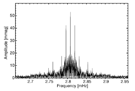
Figure 4: Fourier amplitude periodogram of the artificial data containing a single sinusoidal term with frequency of 2.8074594 mHz and amplitude of 53.3 mmag, distributed in time as the real observations in $V$.

The Fourier spectrum of Bal09 shown in Fig. 3 is dominated by the strong peak around $f\approx$ 2.8 mHz and its daily aliases. It is the main frequency discovered by Oreiro et al. (2004). Signals at the harmonics, 2$f$ (5.6 mHz) and 3$f$ (8.4 mHz), can also be seen. The second frequency detected by these authors, at about 3.8 mHz, is also well seen. In addition, we see low-amplitude peaks at 4.7 mHz and, surprisingly, at low frequencies below 0.4 mHz. Note that the peak at frequency of 0.3 mHz was already detected by Oreiro et al. (2004), but these authors were not able to attribute it convincingly to the star because of the very short time interval of their observations.

The analysis was carried out until all terms with S/N $>$ 4.5 were extracted. The number of periodic terms found in this way was not the same in all filters, mainly due to the differences in the detection threshold. The threshold was the lowest in $V$, where we found 27 independent terms and 7 combinations terms, including harmonics. In $U$, we found 20 + 3, in $B$, 22 + 3, and in $R$, 23 + 6 terms. Of all these terms, 17 (including 3 combination terms) were found in all four filters. We finally adopted a model consisting of 22 independent terms and 8 combination terms. The model comprised all terms detected in $V$ and at least one other filter, and all combination terms. The frequencies of all terms included in this model and the results of the fit of this model to our multicolour time-series data are presented in Table 1.

Table 1: Frequencies, $UBVR$ semi-amplitudes, and phases of 30 sinusoidal terms adopted in the pulsation model of Bal09. Terms in a given frequency range are listed according to decreasing $V$ amplitude. Amplitudes in square brackets indicate that the term was not detected in the data obtained in a given filter. Phases are given for the epoch HJD 2453252.0, the errors of their last digits are given in parentheses. The entries at the bottom of the table give global parameters of the fit. $N_{\rm obs}$ denotes the number of the data points in a given filter, $\sigma_{\rm A}$, the rms error of the semi-amplitude, and $\Delta m$, the mean differential magnitude (variable $-$ comparison). Detection threshold corresponds to S/N = 4.5 in the Fourier periodogram of the residuals.

Frequency		Period	Semi-amplitude [mmag]				Phase [rad]
[mHz]		[s]	$A_{\rm U}$	$A_{\rm B}$	$A_{\rm V}$	$A_{\rm R}$	$\phi_{\rm U}$	$\phi_{\rm B}$	$\phi_{\rm V}$	$\phi_{\rm R}$
$f_{\rm A}$	0.272385 $\pm$ 0.000014	3671.27	3.11	2.55	2.19	2.23	3.89(08)	3.85(07)	3.86(07)	3.78(07)
$f_{\rm B}$	0.365808 $\pm$ 0.000012	2733.67	3.29	2.81	2.13	2.30	2.80(08)	2.87(06)	2.74(07)	2.76(07)
$f_{\rm C}$	0.325644 $\pm$ 0.000019	3070.84	2.18	1.54	1.92	1.53	3.64(11)	3.52(11)	3.65(08)	3.45(11)
$f_{\rm D}$	0.239959 $\pm$ 0.000020	4167.38	2.24	2.00	1.59	1.87	4.84(12)	4.85(09)	4.79(10)	5.01(09)
$f_{\rm E}$	0.15997 $\pm$ 0.00003	6251.2	1.18	[0.80]	1.22	[0.68]	5.20(21)	5.44(22)	5.02(12)	5.15(24)
$f_{\rm F}$	0.24629 $\pm$ 0.00004	4060.3	[1.08]	[0.67]	1.14	0.86	4.79(25)	4.44(28)	4.80(14)	4.15(20)
$f_{\rm G}$	0.29897 $\pm$ 0.00004	3344.8	[1.14]	1.02	1.08	[0.70]	2.58(22)	2.66(17)	2.50(14)	2.70(24)
$f_{\rm H}$	0.20194 $\pm$ 0.00003	4952.7	1.42	0.98	1.04	[0.48]	0.26(18)	0.54(18)	0.22(15)	0.50(35)
$f_{\rm I}$	0.22965 $\pm$ 0.00003	4354.5	1.54	0.96	0.84	0.84	2.89(17)	2.74(19)	2.73(19)	3.13(20)
$f_{1}$	2.8074594 $\pm$ 0.0000006	356.19393	75.23	57.71	53.34	50.26	2.099(04)	2.112(03)	2.112(03)	2.108(03)
$f_{2}$	2.8232252 $\pm$ 0.0000017	354.20483	26.71	21.92	20.53	19.92	1.137(10)	1.149(09)	1.143(08)	1.123(09)
$f_{3}$	2.824799 $\pm$ 0.000003	354.0075	15.82	12.86	11.62	11.57	5.359(16)	5.347(14)	5.328(14)	5.344(15)
$f_{4}$	2.826384 $\pm$ 0.000007	353.8090	5.86	5.12	4.71	4.59	0.95(04)	0.90(04)	0.77(03)	0.88(04)
$f_{5}$	2.85395 $\pm$ 0.00003	350.392	2.23	1.81	2.08	1.45	5.15(12)	4.95(10)	4.95(08)	5.15(12)
$f_{6}$	2.85852 $\pm$ 0.00003	349.831	1.94	1.45	1.58	1.45	0.68(14)	0.86(13)	0.81(10)	0.86(12)
$f_{7}$	2.85567 $\pm$ 0.00003	350.181	2.01	1.72	1.31	1.48	1.87(13)	1.76(11)	1.99(12)	1.85(11)
$f_{8}$	3.776084 $\pm$ 0.000008	264.8246	5.94	4.73	4.16	4.07	1.16(04)	1.15(04)	1.16(04)	1.13(04)
$f_{9}$	3.786788 $\pm$ 0.000017	264.0760	2.58	1.83	1.51	1.60	6.04(10)	5.96(10)	5.80(10)	5.92(11)
$f_{10}$	3.79556 $\pm$ 0.00003	263.466	[1.37]	1.14	1.46	1.20	2.16(18)	2.34(16)	1.51(10)	2.12(14)
$f_{11}$	4.64508 $\pm$ 0.00003	215.282	[1.07]	0.96	1.15	0.90	2.15(24)	2.19(19)	2.16(13)	2.42(19)
$f_{12}$	4.66953 $\pm$ 0.00003	214.154	[0.82]	1.07	0.88	[0.69]	1.82(30)	1.72(17)	1.98(17)	1.77(24)
$f_{13}$	4.66135 $\pm$ 0.00004	214.530	1.35	[1.00]	0.70	[0.74]	2.29(19)	2.09(18)	2.46(21)	2.72(23)
2$f_{1}$	5.6149188 $\pm$ 0.0000012	178.09697	7.36	6.04	5.77	5.27	5.78(04)	5.84(03)	5.93(03)	5.88(03)
$f_{1}+f_{2}$	5.6306846 $\pm$ 0.0000018	177.59830	5.48	4.35	4.10	3.96	4.94(05)	4.91(04)	4.95(04)	4.92(04)
$f_{1}+f_{3}$	5.632259 $\pm$ 0.000004	177.5487	3.05	2.51	2.61	2.50	3.01(09)	2.96(07)	2.88(07)	2.96(07)
$f_{1}+f_{4}$	5.633843 $\pm$ 0.000007	177.4987	[1.01]	[1.08]	1.03	0.92	4.44(27)	4.88(18)	4.72(16)	4.53(20)
3$f_{1}$	8.4223782 $\pm$ 0.0000018	118.73131	[0.85]	[0.68]	0.95	0.96	3.53(30)	3.59(26)	3.87(16)	3.66(17)
$f_{1}-f_{\rm B}$	2.441651 $\pm$ 0.000012	409.5589	[1.06]	[0.75]	0.82	[0.73]	2.79(23)	2.79(24)	2.55(18)	2.99(22)
$f_{2}+f_{3}$	5.648024 $\pm$ 0.000005	177.0531	[0.91]	[0.73]	0.81	[0.55]	2.37(29)	1.93(26)	2.43(20)	2.19(32)
2$f_{1}+f_{2}$	8.438144 $\pm$ 0.000003	118.5095	[0.69]	[0.42]	[0.58]	0.94	2.58(37)	2.10(43)	3.11(27)	2.48(18)
$\sigma_{\rm A}$ [mmag]			0.25	0.18	0.16	0.17
Nobs			7154	7197	8529	7382
Residual SD [mmag]			14.80	10.54	9.59	9.96
Detection threshold [mmag]			1.38	0.97	0.82	0.88
$\Delta m$ [mag]			$-$0.2290	0.5940	1.1771	1.5389

It is clearly seen from Table 1 (see also Fig. 1) that the frequencies of modes detected in Bal09 cluster in four narrow frequency ranges: below 0.4 mHz, around 2.8, 3.8, and 4.7 mHz. After removing the 30 terms from the data, the Fourier spectra of the residuals still exhibit an excess power in these four ranges (Fig. 5). Because the noise level increases towards low frequencies, we stopped extracting terms with frequencies below 1 mHz. However, extracting all terms down to S/N = 4.5 for frequencies in the range 1–10 mHz, led us to detecting additional 9 low-amplitude terms. Their frequencies are listed in Table 2. Note that only some are found in two bands, and even in these cases there is an ambiguity in frequency because of aliasing. It is clear that multi-site data are necessary to verify the reality of these terms.

Figure 5: Fourier spectra of the $UBVR$ residuals after removing 30 terms listed in Table 1.

Table 2: Additional high-frequency terms with S/N $>$ 4.5 found in the residuals.

	Detected frequency [mHz]
$f_{i}$	$U$	$B$	$V$	$R$	Comment
$f_{14}$	—	—	2.80599	—
$f_{15}$	—	—	—	3.76367
$f_{16}$	—	—	—	3.79036
$f_{17}$	—	3.80592	—	3.79430	daily aliases
$f_{18}$	3.80921	3.79767	—	—	daily aliases
$f_{19}$	—	—	3.80509	—
$f_{20}$	—	—	3.80670	—
$f_{21}$	—	4.64441	—	—
$f_{22}$	—	—	4.67491	—

We will now discuss frequency contents of the multicolour data of Bal09 in the four frequency ranges mentioned above, illustrating the discussion with the Fourier amplitude spectra in the $V$ filter obtained at different steps of prewhitening.

3.2 Low-frequency region (0.15–0.4 mHz)

Out of 22 independent terms included in the model listed in Table 1, nine were found in the low-frequency range, between 0.15 and 0.4 mHz. Five ($f_{\rm A}$ to $f_{\rm D}$ and $f_{\rm I}$) were detected in all four filters. The Fourier spectrum in this range (Fig. 6) shows complicated structure; the first four terms have amplitudes of about 2 mmag in $V$, the remaining ones are even weaker. The dense spectrum of terms with low amplitudes in this range causes that aliasing is really a problem here.

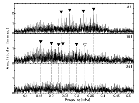
Figure 6: Fourier amplitude spectra of the $V$ data of Bal09 in the low-frequency domain. The number on the right shows how many periodic terms were extracted from the data before calculating the periodogram. Vertical dashed lines correspond to frequencies that have been already extracted. The inverted filled triangles indicate frequencies included in the model given in Table 1, the open triangle, that detected only in $V$ data.

3.3 The 2.8 mHz region

The strong peak at frequency of about 2.81 mHz, found by Oreiro et al. (2004), is resolved in our data into several components. The strongest component has frequency $f_{1}$ = 2.8074594 $\pm$ 0.0000006 mHz (period 356.2 s) and is non-sinusoidal in shape, as we detected two its harmonics. All combination frequencies we detected, except $f_{2}+f_{3}$, involve $f_{1}$. The 6-minute oscillations corresponding to $f_{1}$ dominate the light curve of Bal09 (see Fig. 2). We detected six terms in the vicinity of $f_{1}$ that were included in the 30-term model. One of the most interesting features seen in Fig. 7 is that $f_{2}$, $f_{3}$, and $f_{4}$ form an equidistant frequency triplet.

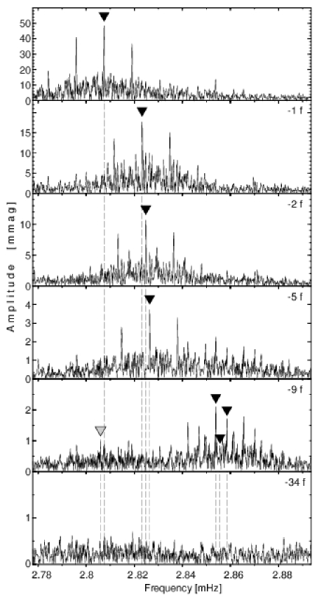
Figure 7: Fourier amplitude spectra of the $V$ data of Bal09 in the vicinity of the main mode, $f_{1}$ = 2.80746 mHz. Notation is the same as in Fig. 6, except that the frequency listed in Table 2 is indicated by the inverted gray triangle. Note the differences in the ordinate scale.

The frequency differences between the components of the triplet are the same within the errors and amount to: $f_{3}-f_{2}$ = 1.574 $\pm$ 0.003 $\mu$Hz and $f_{4}-f_{3}$ = 1.585 $\pm$ 0.008 $\mu$Hz. Thus, they can be resolved only if observations cover more than a week. It is natural to suggest that the triplet is a rotationally split one; we will return to this interpretation in Sect. 5.3. The beat period between $f_{1}$ and the triplet components is of the order of 0.7 d, and this beating is responsible for the changes of amplitude in the observed light curve (Fig. 2).

At a frequency about 0.03 mHz larger than that of the triplet, three next frequencies were resolved. They are closely, although not equally spaced, $f_{7}-f_{5}$ = 1.72 $\pm$ 0.04 $\mu$Hz, $f_{6}-f_{7}$ = 2.85 $\pm$ 0.04 $\mu$Hz.

One additional term was found in the 2.8 mHz region in the residuals of the 30-term model (Table 2). This $f_{14}$ term, found only in the $V$ data (Fig. 7), lies very close to the combination frequency $f_{1}+f_{2}-f_{3}\approx f_{1}+f_{3}-f_{4}$, but if real, it is more likely to be an independent mode. The reason is that a much higher amplitude is found when solving for this frequency rather than assuming that it has a combination value. The difference $f_{1}-f_{14}$ is equal to 1.46 $\pm$ 0.03 $\mu$Hz.

3.4 The 3.8 mHz region

A peak at 3.78 mHz was already seen by Oreiro et al. (2004) in their Bal09 observations. We resolve it into three terms, counting only those that appear in Table 1 or nine, if those from Table 2 are taken into account. It is interesting to note that $f_{20}-f_{19}$ = 1.61 $\pm$ 0.04 $\mu$Hz, a value that, to within the errors, is the same as the separation of the three frequencies around 2.825 mHz. As can be seen from Fig. 8 (but see also Fig. 5), the region is rich in low-amplitude modes. Not all can be identified unambiguously from our data due to aliasing and the fact that many appear only in one periodogram.

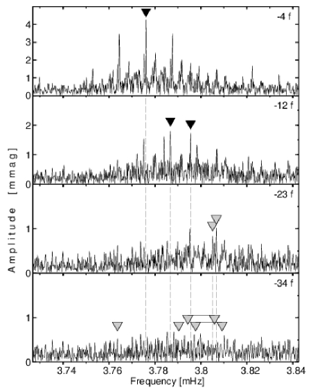
Figure 8: Fourier amplitude spectra of the $V$ data of Bal09 around frequency 3.8 mHz, showing representative steps of prewhitening. Symbols are the same as in Figs. 6 and 7. Note that out of six additional frequencies (Table 2), indicated by the gray triangles, two were found in the $V$ data only. These two are shown in the second panel from the bottom, the remaining four, in the bottom panel. Triangles indicating alias frequencies are connected with horizontal lines.

3.5 The 4.7 mHz region

Modes with frequencies around 4.7 mHz were not detected by Oreiro et al. (2004). We included three terms from this region in our 30-term model, but two more are detected with S/N $>$ 4.5: one in $B$ and one in $V$ (Fig. 9). All terms in this region have very small amplitudes, around 1 mmag or even smaller.

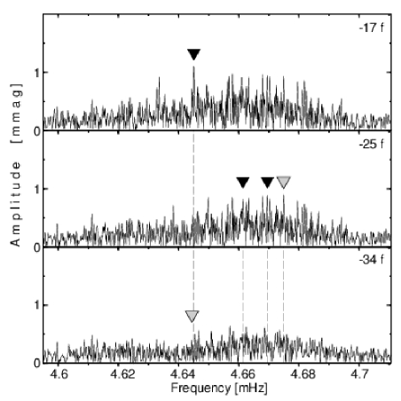
Figure 9: The same as Fig. 8, but around frequency 4.7 mHz.

3.6 Combination frequencies

The combination frequencies appear in three distinct regions (see Fig. 10 and Table 1). The richest is the 5.6 mHz region where the 2$f_{1}$ harmonic and the sums of the highest-amplitude terms occur. Five combination frequencies are detected in this region, including the sum of $f_{1}$ and all three triplet components, as well as $f_{2}+f_{3}$.

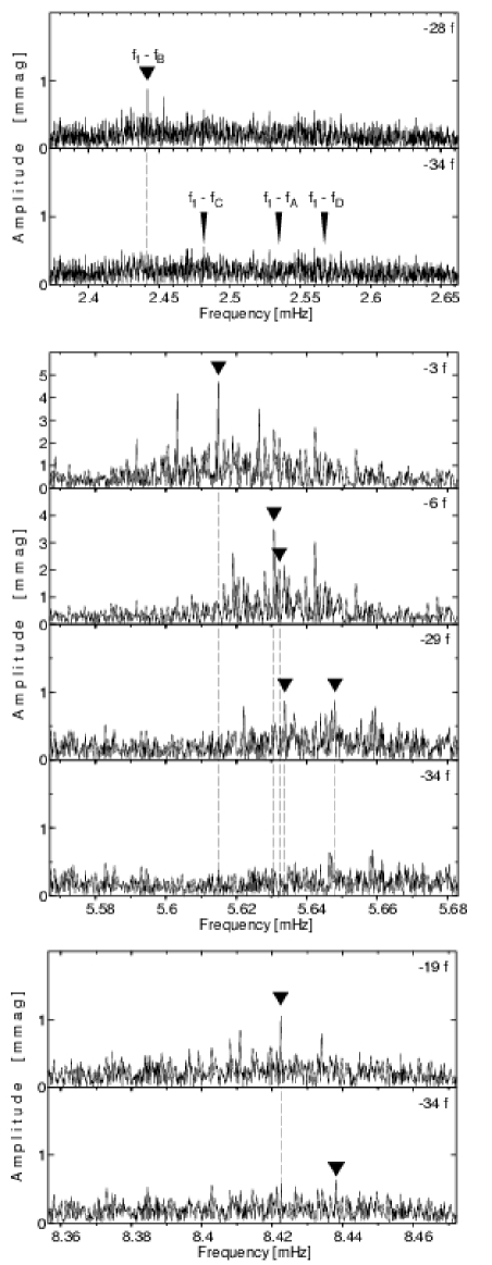
Figure 10: The same as Fig. 8, but in three regions where the combination frequencies occur. See text for the explanation of the difference terms indicated in the top panel.

In the 8.4 mHz region, the 3$f_{1}$ term is detected only in $V$. However, although not detected above S/N = 4.5, the 2$f_{1}$ + $f_{2}$ is also very well seen in the periodogram of the residuals (Fig. 10).

For the assessment of reality of the signals, the most important is, however, the detection of the difference term $f_{1}-f_{\rm B}$ at 2.441651 mHz (see Fig. 10, top panel). This combination term involves frequencies from the high and low-frequency ranges. Its occurence proves that both $f_{1}$ and $f_{\rm B}$ originate in the same star. In Fig. 10 we have also indicated the difference combination terms between $f_{1}$ and three other low-frequency terms with the largest amplitudes. A detailed look at the residual spectrum in $V$ shows that in addition to the peak at $f_{1}-f_{\rm B}$ there is also a low but still noticeable peak at $f_{1}-f_{\rm C}$ = 2.48165 mHz.

3.7 The lowest frequencies

At the beginning of this section we mentioned that detrending was performed prior to the Fourier analysis. This caused all information on signals with frequencies below $\sim$0.1 mHz to be lost. However, some real low-frequency signals may be present in the photometry of Bal09. In particular, we can expect the difference combination frequencies. Therefore, we decided to analyze also the data that were not detrended. First, the already known terms with frequencies higher than 0.1 mHz were removed from the data, and the Fourier periodograms of the residuals were calculated. They are shown in Fig. 11 for all four filters.

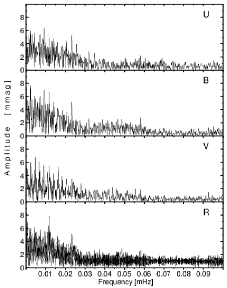
Figure 11: The Fourier amplitude spectra of the Bal09 $UBVR$ observations for frequencies below 0.1 mHz. The data were not detrended, but all terms listed in Tables 1 and 2 were removed.

We see that peaks close to 0 and 1 d^-1 = 11.6 $\mu$Hz appear in all periodograms indicating that some night-to-night changes, presumably of instrumental origin, are present in the data. This can be seen most clearly in the $R$ data. However, there is an indication of a significant peak at frequency of about 9.26 $\mu$Hz or its alias, 11.57 $-$ 9.26 = 2.31 $\mu$Hz in the $U$ and $B$ data. The corresponding periods are equal to 1.25 and 5 days. It is difficult to say whether this is a real periodic change. We think it is rather an artefact caused by transparency changes and/or instrumental effects. The differential combination terms are not visible below 0.1 mHz; they are probably lost in the noise.

3.8 Reality of the detected modes

It is very important from the point of view of the results of this paper to be certain that the modes we detected, especially the low-frequency ones, are real. Moreover, we would like to be certain that they originate in Bal09, and not in the comparison star. In order to verify the latter, we analyzed differential photometry of the comparison star with respect to another star in the field, GSC 02248-00425, called thereafter the check star. Unfortunately, this star is almost 4 mag fainter than the comparison star, so that only the $V$ and $R$ photometry is usable for it. The periodograms of the differential photometry of the comparison star with respect to the check star show no peak above S/N = 3.7 corresponding to the semi-amplitude of 3.0 mmag in $V$ data and no peaks above S/N = 4.1 corresponding to 1.9 mmag in the $R$ data. This justifies that all modes with semi-amplitudes exceeding 2 mmag in $R$ or $3$ mmag in $V$ originate indeed in Bal09. Among them, there are two low-frequency modes, $f_{\rm A}$ and $f_{\rm B}$. We cannot, however, exclude the possibility that some low-frequency modes originate in the comparison star.

An additional argument for the reality of the low-frequency modes may come from an independent detection of a given mode in the data split into two parts; see Kilkenny et al. (1999) for an example. Consequently, we divided the photometry of Bal09 into two, roughly equal parts, before and after HJD 2453254. Then, the analysis of the two parts was performed independently. This was done for data in all four filters. Of 22 independent terms from Table 1, we detected 14 terms in both parts with S/N $>$ 4.5, or 16 if detection threshold was lowered to S/N = 4. The remaining six terms, $f_{\rm F}$, $f_{\rm G}$, $f_{6}$, $f_{7}$, $f_{11}$, and $f_{12}$, were detected in the periodogram of only one part of the data. This does not necessarily mean that these modes are spurious. As a consequence of splitting the data, the noise level increases, masking the low-amplitude modes.

An amplitude change could be another reason for finding a mode in only one half of the data. In order to check this, we compared the semi-amplitudes of the modes derived independently from the two parts of the data, but with the frequencies fixed at the values given in Table 1. The formal rms errors of semi-amplitudes derived from the time-series data similar to our dataset are known to be underestimated by a factor of about two (Handler et al. 2000, Jerzykiewicz et al. 2005; see also Montgomery & O’Donoghue 1999). If we take this into account, denoting the doubled formal rms errors of the semi-amplitudes in a giver filter $i$ by $\varepsilon_{i}$, we may conclude that the differences in semi-amplitudes between the first and the second part of our data exceed 3 $\varepsilon_{i}$ only for $f_{1}$ in $U$ (3.2 $\varepsilon_{\rm U}$), $V$ (4.7 $\varepsilon_{\rm V}$), and $R$ (3.2 $\varepsilon_{\rm R}$), and for $f_{3}$ in $U$ (4.0 $\varepsilon_{\rm U}$) and $V$ (3.5 $\varepsilon_{\rm V}$). For about 70% of filter/mode combinations the differences were smaller than $\varepsilon_{i}$. We may therefore conclude that there are no significant amplitude differences between the two parts of the data except for a marginal change of the amplitude of two modes, $f_{1}$ (increase) and $f_{3}$ (decrease).

4 The amplitudes

A vast majority of the photometric observations of EC 14026 stars was made without any filter. This was a compromise between the required photometric accuracy and the exposure time needed for the very short periodicities observed in these variables. However, the multicolour observations are highly desirable since they can support mode identification, a starting point for successful asteroseismology. The best examples of the multicolour observations of EC 14026 stars made so far are the $UBVR$ data of Koen (1998) for V 2203 Cyg = KPD 2109+4401, the $u^{\prime}g^{\prime}r^{\prime}$ photometry of the same star and V 429 And = HS 0039+4302 = Balloon 84041013 (Jeffery et al., 2004), four-band photometry of V 338 Ser (Falter et al., 2003), and $UBVR$ observations of LM Dra = PG 1618+563B (Silvotti et al., 2000).

Since Bal09 is relatively bright and mode identification is one of the main goals of our study, we observed it through wide-band filters. There is, however, a price. The residual standard deviation of our $UBVR$ observations, a measure of typical accuracy of a single data point, is quite large, and amounts to 0.015, 0.011, 0.010, and 0.010 mag, respectively (Table 1). Fortunately, owing to the large number of the observations we gathered, the detection threshold in Fourier periodograms is reasonably low, 0.8–1.4 mmag.

The semi-amplitudes in all filters are given in Table 1. It is worth noting that, along with the main mode in V 338 Ser (Koen et al., 1998a), the $f_{1}$ mode has the largest amplitude of all modes known in EC 14026 stars. Generally, the semi-amplitudes become smaller towards longer wavelengths as the theory predicts (see, e.g., Ramachandran et al. 2004). For five modes with the largest amplitudes we plot the amplitude ratios in Fig. 12. They are normalized to the $U$-filter amplitude.

Figure 12: Relative amplitudes, $A_{i}/A_{\rm U}$, $i=\{B,V,R\}$, for the five largest-amplitude modes detected in Bal09: $f_{1}$, large filled circles, $f_{2}$, $f_{3}$, $f_{4}$ triplet, open circles, and $f_{8}$, dots. Error bars were calculated from formal errors of semi-amplitudes given (Table 1).

The phase differences (Table 1) are equal to zero within the errors for all modes.

5 Discussion

5.1 Preliminary mode identification

There are at least two possibilities to identify modes solely from the photometry. The first method relies on the comparison of the amplitude ratios and phase differences with those calculated from the model atmospheres for a given mode. The amplitude ratios were already used to constrain degree $\ell$ in EC 14026 stars by Koen (1998) and Jeffery et al. (2004). However, these papers and the theoretical work of Ramachandran et al. (2004) indicate that when going from shorter to longer wavelength in the optical domain, the amplitudes of low-degree ($\ell\leq$ 2) $p$ modes for EC 14026 models behave similarly. Therefore, the $\ell$ for the $\ell\leq$ 2 modes is hardly derivable from amplitude ratios. Modes with $\ell$ = 3 and 4 are much better separated: these with $\ell$ = 3 show rather flat dependence on wavelength, while those with $\ell$ = 4, much steeper than the $\ell\leq$ 2 modes. The amplitude ratios for five modes shown in Fig. 12 exhibit similar change with wavelength as the $\ell\leq$ 2 modes. We may therefore rather safely interpret them as modes having $\ell$ equal to 0, 1 or 2.

The other possibility for mode identification from the photometry is the best match of the observed frequencies to those calculated from the model [Brassard et al. (2001) is a good example]. We make here only a rough comparison of the observed periods with those calculated in the currently available models, giving some indications as to the possible identifications. A detailed mode identification including the stability analysis of models in a wide range of input parameters needs much better modelling and is beyond the scope of this paper; we postpone such a thorough analysis to a separate study.

Let us start with the assumption that the main mode, $f_{1}$, is the radial fundamental one. In addition to the expected wavelength-amplitude ration dependence, the justification for this assumption is its large amplitude. With this assumption, we can go to models in order to try to interpret the other frequencies. A large set of pulsational properties of evolutionary models was published by Charpinet et al. (2002) (hereafter C02) for seven extended horizontal branch (EHB) sequences. All sequences were calculated for a star with mass $\sim$0.48 $M_{\odot}$, but with different envelope masses: 0.0001, 0.0002, 0.0007, 0.0012, 0.0022, 0.0032, and 0.0042 $M_{\odot}$ for sequences 1 to 7, respectively. These models are shown in the $\log T_{\rm eff}$ – $\log g$ diagram in Fig. 13. The position of Bal09, according to the parameters derived by Oreiro et al. (2004), is also shown.

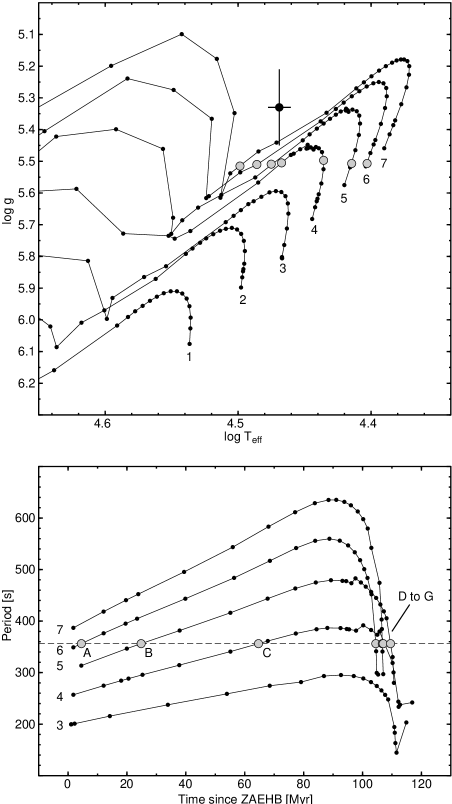
Figure 13: Top: Seven evolutionary sequences (labeled from 1 to 7) showing the extended horizontal branch evolution of a 0.47–0.48 $M_{\odot}$ star, taken from Charpinet et al. (2002). It is mainly the hydrogen envelope mass that differentiate the models; it ranges from 0.0001 $M_{\odot}$ for sequence 1 up to 0.0042 $M_{\odot}$ for sequence 7. The large dot with error bars denotes the parameters of Bal09 as derived by Oreiro et al. (2004). Seven filled gray circles show the position of models A to G for which the period of the fundamental radial mode is equal to 1/$f_{1}$. Bottom: Periods of the fundamental radial mode, $\ell$ = 0, $p_{0}$ for five of the seven evolutionary sequences shown above. The dashed horizontal line corresponts to $P_{1}$ = 1/$f_{1}$ = 356.19 s. Gray filled circles show the positions of the seven models, A to G (see Table 3), that match the period exactly.

C02 provide also the pulsation periods for modes with $\ell$ up to 3. The periods of the fundamental radial mode ($\ell$ = 0, $p_{0}$) are shown for all but the first two sequences in the bottom panel of Fig. 13. The line for $P_{1}$ = 1/$f_{1}$ = 356.19 s intersects the model values in seven points corresponding to seven models belonging to sequences 4 to 7. Their properties, derived from linear interpolation of the model grid of C02, are listed in Table 3. We see that none of the models with envelope mass less than $\sim$0.001 $M_{\odot}$ can be fit with the period of the fundamental radial mode equal to $P_{1}$. The seven models in the sequence from the least evolved to the most evolved we denote with the letters A to G. The A to C models cover the main part of the EHB helium core burning evolution (HeCB in Table 3), D to F, its final stage, and G, the core helium exhaution (CHeE). The models are plotted in Fig. 13 with filled gray circles. Note that regardless of the model, the theoretical value of $\log g\approx$ 5.51 agrees reasonably well with the result of Oreiro et al. (2004).

Table 3: Parameters of interpolated models that have the period of the fundamental radial mode equal to 356.19 s.

Model	C02 model	Age∗	Evol.	$\log T_{\rm eff}$	$\log g$
	sequence	[Myr]	phase
A	6	4.51	HeCB	4.403	5.51
B	5	24.81	HeCB	4.415	5.51
C	4	64.66	HeCB	4.436	5.50
D	4	107.02	end of HeCB	4.467	5.51
E	5	109.51	end of HeCB	4.475	5.51
F	6	104.51	end of HeCB	4.486	5.51
G	7	106.70	CHeE	4.499	5.52

^∗ since ZAEHB.

Having interpolated the models that match exactly $P_{1}$, we can try to compare the other periods as well. This is done in Fig. 14 for all seven models. For clarity, the $\ell$ = 3 modes are not shown in this figure. We see that the observed pattern resembles to some extent the theoretical one (certainly with many high-overtone modes missing). We can therefore derive some conservative conclusions based on this comparison. Since besides the strong 356-s term, we have only three narrow ranges in period where the observed modes occur, we can try to constrain the possible identification.

Figure 14: Comparison of the pulsation periods for models A–G, indicated in Fig. 13, with periods detected in Bal09. For the models, the radial ($\ell$ = 0) modes are shown with continuous lines, $\ell$ = 1 modes with dashed lines, and $\ell$ = 2 modes with dotted lines. See text for more details.

The separation between $f_{1}$ and the central term of the rotationally split triplet ($f_{3}$) is best reproduced by model D. This is also the model with no $\ell\leq$ 2 modes having periods in the range between 270 and 340 s, in accordance with observations. Moreover, model D is closest in $T_{\rm eff}$ to the observed value (Fig. 13). However, we are far from indicating that model D is the best one, and constraining the evolutionary status of Bal09. The problem requires better modelling.

Nevertheless, some indications as to the mode identification can be given even from this simple exercise. The mode closest in period to $p_{0}$, on the short-period side, is in all models the $\ell$ = 1 mode. It has radial order $n$ = 1 for all models but G, where it has $n$ = 2. However, while for the three less evolved models it is the $p_{1}$ mode, it is replaced in period for the remaining, more evolved models, by $g_{1}$ (D–F) or even $g_{2}$ (G) due to the phenomenon of avoided crossing. The $g$ modes under consideration have mixed character and are typical for evolved models also in main-sequence pulsators. An $\ell$ = 1 identification can be therefore attributed with high probability to the rotationally split modes $f_{2}$, $f_{3}$, and $f_{4}$; the azimuthal orders would then be $m$ = $-$1, 0, and +1, respectively.

There is a general trend that for the three groups of periods detected in Bal09, that is, around 350, 260 and 215 s, there are always nearby theoretical modes with $\ell$ = 0, 1 and 2. This can be seen in Fig. 13. In Table 4 we identified the theoretical modes closest to the observed ones for all seven models.

Table 4: Identification of the family ($p,f$ or $g$) and radial order (subscript) of modes with $\ell$ = 0, 1, and 2 closest to each of the three period groups detected in Bal09 for seven models listed in Table 3.

	Period group			Period group			Period group
	350–356 s			263–265 s			214–215 s
Model	$\ell$ = 0	1	2	0	1	2	0	1	2
A, B, C	$p_{0}$	$p_{1}$	$g_{1}$	$p_{1}$	$p_{2}$	$p_{1}$	$p_{2}$	$p_{3}$	$p_{2}$
D	$p_{0}$	$g_{1}$	$g_{1}$	$p_{1}$	$p_{2}$	$f$	$p_{2}$	$p_{3}$	$p_{2}$
E	$p_{0}$	$g_{1}$	$g_{2}$	$p_{1}$	$p_{2}$	$f$	$p_{2}$	$p_{3}$	$p_{1}$
F	$p_{0}$	$g_{1}$	$g_{3}$	$p_{1}$	$p_{1}$	$g_{1}$	$p_{2}$	$p_{3}$	$p_{1}$
G	$p_{0}$	$g_{2}$	$g_{5}$	$p_{1}$	$p_{1}$	$g_{2}$	$p_{2}$	$p_{2}$	$f$

5.2 Coexistence of low and high-frequency modes

There is no doubt that the low-frequency modes, presumably high-order $g$ modes, exist in Bal09. The question arises whether such modes are also present in the other cool and evolved EC 14026 stars. The low-frequency region is sometimes ignored in the frequency analysis and signals, even when found, are frequently attributed to the atmospheric transparency variations or removed during the detrending process. However, high-order $g$ modes discovered so far have periods shorter than 2 hours. Thus, two to four cycles may be covered during a single night and these signals can be easily distinguished from the transparency variations, especially in the differential photometry. It is therefore worthwhile to reanalyze some already existing long data sets with the aim of searching for low-frequency modes. While writing this paper, we have learned about the discovery of a long-period mode in HS 0702+6043 (Schuh et al., 2004). It is worth noting that both Bal09 and HS 0702+6043 are neighbours of the PG 1716+426 group of pulsating subdwarfs in the $\log T_{\rm eff}$ – $\log g$ diagram, and some other EC 14026 stars are close by (V 338 Ser, V 391 Peg and KL UMa). These stars should be considered as primary targets in the search for high-order $g$ modes in EC 14026 stars.

5.3 Frequency splitting

Modes close in frequency were detected in many EC 14026 stars, and some of them were supposed to be rotationally split ones. This would allow estimating rotational periods. However, up to now, the only rotationally split triplet was found in EO Cet = PB 8783 (O’Donoghue et al. 1998). In several other EC 14026 stars only close doublets were found. The equidistant triplet found by us in Bal09 is therefore the second one detected in an EC 14026 star. If we accept that it is a rotationally split $\ell$ = 1 mode (see Sect. 5.1), we can translate the observed mean splitting, $\Delta f$ = 1.58 $\mu$Hz, into the rotation period $P_{\rm rot}=(\mbox{1}-C_{n\ell})/\Delta f$, where $C_{n\ell}$ is the Ledoux constant. For all models considered in previous section but model D, the values of $C_{n\ell}$ provided by C02 lie between 0.01 and 0.04, implying $P_{\rm rot}$ = 7.1 $\pm$ 0.1 d. Only for model D, the $C_{n\ell}$ is higher and can reach 0.2. In that case $P_{\rm rot}$ would be smaller, about 6 d. Bal09 is therefore very likely a slow rotator. The 7.1-day rotation period for a star with a mass of 0.48 $M_{\odot}$ and $\log g$ = 5.51 results in the equatorial rotation velocity of 1.44 km/s.

5.4 Final remarks

It is clear for us that Bal09 is one of the most interesting targets for the future study by means of asteroseismology. The main reason for this is the coexistence of the pulsations inherent to both classes of pulsating sdB stars: the EC 14026 and PG 1716+426 stars. As far as the excited pulsations are concerned, it seems simpler than the best studied EC 14026-type star V 338 Ser that is a fast rotator (Heber et al., 1999). Bal09 rotates slowly and is relatively bright. It is also exceptional because of the presence of a rotationally split mode and the fact that a large number of combination frequencies are detected.

In addition to a better modelling we are going to undertake in near future, the next step in our understanding of Bal09 could be taken if a new photometric and spectroscopic campaign were organized. Such a campaign should at least remove the 1 d^-1 ambiguity of some of the derived frequencies and lower the detection threshold down to 0.1–0.2 mmag. Both these goals could be achieved if the star were observed in several observatories spread over the longitude, preferably in white light (or very wide band filters). Multicolour observations can support mode identification, but we showed in Sect. 4 that the $\ell$ value can be reliably constrained in that way only for the largest-amplitude modes. It seems, anyway, that even with accurate amplitudes it will be hard to disentangle modes with $\ell$ = 0, 1, and 2, and it might be necessary to go to satellite UV to make a significant progress (see Fontaine & Chayer 2004).

The campaign we plan should be supplemented by spectroscopic observations. Some time-resolved spectroscopic observations of EC 14026 stars have been already done. They were, however, usually too short in duration or badly distributed in time to result in a breakthrough in the mode identification. In case of Bal09, however, even confirming that the main frequency, $f_{1}$, corresponds to the radial mode, as we suggested, would be helpful. The best way towards proper identification would come, however, from accurate matching the model frequencies to the observed ones. This is even possible with our results provided that a thorough modelling would be done. As a by-product, stellar parameters of Bal09 could be obtained. As noted above, we postpone this work to a separate paper.

Acknowledgements. The discussions with S. Kawaler, S. O’Toole and P. Moskalik and comments of an anonymous referee are greatly appreciated. We also thank M. Jerzykiewicz for critical reading of the manuscript and G. Kopacki for allowing us to use his calibration programs.

References

- Billères et al. (2000) Billères M., Fontaine G., Brassard P. et al., 2000, ApJ 530, 441
- Billères et al. (2002) Billères M., Fontaine G., Brassard P., Liebert J., 2002, ApJ 578, 515
- Bixler et al. (1991) Bixler J.V., Bowyer S., Laget M., 1991, A&A 250, 370
- Brassard et al. (2001) Brassard P., Fontaine G., Billères M., Charpinet S., Liebert J., Saffer R.A., 2001, ApJ 563, 1013
- Charpinet et al. (1996) Charpinet S., Fontaine G., Brassard P., Dorman B., 1996, ApJ 471, L103
- Charpinet et al. (1997) Charpinet S., Fontaine G., Brassard P. et al., 1997, ApJ 483, L123
- Charpinet et al. (2001) Charpinet S., Fontaine G., Brassard P., 2001, PASP 113, 775
- Charpinet et al. (2002) Charpinet S., Fontaine G., Brassard P., Dorman B., 2002, ApJS 140, 469 (C02)
- Dorman et al. (1995) Dorman B., O’Connell R., Rood R., 1995, ApJ 442, 105
- Dreizler et al. (2002) Dreizler S., Schuh S.L., Deetjen J.L., Edelmann H., Heber U., 2002, A&A 386, 249
- Falter et al. (2003) Falter S., Heber U., Dreizler S., Schuh S.L., Cordes O., Edelmann H., 2003, A&A 401, 289
- Fontaine & Chayer (2004) Fontaine G., Chayer P., 2004, Proc. Astrophysics in the Far Ultraviolet, eds. G. Sonneborn, H.W. Moos & B.-G. Andersson, in press (astro-ph/0411091)
- Fontaine et al. (2003) Fontaine G., Brassard P., Charpinet S. et al., 2003, ApJ 597, 518
- Green et al. (2003) Green E.M., Fontaine G., Reed M.D. et al., 2003, ApJ 583, L31
- Greggio & Renzini (1990) Greggio L., Renzini A., 1990, ApJ 364, 35
- Handler et al. (2000) Handler G., Arentoft T., Shobbrook R.R. et al., 2000, MNRAS 318, 511
- Heber (1986) Heber U., 1986, A&A 155, 33
- Heber et al. (1999) Heber U., Reid I.N., Werner K., 1999, A&A 348, L25
- Jeffery et al. (2004) Jeffery C.S., Dhillon V.S., Marsh T.R., Ramachandran B., 2004, MNRAS 352, 699
- Jerzykiewicz et al. (2005) Jerzykiewicz M., Handler G., Shobbrook R.R. et al., 2005, MNRAS, submitted
- Kilkenny et al. (1997) Kilkenny D., Koen C., O’Donoghue D., Stobie, R.S., 1997, MNRAS 285, 640
- Kilkenny et al. (1999) Kilkenny D., Koen C., O’Donoghue D. et al., 1999, MNRAS 303, 525
- Koen (1998) Koen C., 1998, MNRAS 300, 567
- Koen et al. (1998a) Koen C., O’Donoghue D., Lynas-Gray A.E., Marang F., van Wyk F., 1998a, MNRAS 296, 317
- Koen et al. (1998b) Koen C., O’Donoghue D., Pollacco D.L., Nitta A., 1998b, MNRAS 300, 1105
- Loumos & Deeming (1978) Loumos G.L., Deeming T.J., 1978, Ap&SS 56, 285
- Montgomery & O’Donoghue (1999) Montgomery M.H., O’Donoghue D., 1999, Delta Scuti Star Newsletter 13, 28
- O’Donoghue et al. (1998) O’Donoghue D., Koen C., Solheim J.-E. et al., 1998, MNRAS 296, 296
- Oreiro et al. (2004) Oreiro R., Ulla A., Pérez Hernández F., Østensen R., Rodríguez López C., MacDonald J., 2004, A&A 418, 243
- Østensen et al. (2001a) Østensen R., Solheim J.-E., Heber U., Silvotti R., Dreizler S., Edelmann H., 2001a, A&A 368, 175
- Østensen et al. (2001b) Østensen R., Heber U., Silvotti R., Solheim J.-E., Dreizler S., Edelmann H., 2001b, A&A 378, 466
- Pamyatnykh (1999) Pamyatnykh A.A., 1999, Acta Astron. 49, 119
- Piccioni et al. (2000) Piccioni A., Bartolini C., Bernabei S. et al., 2000, A&A 354, L13
- Ramachandran et al. (2004) Ramachandran B., Jeffery C.S., Townsend R.H.D., 2004, A&A 428, 209
- Reed et al. (2004a) Reed M.D., Kawaler S.D., Zoła S. et al., 2004a, MNRAS 348, 1164
- Reed et al. (2004b) Reed M.D., Green E.M., Callerame K. et al., 2004b, ApJ 607, 445
- Saffer et al. (1994) Saffer R.A., Bergeron P., Koester D., Liebert P., 1994, ApJ 432, 351
- Schuh et al. (2004) Schuh S., Huber J., Green E.M. et al., 2004, Proc. 14th Workshop on White Dwarfs, eds. D. Koester & S. Moehler, in press (astro-ph/0411640)
- Silvotti et al. (2000) Silvotti R., Solheim J.-E., Gonzalez Perez J.M. et al., 2000, A&A 359, 1068
- Silvotti et al. (2002a) Silvotti R., Østensen R., Heber U., Solheim J.-E., Dreizler S., Altmann M., 2002a, A&A 383, 239
- Silvotti et al. (2002b) Silvotti R., Janulis R., Schuh S.L. et al., 2002b, A&A 389, 180
- Stetson (1987) Stetson P.B., 1987, PASP 99, 191
- Ulla et al. (2001) Ulla A., Zapatero Osorio M.R., Pérez Hernández F., MacDonald J., 2001, A&A 369, 986