The effect of a finite mass reservoir on the collapse of spherical isothermal clouds and the evolution of protostellar accretion

Abstract

Motivated by recent observations which detect an outer boundary for starless cores, and evidence for time-dependent mass accretion in the Class 0 and Class I protostellar phases, we reexamine the case of spherical isothermal collapse in the case of a finite mass reservoir. The presence of a core boundary results in the generation of an inward propagating rarefaction wave. This steepens the gas density profile from $r^{-2}$ to $r^{-3}$ or steeper. After a protostar forms, the mass accretion rate $\dot{M}$ evolves through three distinct phases: (1) an early phase of decline in $\dot{M}$, which is a non-self-similar effect due to spatially nonuniform infall in the prestellar phase; (2) for large cores, an intermediate phase of near-constant $\dot{M}$ from the infall of the outer part of the self- similar density profile; (3) a late phase of rapid decline in $\dot{M}$ when accretion occurs from the region affected by the inward propagating rarefaction wave. Our model clouds of small to intermediate size make a direct transition from phase (1) to phase (3) above. Both the first and second phase are characterized by a temporally increasing bolometric luminosity $L_{\rm bol}$, while $L_{\rm bol}$ is decreasing in the third (final) phase. We identify the period of temporally increasing $L_{\rm bol}$ with the Class 0 phase, and the later period of terminal accretion and decreasing $L_{\rm bol}$ with the Class I phase. The peak in $L_{\rm bol}$ corresponds to the evolutionary time when $50\%\pm 10\%$ of the cloud mass has been accreted by the protostar. This is in agreement with the classification scheme proposed by André et al. (Andre93 1993). We show how our results can be used to explain tracks of envelope mass $M_{\rm env}$ versus $L_{\rm bol}$ for protostars in Taurus and Ophiuchus. We also develop an analytic formalism which reproduces the protostellar accretion rate.

1 Introduction

Recent submillimeter and mid-infrared observations suggest that prestellar cores within a larger molecular cloud are characterized by a non-uniform radial gas density distribution (Ward-Thompson et al. WT 1999; Bacmann et al. Bacmann 2000). Specifically, a flat density profile in the central region of size $R_{\rm flat}$ is enclosed within a region of approximately $r^{-1}$ column density profile (and by implication an $r^{-2}$ density profile) of extent $R_{\rm mid}$. Beyond this, a region of steeper density ($\rho\propto r^{-3}$ or greater) is sometimes detected. Finally, at a distance $R_{\rm edge}$, the column density $N$ seems to merge into a background, and fluctuate about a mean value that is typical for the ambient molecular cloud. The first two regions, of extent $R_{\rm flat}$ and $R_{\rm mid}$, respectively, are consistent with models of unbounded isothermal equilibria or isothermal self-similar gravitational collapse (e.g. Chandrasekhar Chandra 1939; Larson Larson 1969; Penston Penston 1969). In either case, the effect of an outer boundary is considered to be infinitely far away (i.e. $R_{\rm mid}\rightarrow\infty$ in our terminology). In numerical simulations of gravitational collapse in which there is a qualitative change in the physics beyond some radius (e.g. a transition from magnetically supercritical to subcritical mass-to-flux ratio: Ciolek & Mouschovias Ciolek93 1993; Basu & Mouschovias Basu94 1994), the development of a very steep outer density profile is also seen. Finally, larger scale simulations of core formation in clouds with uniform background column density (Basu & Ciolek Basu04 2004) show an eventual merger into a near-uniform background column density, demonstrating the existence of $R_{\rm edge}$. The implication of an outer density profile steeper than $r^{-3}$ is that there is a finite reservoir of mass to build the star(s), assuming that the gas beyond $R_{\rm edge}$ is governed by the dynamics and gravity of the parent cloud, and thus does not accrete on to the star(s) formed within the core.

An important constraint of the observations are the actual sizes of the cores. For example, in the clustered star formation regions such as $\rho$ Ophiuchi protocluster, $R_{\rm edge}\la 5000$ AU, and $R_{\rm edge}/R_{\rm flat}\la 5$, while in the more extended cores in Taurus, $5000~{}{\rm AU}\la R_{\rm edge}\la 20000$ AU, and $5\la R_{\rm edge}/R_{\rm flat}\la 10$ (see André et al. Andre 1999; André, Ward-Thompson, & Barsony Andre2 2000). Clearly, only the latter case may approach self-similar conditions.

Once a central hydrostatic stellar core has formed, the mass accretion rate is expected to be constant in isothermal similarity solutions (Shu Shu 1977; Hunter Hunter2 1977; Whitworth & Summers Whit 1985). For example, for the collapse from rest of a singular isothermal sphere (SIS) with density profile $\rho_{\rm SIS}=c_{\rm s}^{2}/(2\pi Gr^{2})$, where $c_{\rm s}$ is the isothermal sound speed, Shu (Shu 1977) has shown that the mass accretion rate ($\dot{M}$) is constant and equal to $0.975\,c^{3}_{\rm s}/G$. However, two effects can work against a constant $\dot{M}$ in more realistic scenarios of isothermal collapse: (1) inward speeds in the prestellar phase are not spatially uniform as in the similarity solutions, and tend to increase inward, meaning that inner mass shells fall in with a greater accretion rate; (2) the effect of a finite mass reservoir will ultimately reduce accretion. The first effect has been clearly documented in a series of papers (e.g. Hunter Hunter2 1977; Foster & Chevalier FC 1993; Tomisaka Tomisaka 1996; Basu Basu97 1997; Ciolek & Königl Ciolek98 1998; Ogino, Tomisaka, & Nakamura Ogino 1999). It is always present since the outer boundary condition for collapse is distinct from the inner limit of self-similar supersonic infall found in the Larson-Penston solution. Rather, the outer boundary condition must represent the ambient conditions of a molecular cloud, which do not correspond to large-scale infall (Zuckerman & Evans Zuck 1974). Additionally, the finite mass reservoir and steeper than $r^{-3}$ profile as a source of the declining accretion rate has been studied analytically by Henriksen, André, & Bontemps (Henriksen 1997) and Whitworth & Ward-Thompson (Whit2 2001), although they did not account for the physical origin of such a steep density slope.

Indeed, a study of outflow activity from young stellar objects (YSO’s) by Bontemps et al. (Bontemps 1996; hereafter BATC) suggests that $\dot{M}$ declines significantly with time during the accretion phase of protostellar evolution. Specifically, BATC have shown that if the CO outflow rate is proportional to $\dot{M}$, then Class 0 objects (young protostars at the beginning of the main accretion phase) have an $\dot{M}$ that is factor of 10 greater (on average) than that of the more evolved Class I objects. In this paper, we investigate in detail how the assumption of constant mass and volume of a gravitationally contracting core can affect the mass accretion rate and other observable properties after the formation of the central hydrostatic stellar core. A very important question is: which of the two effects mentioned above - a gradient of infall speed in the prestellar phase, or a finite mass reservoir and associated steep outer density slope - is more relevant to explaining the observations of BATC? The evolutionary tracks of envelope mass $M_{\rm env}$ versus bolometric luminosity $L_{\rm bol}$ are another important diagnostic of protostellar evolution (André et al. Andre2 2000). BATC have fit the data using a toy model in which $\dot{M}$ decreases with time in exact proportion to the remaining envelope mass $M_{\rm env}$, i.e. $\dot{M}=M_{\rm env}/\tau$, where $\tau$ is a characteristic time.

We seek to explain the observed YSO evolutionary tracks using a physical (albeit highly simplified) model. We perform high resolution one-dimensional spherical isothermal simulations. The initial peak and decline in the mass accretion rate is modeled through numerical simulations and a simplified semi-analytic approach. A second late-time decline in $\dot{M}$ due to a gas rarefaction wave propagating inward from the outer edge of a contracting core, is also studied in detail. Comparisons are made with the observationally inferred decrease of mass accretion rate (BATC), and evolutionary tracks of $M_{\rm env}$ versus bolometric luminosity $L_{\rm bol}$ (from Motte & André Motte 2001).

Numerical simulations of spherical collapse of isothermal cloud cores are described in § 2. The comparison of the model with observations is given in § 3. Our main conclusions are summarized in § 4. An analytical approach for the determination of the mass accretion rate is presented in the Appendix.

2 Isothermal collapse

2.1 Model Assumptions

We consider the gravitational collapse of spherical isothermal (temperature $T=10$ K) clouds composed of molecular hydrogen with a $10\%$ admixture of atomic helium. The models actually represent cloud cores which are embedded within a larger molecular cloud. The evolution is calculated by solving the hydrodynamic equations in spherical coordinates:

$$\frac{\partial\rho}{\partial t}+\frac{1}{r^{2}}\frac{\partial}{\partial r}\left(r^{2}\rho v_{r}\right) = 0$$ (1)

$$\frac{\partial}{\partial t}\left(\rho v_{r}\right)+\frac{1}{r^{2}}\frac{\partial}{\partial r}\left(r^{2}\rho v_{r}v_{r}\right) = -\frac{\partial p}{\partial r}-\rho\frac{G\,M}{r^{2}},$$ (2)

$$\frac{\partial e}{\partial t}+{1\over r^{2}}\frac{\partial}{\partial r}(r^{2}ev_{r}) = -\frac{p}{r^{2}}\frac{\partial}{\partial r}(r^{2}v_{r})$$ (3)

where $\rho$ is the density, $v_{r}$ is the radial velocity, $M$ is the enclosed mass, $e$ is the internal energy density and $p=(\gamma-1)e$ is the gas pressure. The ratio of specific heats is equal to $\gamma=1.001$ for the gas number density $n\leq 10^{11}$ cm^-3, which implies isothermality (the value of $\gamma$ is not exactly unity in our implementation in order to avoid a division by zero). We define the gas number density $n=\rho/m$, where $m=2.33~{}m_{\rm H}$ is the mean molecular mass. When the gas number density in the collapsing core exceeds $10^{11}$ cm^-3, we form the central hydrostatic stellar core by imposing an adiabatic index $\gamma=5/3$. This simplified treatment of the transition to an opaque protostar misses the details of the physics on small scales. Specifically, a proper treatment of the accretion shock and radiative transfer effects is required to accurately predict the properties of the stellar core (see Winkler & Newman Winkler 1980 for a detailed treatment and review of work in this area). However, our method should be adequate to study the protostellar accretion rate, and has been used successfully by e.g. Foster & Chevalier (FC 1993) and Ogino et al. (Ogino 1999) for this purpose. We use the method of finite-differences, with the time-explicit, operator split solution procedure used in the ZEUS-1D numerical hydrodynamics code; it is described in detail by Stone & Norman (Stone 1992). We have introduced the momentum density correction factor, as advocated by Mönchmeyer & Müller (MM 1989), to avoid the development of an anomalous density spike at the origin (see Vorobyov & Tarafdar VT 1999 for details). The numerical grid has 700 points which are initially uniformly spaced, but then move with the gas until the central stellar core is formed. This provides an adequate resolution throughout the simulations.

We impose boundary conditions such that the gravitationally bound cloud core has a constant mass and volume. The assumption of a constant mass appears to be observationally justified by the sharp outer density profiles described in § 1. Physically, this assumption may be justified if the core decouples from the rest of a comparatively static, diffuse cloud due to a shorter dynamical timescale in the gravitationally contracting central condensation than in the external region. A specific example of this, due to enhanced magnetic support in the outer envelope, is found in the models of ambipolar-diffusion induced core formation (see, e.g. Basu & Mouschovias Basu95 1995). The assumption of a constant volume is mainly an assumption of a constant radius of gravitational influence of a cloud core within a larger parent diffuse cloud.

The radial gas density distribution of a self-gravitating cloud with finite central density that is in hydrostatic equilibrium (e.g. Chandrasekhar Chandra 1939) can be conveniently approximated by a modified isothermal sphere, with gas density

$$\rho=\frac{\rho_{\rm c}}{1+(r/r_{c})^{2}}$$ (4)

(Binney & Tremaine BT 1987), where $\rho_{\rm c}$ is the central density and $r_{\rm c}$ is a radial scale length. We choose a value $r_{\rm c}=1.1~{}c_{s}/\sqrt{\pi G\rho_{\rm c}}$, so that the inner profile is close to that of a Bonnor-Ebert sphere, $r_{\rm c}$ is comparable to the Jeans length, and the asymptotic density profile is 2.2 times the equilibrium singular isothermal sphere value $\rho_{\rm SIS}=c_{\rm s}^{2}/(2\pi Gr^{2}$). The latter is justified on the grounds that core formation should occur in a somewhat non-equilibrium manner (an extreme case is the Larson-Penston flow, in which case the asymptotic density profile is as high as $4.4\,\rho_{\rm SIS}$), and also by observations of protostellar envelope density profiles that are often overdense compared to $\rho_{\rm SIS}$ (André, Motte, & Belloche Andre3 2001).

For small radii ($r\leq r_{\rm c}$), the initial density is very close to the equilibrium solution for an isothermal sphere with a finite central density. However, at large radii it is twice the value of the equilibrium isothermal sphere, which converges to $\rho_{\rm SIS}$. Hence, our initial conditions resemble those of other workers (Foster & Chevalier FC 1993; Ogino et al. Ogino 1999) who start with Bonnor-Ebert spheres and add a positive density perturbation in order to initiate evolution. Use of the modified isothermal sphere simplifies the analysis a little bit since there is a clear transition from flat central region to a power-law outer profile. The choice of central density $\rho_{\rm c}$ and outer radius $r_{\rm out}$ determines the cloud mass. We study many different cloud masses - two models are presented in this section and other models are used to fit observational tracks in § 3. We also add a (small) positive density perturbation of a factor of 1.1 (i.e. the initial gas density distribution is increased by a factor of 1.1) to drive the cloud (especially the inner region which is otherwise near-equilibrium) into gravitational collapse.

Table 1 shows the parameters for two model clouds presented in this section. The adopted central number density $n_{\rm c}=5\times 10^{4}$ cm^-3 is roughly an order of magnitude lower than is observed in prestellar cores (Ward-Thompson et al. WT 1999). Considering that these cores may be already in the process of slow gravitational contraction, our choice of $n_{\rm c}$ is justified for the purpose of describing the basic features of star formation. In both models, the outer radius $r_{\rm out}$ is chosen so as to form gravitationally unstable prestellar cores with central-to-surface density ratio $\rho_{\rm c}/\rho_{\rm out}\geq 14$ (since our initial states are similar to Bonnor-Ebert spheres). In model I1, $\rho_{\rm c}/\rho_{\rm out}\approx 24$ and by implication $r_{\rm out}/r_{\rm c}\approx 4.7$, whereas in model I2 $\rho_{\rm c}/\rho_{\rm out}\approx 324$ and $r_{\rm out}/r_{\rm c}\approx 18$. Model I2 thus represents a very extended prestellar core. Models I1 and I2 have masses $5~{}M_{\odot}$ and $24~{}M_{\odot}$ respectively; the ‘I’ stands for isothermal.

Table 1: Model parameters

Model	$n_{\rm c}$	$r_{\rm c}$	$r_{\rm out}$	${\rho_{\rm c}\over\rho_{\rm out}}$	$M_{\rm cl}$	$T$
I1	$5.0$	0.033	0.16	24	5	10
I2	$5.0$	0.033	0.5	324	24	10

All number densities are in units of $10^{4}$ cm^-3, lengths are in pc, masses in $M_{\odot}$, and temperatures in K.

2.2 Numerical Results

Fig. 1 shows the temporal evolution of the radial gas density profiles (the upper panel) and velocity profiles (the lower panel) during the runaway collapse phase (before the formation of the central hydrostatic stellar core) in model I1. The density and velocity profiles are numbered according to evolutionary sequence, starting from the initial distributions (profile 1; note that the cloud core is initially at rest) and ending with those obtained when the central number density has almost reached $10^{10}$ cm^-3 (profile 5). The dashed lines in the upper panel of Fig. 1 show the power-law index $d\ln\rho/d\ln r$ of the gas distribution for profiles 1, 2, and 3. By the time that a relatively mild center-to-boundary density contrast $\sim 150$ is established (profile 2), the radial density profile starts resembling those observed in Taurus by Bacmann et al. (Bacmann 2000): it is flat in the central region, then gradually changes to an $r^{-2}$ profile, and falls off as $r^{-3}$ or steeper in the envelope at $r\ga 0.08$ pc. The sharp change in slope of the density profile (e.g. at $r\sim 0.08$ pc in profile 2 of Fig. 1) is due to an inwardly-propagating gas rarefaction wave caused by a finite reservoir of mass. The self-similar region with $r^{-2}$ density profile is of the Larson-Penston type, with density somewhat greater than the equilibrium singular isothermal sphere value ($c_{\rm s}^{2}/2\pi Gr^{2}$). The velocity profiles in Fig. 1 also show a distinct break at the instantaneous location of the rarefaction wave. Furthermore, the peak infall speed is clearly supersonic (since $c_{\rm s}=0.19$ km s^-1) by the time profile 4 is established, again consistent with Larson-Penston type flow in the inner region.

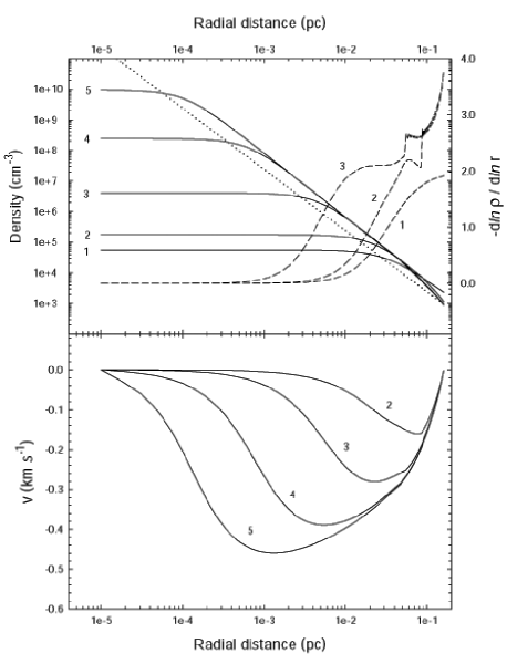
Figure 1: The radial gas density (the upper panel) and velocity (the lower panel) profiles obtained in model I1 before the central hydrostatic stellar core is formed. The number 1 corresponds to the initial profiles (note that initially the cloud core is at rest) and the number 5 labels profiles when the central gas number density has almost reached $10^{10}$ cm^-3. The dashed lines in the upper panel show the power-law index $d\ln\rho/d\ln r$ of the gas distributions 1, 2, and 3. Profiles 2, 3, 4, and 5 are reached at times 0.309 Myr, 0.378 Myr, 0.392 Myr, and 0.394 Myr, respectively. For reference, the dotted line is the density profile of a singular isothermal sphere.

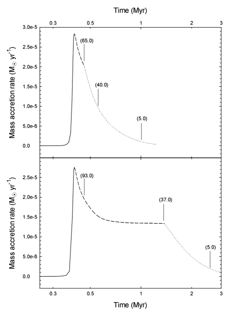
Figure 2: The temporal evolution of the mass accretion rate at the radial distance $r=600$ AU from the center of a cloud core obtained in a) model I1 and b) model I2. The model cloud I1 has mass 5 $M_{\odot}$ and the model cloud I2 has mass 24 $M_{\odot}$. The solid lines show $\dot{M}$ during the runaway collapse phase, prior to the formation of a central stellar core. The dashed and dotted lines plot $\dot{M}$ after stellar core formation; the dashed lines show $\dot{M}$ before the gas affected by the inwardly propagating rarefaction wave has reached $r=600$ AU, whereas the dotted lines show $\dot{M}$ after this gas has reached $r=600$ AU. The numbers in parentheses reflect the percentage of cloud mass remaining in the envelope at the given times.

Fig. 2a shows the temporal evolution of the accretion rate at a radial distance of 600 AU from the center in model I1. The evolution is characterized by a slow initial gravitational contraction and then a very rapid increase until about 0.4 Myr. Subsequently, a central hydrostatic stellar core forms and the mass accretion rate reaches its maximum value of $2.8\times 10^{-5}~{}M_{\odot}$ yr^-1 (or $17.4~{}c_{\rm s}^{3}/G$). After stellar core formation, the evolution of the mass accretion rate has possibly three distinct phases, of which two are on display in Fig. 2a. The early phase, plotted with the dashed line in Fig. 2a, is characterized by accretion of material that has not yet been affected by the rarefaction wave propagating inward from the outer boundary. The accretion rate is declining, even though the density profile near the stellar core was nearly self-similar at the moment of its formation. This decline is due to the gradient of infall velocity in the inner regions, an effect not predicted in the similarity solutions. However, if there is a large outer region with mass shells that are falling in at significantly subsonic speeds when the central stellar core forms (see discussion of Fig.  2b below), the accretion rate will eventually stabilize to a constant value that is consistent with the standard theory of Shu (Shu 1977). In that picture, progressively higher shells of gas lose their partial pressure support and start falling from rest on to the central stellar core almost in a free-fall manner. This would be the intermediate phase of accretion. However, the late phase of very rapid decline of the accretion rate starts at roughly 0.46 Myr (before the intermediate phase can be established in the $5\,M_{\odot}$ cloud), when gas affected by the inwardly propagating rarefaction wave reaches the inner 600 AU. This results in a sharp drop of $\dot{M}$ as shown in Fig. 2a by the dotted line.

The existence of the (in principle) three distinct phases of mass accretion is clearly seen Fig. 2b, where $\dot{M}$ of the more extended cloud ($r_{\rm out}/r_{\rm c}\approx 18$) is plotted (hereafter, model I2). The outer boundary is now at $r_{\rm out}=0.5$ pc and it takes a time $\ga 1$ Myr for the influence of the rarefaction wave to reach the inner 600 AU. As a result, the mass accretion rate has time to stabilize at a constant value of $1.34\times 10^{-5}~{}M_{\odot}$ yr^-1 (the dashed line in Fig. 2b), before it sharply drops at later times (the dotted line in Fig. 2b). According to Shu (Shu 1977), the collapse from rest of a power-law profile that has a density equal to twice $\rho_{\rm SIS}$ yields a mass accretion rate $5.58\,c_{\rm s}^{3}/G=8.86\times 10^{-6}~{}M_{\odot}$ yr^-1. Our stable intermediate accretion rate is roughly consistent with this prediction since the density in the power-law tail is actually somewhat greater than twice $\rho_{\rm SIS}$. It is equal to 2.42 $\rho_{\rm SIS}$ in the initial state, and grows to greater overdensities in the innermost regions. However, the bulk of the matter, which is in the outer tail, has density within $2.5\rho_{\rm SIS}$. Further experiments with our numerical simulations show that the intermediate phase of constant accretion rate is observed only in rather extended prestellar cores with $r_{\rm out}/r_{\rm c}\ga 15$. Foster & Chevalier (FC 1993) found an even stronger criterion $r_{\rm out}/r_{\rm c}\ga 20$. Since more extended cores tend to be more massive as well, we may expect to observe the intermediate phase more frequently in the collapse of massive cores.

2.3 Effect of Boundary Condition

Our standard simulation does not contain an external medium explicitly. In order to explore the effect of such a medium, we ran additional simulations in which the cloud core is surrounded by a spherical shell of diffuse (i.e. non-gravitating) gas of constant temperature and density. The outermost layer of the cloud core and the external gas are initially in pressure balance. We found that the value of $\dot{M}$ in the late accretion phase may depend on the assumed values of the external density and temperature. For instance, if the gravitating core is nested within a larger diffuse non-gravitating cloud of $T=10$ K and $\rho=\rho_{\rm out}$, the accretion rate increases slightly as compared to that shown in Fig. 2 by the dotted line. A warmer external non-gravitating environment of $T=200$ K and $\rho=\rho_{\rm out}/20$ shortens the duration of the late accretion phase shown in Fig. 2 by the dotted line. This phase may be virtually absent if the sound speed of the external diffuse medium is considerably higher (by a factor $\sim 1000$) than that of the gravitationally bound core. This essentially corresponds to a constant outer pressure boundary condition (see Foster & Chevalier FC 1993). However, such a high sound speed contrast is not expected for star formation taking place in a dense ($n\sim 10^{4}$ cm^-3) environment like $\rho$ Ophiuchi (Johnstone et al. Johnstone 2000).

We believe that the constant volume boundary condition, and resulting inward propagating rarefaction wave, are best at reproducing the steep outer density profiles and the low (residual) mass accretion rate necessary to explain the Class I phase of protostellar accretion.

2.4 Semi-analytic Model

Finally, we compute $\dot{M}$ of a pressure-free cloud using the analytical approach developed in the Appendix. This approach allows for the determination of $\dot{M}$ for a cloud with given initial radial density $\rho(r_{\rm 0})$ and velocity $v_{\rm 0}(r_{\rm 0})$ profiles, if the subsequent collapse is pressure-free. We find that the success or failure of the analytical approach to describe the mass accretion rate of the isothermal cloud depends on the adopted $\rho(r_{\rm 0})$ and $v_{\rm 0}(r_{\rm 0})$ profiles. For instance, if $\rho(r_{\rm 0})$ is determined by profile 2 (the upper panel of Fig. 1) and $v_{\rm 0}(r_{\rm 0})=0$, the pressure-free mass accretion rate shown in Fig. 3 by the dashed line reproduces only very roughly the main features of the isothermal accretion rate (the solid line in Fig. 3). However, if we take into account the non-zero and non-uniform velocity profile $v_{\rm 0}(r_{\rm 0})$ plotted in the lower panel of Fig. 1 (profile 2), then the pressure-free $\dot{M}$ shown by the dotted line in Fig. 3 reproduces that of the isothermal cloud much better. This example demonstrates the importance of the velocity field prior to stellar core formation in determining the accretion rates after its formation. The success of our analytical pressure-free approach also shows that the collapse of the isothermal cloud can be regarded as essentially pressure-free from the time of a relatively mild central concentration $\rho_{\rm c}/\rho_{\rm out}\ga 150$, when the central number density $\sim 2\times 10^{5}$ cm^-3.

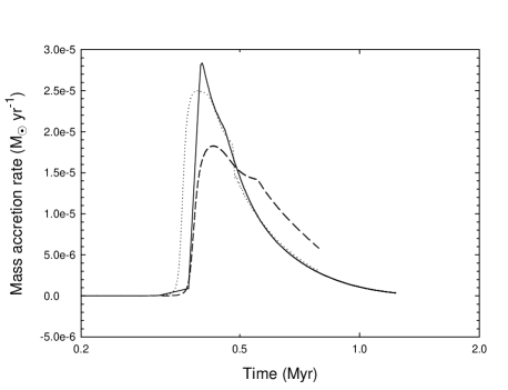
Figure 3: The temporal evolution of the mass accretion rate. The solid line shows the results of isothermal numerical simulations (model I1). The dashed line shows $\dot{M}$ obtained in a pressure-free approximation if such collapse begins from rest with the relatively mildly concentrated density profile 2 in Fig. 1. The dotted line shows the result for pressure-free collapse if a non-zero initial velocity (that of profile 2 in the bottom panel of Fig. 1) is also used. The agreement of the pressure-free model and full numerical simulation are quite good in the latter case.

3 Astrophysical implications

Class 0 objects represent a very early phase of protostellar evolution (see André et al. Andre2 2000), as evidenced by a relatively high ratio of submillimeter luminosity to bolometric luminosity: $L_{\rm submm}/L_{\rm bol}>0.5\%$. Class 0 objects also drive powerful collimated CO outflows. A study of outflow activity in low-mass YSO’s by BATC suggests that the CO momentum flux $F_{\rm co}$ declines significantly during protostellar evolution. Specifically, $F_{\rm co}$ decreases on average by more than an order of magnitude from Class 0 to Class I objects. This tendency is illustrated in Fig. 4, where we plot $F_{\rm co}$ versus $M_{\rm env}$ for 41 sources listed in BATC. We relate $F_{\rm co}$ to $\dot{M}$ by

$$F_{\rm co}=f_{\rm ent}\times(\dot{M}_{\rm w}/\dot{M})V_{\rm w}\times\dot{M},$$ (5)

where $f_{\rm ent}$ is the entrainment efficiency that relates $F_{\rm co}$ to the momentum flux $\dot{M}_{\rm w}V_{\rm w}$ of the wind. Based on theoretical models in the literature, BATC suggested that the factor $f_{\rm ent}$ and the outflow driving engine efficiency $(\dot{M}_{\rm w}/\dot{M})V_{\rm w}$ do not vary significantly during protostellar evolution. This implies that the observed decline of $F_{\rm co}$ reflects a corresponding decrease in $\dot{M}$ from the Class 0 to the Class I stage. Following BATC, we take $f_{\rm ent}=1$, $\dot{M}_{\rm w}/\dot{M}=0.1$, and $V_{\rm w}=150$ km s^-1 and use equation (5) to compute $F_{\rm co}$ from our model’s known mass accretion rate $\dot{M}$ (see Fig. 2).

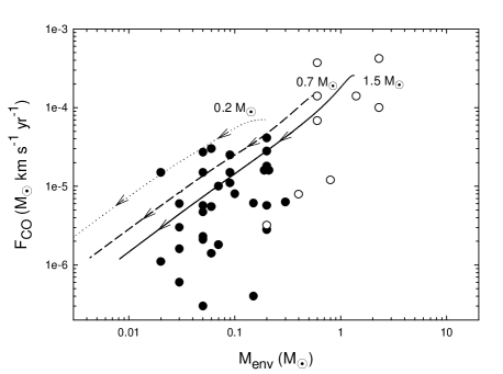
Figure 4: CO momentum flux $F_{\rm co}$ versus envelope mass $M_{\rm env}$ for 41 sources of Bontemps et al. (1996). The Class 0 and Class I objects are plotted with the open and filled circles, respectively. The model $F_{\rm co}-M_{\rm env}$ tracks of three prestellar clouds of $M_{\rm cl}=0.2~{}M_{\odot}$, $0.7~{}M_{\odot}$, and $2~{}M_{\odot}$ are shown by the dotted, dashed, and solid lines, respectively.

Since the sample of Class 0 and Class I objects listed in BATC includes sources from both the Ophiuchus and Taurus star forming regions, we develop model clouds which take into account the seemingly different initial conditions of star formation in these regions. As mentioned in § 1, the two most prominent differences between these two regions are: (1) The cores in Ophiuchus have outer radii ($r_{\rm out}\la 5000$ AU) which are smaller than in Taurus, where $5000~{}{\rm AU}~{}\la~{}r_{\rm out}~{}\la~{}20000$ AU (André et al. Andre 1999; André et al. Andre2 2000); (2) The radial column density profiles of the protostellar envelopes of Class 0 objects in Ophiuchus are at least 2-3 times denser than a SIS at $T=10$ K, whereas in Taurus the protostellar envelopes are overdense compared to the SIS by a smaller factor $\la 2$ (André et al. Andre3 2001). This implies that radial column density profiles of prestellar cores in Ophiuchus and Taurus may follow the same tendency. We develop a set of Ophiuchus model cores which have $r_{\rm out}\la 5000$ AU, and a set of Taurus model cores which have $5000~{}{\rm AU}~{}\la~{}r_{\rm out}~{}\la~{}20000$ AU. Furthermore, the factor $\alpha$ (by which our model density profiles are asymptotically overdense compared to $\rho_{\rm SIS}$) is taken to be $\ga 2.0$ for Ophiuchus and $<2.0$ for Taurus. Clearly, there is no unique set of model cloud parameters that would be exclusively consistent with the observational data, given the measurement uncertainties. We have chosen a set of core central densities $\rho_{\rm c}$, radii $r_{\rm out}$, and overdensity factors $\alpha$ so as to reasonably reproduce the observed properties of the cores in the two regions. The parameters of the model density distributions for Ophiuchus and Taurus are listed in Table 2 and Table 3, respectively.

We also note that we have ensured that the cores satisfy the gravitational instability criterion $r_{\rm out}/r_{\rm c}\ga 3.6$, which is similar to that for Bonnor-Ebert spheres. The Ophiuchus model cores are clustered near this limiting value of $r_{\rm out}/r_{\rm c}$, but the Taurus model cores are allowed to be somewhat more extended, again in keeping with observed properties. We also note that the masses of prestellar cores with the radial density profile given by equation (4) scale as $1/\rho_{\rm c}^{0.5}$, if the ratio $r_{\rm out}/r_{\rm c}$ is fixed.

Table 2: Model parameters for Ophiuchus

$M_{\rm cl}$	$n_{\rm c}$	$r_{\rm out}$	$\rho_{\rm c}/\rho_{\rm out}$	$r_{\rm out}/r_{\rm c}$	$\alpha$
0.17	$1\times 10^{7}$	1600	15.0	3.7	2.0
0.23	$5\times 10^{6}$	1900	14.1	3.6	2.0
0.55	$2\times 10^{6}$	4000	18.0	4.1	2.4
0.9	$2\times 10^{6}$	4000	18.0	4.1	4.0

All number densities are in cm^-3, lengths in AU, and masses in $M_{\odot}$.

Table 3: Model parameters for Taurus

$M_{\rm cl}$	$n_{\rm c}$	$r_{\rm out}$	$\rho_{\rm c}/\rho_{\rm out}$	$r_{\rm out}/r_{\rm c}$	$\alpha$
0.46	$1.5\times 10^{6}$	5000	18	4.1	1.9
0.65	$1\times 10^{6}$	6000	26	5.0	1.8
1.0	$1\times 10^{6}$	10000	71	8.4	1.5
1.5	$8\times 10^{5}$	12000	73	8.5	1.8

All number densities are in cm^-3, lengths in AU, and masses in $M_{\odot}$.

The sample of 41 sources in BATC contains Class 0 and Class I objects from both Ophiuchus and Taurus. Hence, in Fig. 4 we take three representative prestellar clouds of $M_{\rm cl}=0.23~{}M_{\odot}$ (Ophiuchus), $0.65~{}M_{\odot}$ (Taurus), and $2.0~{}M_{\odot}$ (Taurus), for which the $F_{\rm co}-M_{\rm env}$ tracks are shown by the dotted, dashed, and solid lines, respectively. Both the data and model tracks show a near-linear correlation between $F_{\rm co}(\propto\dot{M})$ and $M_{\rm env}$. A slightly better fit of the model tracks to the data can be obtained by adjusting one or more of the estimated parameters $f_{\rm ent}$, $\dot{M}_{\rm w}/\dot{M}$, and $V_{\rm w}$ by factors of order unity.

Based on the near-linear correlation of $F_{\rm co}$ and $M_{\rm env}$, BATC developed a toy model in which $\dot{M}$ decreases with time in exact proportion to the remaining envelope mass $M_{\rm env}$, i.e. $\dot{M}=M_{\rm env}/\tau$, where $\tau$ is a characteristic time. Furthermore, if one assumes that the bolometric luminosity derives entirely from the accretion on to the hydrostatic stellar core, i.e., $L_{\rm bol}=GM_{\rm c}\dot{M}/R_{\rm c}$, where $M_{\rm c}$ and $R_{\rm c}$ are the mass and radius of the stellar core, respectively, then the bolometric luminosity reaches a maximum value when half of the initial prestellar mass has been accreted by the protostar and the other half remains in the envelope. The evolutionary time when $M_{\rm c}=M_{\rm env}$ was defined by André et al. (Andre93 1993) as the conceptual border between the Class 0 and Class I evolutionary stages.

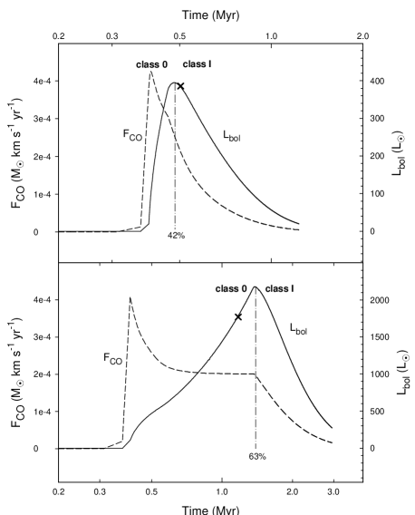
Figure 5: Temporal evolution of the bolometric luminosity $L_{\rm bol}$ and CO momentum flux $F_{\rm co}$. a) The solid and dashed lines show $L_{\rm bol}$ and $F_{\rm co}$ obtained in model I1, respectively. b) The solid and dashed lines show $L_{\rm bol}$ and $F_{\rm co}$ obtained in model I2, respectively. Note that $L_{\rm bol}$ is still increasing during the early phase of accretion rate decline but only declines later due to the more severe accretion rate decline caused by the inward propagating rarefaction wave. The vertical dash-dotted line is the temporal dividing line between the Class 0 and Class I phases for each model; the numbers below give the mass of the central stellar core as a percentage of the total cloud mass. Crosses indicate the time when 50% of the initial cloud mass has been accreted by the protostar. Note the use of a logarithmic scale for time, so that the Class I phase is still longer than the Class 0 phase for model I2.

The solid and dashed lines in Fig. 5a and Fig. 5b show $L_{\rm bol}$ and $F_{\rm co}$ obtained in model I1 and model I2, respectively. Since we do not follow the evolution of a protostar to the formation of the second (atomic) hydrostatic core, we take $R_{\rm c}=3~{}R_{\odot}$ and let $L_{\rm bol}=GM_{\rm c}\dot{M}/R_{\rm c}$. The radius $R_{\rm c}$ depends on the accretion rate and stellar mass (see Fig. 7 of Stahler Stahler 1988) and may vary from $R_{\rm c}\approx 1.5~{}R_{\odot}$ for small stellar cores $M_{\rm c}\sim 0.2~{}M_{\odot}$ and low accretion rates $\dot{M}\sim 2\times 10^{-6}~{}M_{\odot}$ yr^-1 to $R_{\rm c}\approx 5.0~{}R_{\odot}$ for large stellar cores $M_{\rm c}\sim 1.0~{}M_{\odot}$ and high accretion rates $\dot{M}\sim 1\times 10^{-5}~{}M_{\odot}$ yr^-1. However, this variation constitutes roughly a factor of 2 change in the adopted average value of $R_{\rm c}=3~{}R_{\odot}$. Indeed, we performed numerical simulations with a varying $R_{\rm c}$ (assuming a normal deuterium abundance) and found that it has only a minor qualitative influence on our main results. The stellar core mass $M_{\rm c}$ is computed by summing up the masses of the central hydrostatic spherical layers in our numerical simulations. An obvious difference in the temporal evolution of $F_{\rm co}$ and $L_{\rm bol}$ is seen in Fig. 5. The temporal evolution of $F_{\rm co}$ after the central hydrostatic core formation at $t\approx 0.4$ Myr goes through the same phases as shown for $\dot{M}$ in Fig. 2. The temporal evolution of $L_{\rm bol}$ shows two distinct phases: it increases during the early phase (unlike $F_{\rm co}$) and starts decreasing only when gas affected by the inward propagating rarefaction wave reaches the central hydrostatic core. Thus, in our model, only the rarefaction wave acts to reduce $L_{\rm bol}$ during the accretion phase of protostellar evolution. This is a physical explanation for the peak in $L_{\rm bol}$ that also occurs in the toy model of BATC. In that model, the bolometric luminosity reaches a maximum value when exactly half of the initial prestellar mass has been accreted by the protostar. In our simulations, the peak in $L_{\rm bol}$ corresponds to the evolutionary time when $50\%\pm 10\%$ of the matter is in the protostar (higher deviations up to $+15\%$ are found in very massive and extended prestellar clouds).

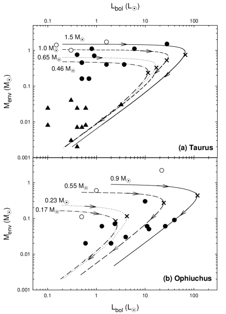
Figure 6: Envelope mass $M_{\rm env}$ versus bolometric luminosity $L_{\rm bol}$ for 37 protostellar objects taken from Motte & André (2001). Diagrams are shown for a) Taurus, and b) Ophiuchus. The Class 0 and Class I objects are plotted with the open and filled circles, respectively. The triangles represent the observed peculiar Class I sources. The model $M_{\rm env}-L_{\rm bol}$ tracks of eight prestellar clouds with masses $M_{\rm cl}=1.5~{}M_{\odot}$, $1.0~{}M_{\odot}$, $0.65~{}M_{\odot}$, and $0.46~{}M_{\odot}$ (Taurus) and $0.9~{}M_{\odot}$, $0.55~{}M_{\odot}$, $0.23~{}M_{\odot}$, and $0.17~{}M_{\odot}$ (Ophiuchus) are shown by the solid, dashed, dotted, and dotted-dashed lines, respectively. Crosses indicate the time when $50\%$ of the cloud mass has been accreted by the protostar.

Finally, in Fig. 6 we show the $M_{\rm env}-L_{\rm bol}$ evolutionary tracks. We use eight representative prestellar cloud core masses as listed in Table 2 and Table 3. Fig. 6a shows the overlaid data for YSO’s in Taurus, while Fig. 6b has overlaid data for Ophiuchus. The data for both samples are taken from Motte & André (Motte 2001). The open circles represent bonafide Class 0 objects, the solid circles represent the bonafide Class I objects, while the triangles represent the so-called peculiar Class I objects observed in Taurus. We note that the envelope masses given in Table 2 of Motte & André (Motte 2001) and plotted in their Fig. 5 and Fig. 6 are determined within a 4200 AU radius circle. While this should relatively well describe the total envelope masses in Ophiuchus, a substantial (a factor of 3) portion of the envelope mass may be missing in the Taurus cores, which have sizes as large as 15000-20000 AU. For this reason, we plot in Fig. 6a the total envelope masses given in Table 4 of Motte & André (Motte 2001) for a set of resolved Taurus cores.

The loci of maximum $L_{\rm bol}$ in the $M_{\rm env}-L_{\rm bol}$ tracks roughly separate two phases in the evolution of a protostar: a shorter one characterized by accretion of matter from the envelope not yet affected by the rarefaction wave (i.e. characterized by the $r^{-2}$ gas density profile or shallower) and a longer one characterized by accretion of matter from the rarefied envelope (i.e. characterized by the $r^{-3}$ profile or steeper). The turnover also corresponds to the evolutionary time when $50\%\pm 10\%$ of the matter is in the protostar and a corresponding amount remains in the envelope as shown by the crosses in Fig. 6. This is in agreement with the observational requirements and toy model of BATC. Given that the peak in $L_{\rm bol}$ is our conceptual dividing line between two distinct phases of accretion, we conclude that in Taurus, most of the so-called Class I objects would tend to fall into the Class 0 category in our scheme. They may indeed be more evolved than the already identified Class 0 objects, having lower values of $\dot{M}$ and $M_{\rm env}$, but would not be in a qualitatively distinct phase of evolution (see Motte & André Motte 2001 for a similar conclusion). In contrast, the so-called peculiar Class I objects in Taurus would be proper Class I objects in our scheme since they are likely in a phase of declining $L_{\rm bol}$. In Ophiuchus, the currently identified Class 0 and Class I objects do seem to fall on two distinct sides of the peak in $L_{\rm bol}$.

Fig. 5 indicates that in extended clouds (as of model I2) the phase of increasing $L_{\rm bol}$ is longer than in compact clouds (as of model I1). This may explain why this phase is more populated in Taurus than in Ophiuchus. In addition, extended clouds have a longer phase of accretion from the envelope not yet affected by the rarefaction wave and, as a consequence, a higher probability of having a quasi-constant accretion phase. This is in agreement with the previous suggestions made by Henriksen et al. (Henriksen 1997) and André et al. (Andre2 2000) that the accretion history in Taurus is closer to the SIS scenario than in Ophiuchus. However, we note that none of our representative prestellar cores listed in Table 3 and used to fit the data for Taurus are extended enough ($r_{\rm out}/r_{\rm c}\ga 15$) to have a distinct phase of constant accretion.

One problem should be pointed out here. While our model $L_{\rm bol}-M_{\rm env}$ tracks in Fig. 6 explain well the measured bolometric luminosities in Ophiuchus, they seem to overestimate $L_{\rm bol}$ in Taurus by a factor of 5-10. This is the so-called “luminosity problem” that was first noticed by Kenyon, Calvet, & Hartmann (Kenyon 1993). As a consequence, the position near the turnover in $L_{\rm bol}-M_{\rm env}$ tracks for Taurus is scarcely populated. This implies that while spherical collapse models may be appropriate for the determination of $L_{\rm bol}$ in Ophiuchus, they tend to overestimate $L_{\rm bol}$ in Taurus. It is possible that a significant magnetic regulation of the early stages of star formation in Taurus, as implied by e.g. polarization maps (Moneti et al. Moneti 1984) would yield more flattened envelopes which result in a lower accretion rate on to the central protostar and a smaller bolometric luminosity. Interestingly, Kenyon et al. (Kenyon 1993) also concluded that envelopes in Taurus should be highly flattened in order to explain their spectral energy distribution. Two dimensional simulations are required to address this issue.

Finally, it is worth noting that our Taurus model cores are generally more massive than the Ophiuchus model cores. This in agreement with observations, and can be justified theoretically on the basis of a lower mean column density (hence greater Jeans length and Jeans mass of a sheetlike configuration) in Taurus compared to regions of more clustered star formation in e.g. Ophiuchus and Orion. Taken at face value, our models then imply that Taurus protostars should be more massive in general than Ophiuchus protostars. While such a conclusion must be tempered by the fact that we do not model magnetic support or feedback from outflows, there is some evidence that Taurus does have a significantly higher mass peak in its initial mass function than does the Trapezium cluster in Orion (see Luhman Luhman 2004 and references within).

4 Conclusions

Our numerical simulations indicate that the assumption of a finite mass reservoir of prestellar cores is required to explain the observed Class 0 to Class I transition. We start our collapse calculations by perturbing a modified isothermal sphere profile (eq. [4]) that is truncated and resembles a bounded isothermal equilibrium state. Specifically, we find that

$\bullet$ Starting in the prestellar runaway collapse phase, a shortage of matter developing at the outer edge of a core generates an inward propagating rarefaction wave that steepens the radial gas density profile in the envelope from $r^{-2}$ to $r^{-3}$ or even steeper.

$\bullet$ After a central hydrostatic stellar core has formed, and the cloud core has entered the accretion phase, the mass accretion rate $\dot{M}$ on to the central protostar can be divided into three possible distinct phases. In the early phase, $\dot{M}$ decreases due to a gradient of infall speed that developed during the runaway collapse phase (such a gradient is not predicted in isothermal similarity solutions). An intermediate phase of near-constant $\dot{M}$ follows if the core is large enough to have an extended zone of self-similar density profile with relatively low infall speed during the prestellar phase. Finally, when accretion occurs from the region affected by the inward propagating rarefaction wave, a terminal and rapid decline of $\dot{M}$ occurs.

$\bullet$ A pressure-free analytic formalism for the mass accretion rate can be used to predict the mass accretion rate after stellar core formation, given the density and velocity profiles in a suitably late part of the runaway collapse phase. Our formulas can estimate $\dot{M}$ at essentially any radial distance from the central singularity. This makes it possible to obtain $\dot{M}$ as a function of radial distance at any given time. We have demonstrated the importance of the velocity field of a collapsing cloud in determining $\dot{M}$; our approach successfully estimates the accretion rate if the velocity field is taken into account. It demonstrates that the initial decline in $\dot{M}$ is due to the gradient of infall speed in the prestellar phase.

$\bullet$ From an observational point of view, we can understand evolutionary $M_{\rm env}-L_{\rm bol}$ tracks using core models of relatively small mass and size, so that there is not an extensive self-similar region, in agreement with the profiles observed by e.g. Bacmann et al. (Bacmann 2000). This means that in the accretion phase, $\dot{M}$ makes a direct transition from the early decline phase to the late decline phase when matter is accreted from the region of steep ($r^{-3}$ or steeper) density profile that is affected by the inward propagating rarefaction wave. In the first phase (which we identify as the true Class 0 phase), the bolometric luminosity $L_{\rm bol}$ is increasing with time, even though $\dot{M}$ and the CO momentum flux $F_{\rm co}$ are slowly decreasing. In the second phase (which we identify as the Class I phase), both $L_{\rm bol}$ and $F_{\rm co}$ decline with time. Hence, our simulations imply that the influence of the rarefaction wave roughly traces the conceptual border between the Class 0 and Class I evolutionary stages. Regions of star formation with more extended cores, like Taurus, should reveal a larger fraction of protostars in the phase of increasing $L_{\rm bol}$. Our Fig. 6 reveals that this is indeed the case, if most of the so-called Class I objects in Taurus are reclassified as Class 0, according to our definition. The so-called peculiar Class I objects in Taurus would be bona-fide Class I objects according to our definition (see Motte & André Motte 2001 for a similar conclusion on empirical grounds).

$\bullet$ Luminosities derived entirely from the accretion on to the hydrostatic stellar core tend to be larger than the measured bolometric luminosities $L_{\rm bol}$ in Taurus by a factor of 5-10, while they seem to better explain the measured $L_{\rm bol}$ in Ophiuchus. This implies that physical conditions in Ophiuchus may favour a more spherically symmetric star formation scenario.

Our results should be interpreted in the context of models of one-dimensional radial infall. They illuminate phenomena which are not included in standard self-similar models of isothermal spherical collapse, by clarifying the importance of boundary (edge) effects in explaining the observed $F_{\rm co}-M_{\rm env}$ and $M_{\rm env}-L_{\rm bol}$ tracks. Important theoretical questions remain to be answered, such as the nature of the global dynamics of a cloud which could maintain a finite mass reservoir for a core. A transition to a magnetically subcritical envelope may provide the physical boundary that we approximate in our model. For example, Shu, Li, & Allen (2004) have recently calculated the (declining) accretion rate from a subcritical envelope on to a protostar, under the assumption of flux freezing. An alternate or complementary mechanism of limiting the available mass reservoir is the effect of protostellar outflows.

Our main observational inference is that a finite mass reservoir and the resulting phase of residual accretion is necessary to understand the Class I phase of protostellar evolution. Our calculated mass accretion rates really represent the infall onto an inner circumstellar disk that would be formed due to rotation. Hence, our results are relatable to observations if matter is cycled through a circumstellar disk and on to a protostar rapidly enough so that the protostellar accretion is at least proportional to the mass infall rate on to the disk. This is likely, since disk masses are not observed to be greater than protostellar masses, but needs to be addressed with a more complete model. In future papers, we will investigate the role of non-isothermality (using detailed cooling rates due to gas and dust), rotation, magnetic fields, and non-axisymmetry in determining $\dot{M}$ and implied observable quantities.

Appendix A Pressure-Free Collapse

A.1 Collapse from rest

The equation of motion of a pressure-free, self-gravitating spherically symmetric cloud is

$${dv\over dt}=-{GM(r)\over r^{2}},$$ (6)

where $v$ is the velocity of a thin spherical shell at a radial distance $r$ from the center of a cloud, and $M(r)$ is the mass inside a sphere of radius $r$. equation (6) can be integrated to yield the expression for velocity $v$

$$v={dr\over dt}=-\sqrt{2GM(r_{\rm 0})\left[{1\over r}-{1\over r_{\rm 0}}\right]},$$ (7)

where $r_{\rm 0}$ is the initial position of a mass shell at $t=0$, and $M(r_{\rm 0})$ is the mass inside $r_{\rm 0}$. Here, it is assumed that all shells are initially at rest: $v_{\rm 0}(r_{\rm 0})=0$. Equation (7) can be integrated by means of the substitution $r=r_{\rm 0}\cos^{2}\beta$ (see Hunter Hunter 1962) to determine the time it takes for a shell located initially at $r_{\rm 0}$ to move to a smaller radial distance $r$ due to the gravitational pull of the mass $M(r_{\rm 0})$. The answer is

$$t={\arccos{\sqrt{r/r_{\rm 0}}}+0.5\sin(2\arccos{\sqrt{r/r_{\rm 0}}})\over\sqrt{2GM(r_{\rm 0})/r^{3}_{\rm 0}}}.$$ (8)

The velocity $v(r,t)$ at a given radial distance $r$ and time $t$ can now be obtained from equations (7) and (8). The values of $r$ and $t$ are sufficient to determine $r_{0}$ (a value $>r$ but $\leq r_{\rm out}$, where $r_{\rm out}$ is the radius of a cloud) from equation (8). Subsequently, we use the obtained value of $r_{0}$ in equation (7) to obtain $v(r,t)$.

Provided that the shells do not pass through each other (i.e. the mass of a moving shell is conserved, $dM(r,t)=dM(r_{0},t_{0})$), the gas density of a collapsing cloud is

$$\rho(r,t)={\rho_{\rm 0}(r_{\rm 0})\>r^{2}_{\rm 0}\>dr_{\rm 0}\over r^{2}\>dr},$$ (9)

where $\rho_{\rm 0}(r_{\rm 0})$ is the initial gas density at $r_{\rm 0}$. The ratio of $dr_{\rm 0}/dr$ determines how the thickness of a given shell evolves with time. The relative thickness $dr_{\rm 0}/dr$ is determined by differentiating $r=r_{\rm 0}\cos^{2}\beta$ with respect to $r_{\rm 0}$, yielding

$${dr\over dr_{\rm 0}}={r\over r_{\rm 0}}-r_{\rm 0}\sin{\left(2\arccos\sqrt{r\over r_{\rm 0}}\right)}\>{d\beta\over dr_{\rm 0}}.$$ (10)

Next, $d\beta/dr_{\rm 0}$ is determined from an alternate form of equation (8):

$$\beta+0.5\sin{2\beta}=t\sqrt{\frac{2GM(r_{0})}{r_{0}^{3}}}.$$ (11)

Differentiating with respect to $r_{0}$ yields

$${d\beta\over dr_{\rm 0}}=\sqrt{\frac{G}{2M(r_{0})r_{0}^{3}}}\left(\frac{dM(r_{0})}{dr_{0}}-\frac{3M(r_{0})}{r_{0}}\right).$$ (12)

Now that the density $\rho(r,t)$ and velocity $v(r,t)$ distributions of a collapsing pressure-free sphere are explicitly determined, the mass accretion rate at any given radial distance $r$ and time $t$ can be found as $\dot{M}(r,t)=4\pi r^{2}\rho(r,t)v(r,t)$.

A.2 Collapse with non-zero initial velocity

In a general case of non-zero initial radial velocity profile $v_{\rm 0}(r_{\rm 0})$, integration of eqaution (6) yields

$$v={dr\over dt}=-\sqrt{2GM(r_{\rm 0})\left[{1\over r}-{1\over r_{\rm 0}}\right]+v_{\rm 0}^{2}(r_{\rm 0})},$$ (13)

where $v_{\rm 0}(r_{\rm 0})$ is the initial velocity of a shell at $r_{\rm 0}$. Equation (13) can be reduced to an integrable one by means of a substitution $r=r_{\rm 0}\cos^{2}\beta$

$${\sin(2\beta)\>d\beta\over\sqrt{\tan^{2}{\beta}+a}}=dt\sqrt{{2GM(r_{\rm 0})\over r_{\rm 0}^{3}}},$$ (14)

where $a=r_{\rm 0}v_{\rm 0}(r_{\rm 0})/2GM(r_{\rm 0})$. Another substitution $\sin^{2}{\beta}=x$ and integration over $x$ from $x=0$ to $x=\sin^{2}{\beta}$ finally gives the time $t$ it would take for a shell located initially at $r_{\rm 0}$ and having a non-zero initial velocity $v_{\rm 0}$ to move to a smaller radial distance $r$:

$$t =\left({(1-a)2GM(r_{\rm 0})\over r_{\rm 0}^{3}}\right)^{-{1\over 2}}\>\left(\sqrt{\left(1-{r\over r_{\rm 0}}+\delta\right)\left({r\over r_{\rm 0}}\right)}\right.$$ (15)

$$-\sqrt{\delta}-(1+\delta)\tan^{-1}{\sqrt{\delta}}$$

$$\left.+(1+\delta)\tan^{-1}{\sqrt{1-{r/r_{\rm 0}}+\delta}\over\sqrt{r/r_{\rm 0}}}\right),$$

where $\delta=a/(1-a)$.

In the case of a non-zero initial velocity profile, it is more complicated to obtain a simple analogue to equations (10)-(12) and explicitly determine a density distribution $\rho(r,t)$, as done in the previous example. Instead, we obtain the mass accretion rate by computing the mass that passes the sphere of radius $r$ during time $\triangle t$, i.e.

$$\dot{M}(r,t)={M(r_{\rm 0}+\triangle r_{0})-M(r_{\rm 0})\over\triangle t},$$ (16)

where $M(r_{\rm 0})$ is the mass inside a sphere of radius $r_{\rm 0}$. A time interval $\triangle t$ is the time that it takes for two adjacent shells of radius $r_{0}$ and $r_{0}+\triangle r_{0}$ to move to the radial distance $r$. The value of $\triangle t$ can be found by solving equation (15) for fixed values of $r_{0}$, $r_{0}+\triangle r_{0}$, and $r$.

A.3 Applications

As two examples, we consider two different initial gas density profiles and determine the pressure-free mass accretion rate $\dot{M}(r,t)$ as a function of radial distance $r$ and time $t$.

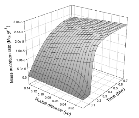
Figure 7: The mass accretion rate as a function of time and radial distance from the center of a pressure-free cloud that has initial radial gas density distribution $\rho=\rho_{\rm c}/[1+(r/r_{c})^{2}]$, in which $\rho_{\rm c}=7.5\times 10^{4}$ cm^-3 and $r_{\rm c}=0.033$ pc.

A.3.1 Modified isothermal sphere

First, we consider the radial gas density profile of a modified isothermal sphere: $\rho=\rho_{\rm c}/[1+(r/r_{c})^{2}]$ (Binney & Tremaine BT 1987), where $\rho_{\rm c}$ is the gas density in the center of a cloud and $r_{\rm c}$ is the radial scale length. Figure 7 shows $\dot{M}(r,t)$ of a pressure-free cloud with $\rho_{\rm c}=5.5\times 10^{4}$ cm^-3 and $r_{\rm c}=0.033$ pc. The mass accretion rate increases with time and appears to approach a constant value at later times $t>0.7$ Myr. Note that the temporal evolution of the mass accretion rate depends on the radial distance $r$: $\dot{M}$ approaches faster a constant value at smaller $r$. This behavior of $\dot{M}(r,t)$ is independent of the adopted values of $\rho_{\rm c}$ and $r_{\rm c}$.

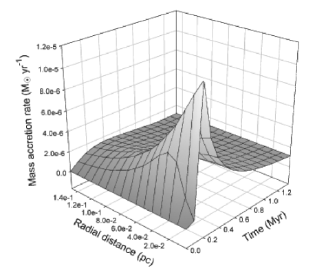
Figure 8: The same as Fig. 7 but for the initial gas density distribution $\rho=\rho_{\rm c}/[1+(r/r_{c})^{3}]$.

A.3.2 A steeper profile

The submillimeter and mid-infrared observations of Ward-Thompson et al. (WT 1999) and Bacmann et al. (Bacmann 2000) suggest that the gas density in the envelope of a starless core falls off steeper than $r^{-2}$. As a second example, we consider a pressure-free cloud with the initial gas density profile $\rho=\rho_{\rm c}/[1+(r/r_{\rm c})^{3}]$ and plot the corresponding mass accretion rate $\dot{M}(r,t)$ in Fig. 7. The values of $\rho_{\rm c}$ and $r_{\rm c}$ are retained from the previous example. As is seen, the temporal evolution of $\dot{M}$ strongly depends on the radial distance $r$. At $r\la 10^{4}$ AU, the mass accretion rate has a well-defined maximum at $t\approx 0.21$ Myr, when the central gas density has exceeded $10^{10}$ cm^-3 (the central stellar core formation). After stellar core formation, $\dot{M}$ drops as $\sim t^{-1}$. At $r>10^{4}$ AU, the temporal evolution of $\dot{M}$ does not show a well-defined maximum.

References

- 1 André, P., Motte, F., Bacmann, A., Belloche, A., 1999, in Nakamoto, T., ed., Star Formation 1999. Nobeyama Radio Observatory, Nobeyama, p. 145
- 2 André, P., Ward-Thompson, D., Barsony, M., 1993, 406, 122
- 3 André, P., Ward-Thompson, D., Barsony, M., 2000, in Mannings, V., Boss, A. P., Russell, eds., Protostars and Planets IV. Univ. Arizona Press, Tucson, p. 59
- 4 André, P., Motte, F., Belloche, A., 2001, in Montmerle, T., André, P., eds, ASP Conf. Ser. Vol. 243, From Darkness to Light. Astron.Soc.Pac., San Francisco, p. 209
- 5 Bacmann, A., André, P., Puget, J. L. et al., 2000, A&A, 314, 625
- 6 Basu, S., 1997, ApJ, 485, 240
- 7 Basu, S., Ciolek, G. E., 2004, ApJ, 607, L39
- 8 Basu, S., Mouschovias, T. Ch., 1994, ApJ, 432, 720
- 9 Basu, S., Mouschovias, T. Ch., 1995, ApJ, 453, 271
- 10 Binney, J., Tremaine, S., 1987, Galactic Dynamics. Princeton Univ. Press, Princeton
- 11 Bonnor, W. B., 1956, MNRAS, 116, 351
- 12 Bontemps, S., André, P., Terebey, S., Cabrit, S. 1996, A&A, 311, 858 (BATC)
- 13 Chandrasekhar, S., 1939, An Introduction to the Study of Stellar Structure. Univ. Chicago Press, Chicago
- 14 Ciolek, G. E., Mouschovias, T. Ch., 1993, ApJ, 418, 774
- 15 Ciolek, G. E., Königl, A., 1998, ApJ, 504, 257
- 16 Ebert, R., 1957, Afz, 42, 263
- 17 Foster, P. N., Chevalier, R. A., 1993, ApJ, 416, 303
- 18 Henriksen, R., André, P., Bontemps, S., 1997, A&A, 323, 549
- 19 Hunter, C., 1962, ApJ, 136, 594
- 20 Hunter, C., 1977, ApJ, 218, 834
- 21 Johnstone, D., Wilson, C. D., Moriarty-Schieven, G. et al., 2000, ApJ, 545, 327
- 22 Kenyon, S. J., Calvet, N., Hartmann, L. 1993, ApJ, 414, 676
- 23 Larson, R. B., 1969, MNRAS, 145, 271
- 24 Luhman, K. L., 2004, ApJ, 617, 1216
- 25 Masunaga, H., Inutsuka, S., 2000, ApJ, 531, 350
- 26 Moneti, A., Pipher, J. L., Helfer, H. L., McMillan, R. S., Perry, M. L., 1984, ApJ, 282, 508
- 27 Mönchmeyer, R., Müller, E., 1989, A&A, 217, 351
- 28 Motte, F., André, P., 2001, A&A, 365, 440
- 29 Ogino, S., Tomisaka, K., Nakamura, F., 1999, PASJ, 51, 637
- 30 Penston, M. V., 1969, MNRAS, 144, 425
- 31 Shu, F. H., 1977, ApJ, 214, 488
- 32 Shu, F. H., Adams, F. C., Lizano, S., 1987, ARA&A, 25, 23
- 33 Shu, F. H., Li, Z.-Y., Allen, A., 2004, ApJ, 601, 930
- 34 Stahler, S. W., 1988, ApJ, 332, 804
- 35 Stone, J. M., Norman, M. L., 1992, ApJS, 80, 753
- 36 Tomisaka, K., 1996, PASJ, 48, L97
- 37 Vorobyov, E. I., Tarafdar, S. P., 1999, A&ATr, 17, 407
- 38 Ward-Thompson, D., Motte, F., André, P., 1999, MNRAS, 305, 143
- 39 Whitworth, A. P., Summers, D., 1985, MNRAS, 214, 1
- 40 Whitworth, A. P., Ward-Thompson, D., 2001, ApJ, 547, 317
- 41 Winkler, K.-H. A., Newman, M. J., 1980, ApJ, 236, 201
- 42 Zuckerman, B., Evans, N. J., 1974, ApJ, 192, L149