A New Relation between GRB Rest-Frame Spectra and Energetics and Its Utility on Cosmology

Abstract

We investigate the well-measured spectral and energetic properties of 20 gamma-ray bursts (GRBs) in their cosmological rest frames. We find a tight relation between the isotropic-equivalent $\gamma$-ray energy $E_{\rm iso}$, the local peak energy $E^{\prime}_{p}$ of the $\nu F_{\nu}$ spectrum, and the local break time $t^{\prime}_{b}$ of the GRB afterglow light curve, which reads $E_{\rm iso}\,t^{\prime}_{b}\propto E^{\prime\,1.95\pm 0.08}_{p}$ ($\chi^{2}_{\nu}=1.40$; $\Omega_{M}=0.27$, $\Omega_{\Lambda}=0.73$). Such a power-law relation can be understood via the high-energy radiation processes for the GRB prompt emission accompanying the beaming effects. We then consider this relation as an intrinsic one for the observed GRB sample, and obtain a constraint on the mass density $\Omega_{M}=0.24^{+0.16}_{-0.12}$ ($1\sigma$) for a flat $\Lambda$CDM universe, and a $\chi^{2}_{\rm dof}=1.33$ for $\Omega_{M}\approx 0.3$ and $\Omega_{\Lambda}\approx 0.7$. Ongoing GRB observations in the Swift era are expected to confirm this relation and make its cosmological utility progress much.

1 Introduction

Gamma-ray bursts (GRBs) are the most powerful explosions in the universe since the Big Bang. Their cosmological origins are identified by the redshift measurements of their exploded remnants, usually named “GRB afterglows”, or their host galaxies. GRBs are common regarded as jetted phenomena, supported by the observational evidence that an achromatic break appears in the afterglow light curve, which declines more steeply than in the spherical model largely due to the edge effect and the laterally spreading effect (Rhoads 1999; Sari et al. 1999) or the off-axis viewing effect (Rossi, Lazzati & Rees 2002; Zhang & Mészáros 2002a; Berger et al. 2003). With the advantages of huge energy release for the prompt emission and immunity to dust extinction for the $\gamma$-ray photons, GRBs are widely believed to be detectable out to a very high redshift of $z\sim 10-20$ (Lamb & Reichart 2000; Ciardi & Loeb 2000; Bromm & Loeb 2002; Gou et al. 2004).

Similar to the Phillips relation in Type Ia supernovae (SNe Ia; Phillips 1993), a tight relation in GRBs, linking a couple of energetic and observational properties, could make GRBs new standard candles. Amati et al. (2002) reported a power-law relation between the isotropic-equivalent $\gamma$-ray energy $E_{\rm iso}$ of a GRB and its rest-frame $\nu F_{\nu}$ peak energy $E^{\prime}_{p}$. Unfortunately, the large scatter around this relation stymies its cosmological purpose. However, after joining the burst’s half-opening angle $\theta$, Ghirlanda et al. (2004a) found that a tight relation is instead between the collimation-corrected energy $E_{\gamma}$ and $E^{\prime}_{p}$, which reads $E_{\gamma}\equiv E_{\rm iso}(1-\cos\theta)\propto E^{\prime\,\kappa}_{p}$ ($\kappa$ is the power). Recently, Liang & Zhang (2005) reported a multi-variable relation between $E_{\rm iso}$, $E^{\prime}_{p}$, and the local achromatic break $t^{\prime}_{b}$ of the burst’s afterglow light curve, i.e., $E_{\rm iso}\propto E^{\prime\,\kappa_{1}}_{p}t^{\prime\,\kappa_{2}}_{b}$ ($\kappa_{1}$ and $\kappa_{2}$ are the powers). Applying these two relations to different observed GRB samples, meaningful cosmological constraints have been performed in a series of works (e.g. Dai, Liang & Xu 2004; Ghirlanda et al. 2004b; Firmani et al. 2005; Xu, Dai & Liang 2005; Ghisellini et al. 2005; Qin et al. 2005; Mortsell & Sollerman 2005; Liang & Zhang 2005; Bertolami & Silva 2005; Lamb et al. 2005 for a GRB mission plan to investigate the properties of dark energy).

In this paper we investigate the well-measured spectral and energetic properties of the up-to-date 20 GRBs in their cosmological frames and report a new relation between $E_{X}$ ($E_{X}\equiv E_{\rm iso}\,t^{\prime}_{b}$) and $E^{\prime}_{p}$, which is $E_{X}\propto E^{\prime\,b}_{p}$ (where $b$ is the power). More importantly, inspiring constraints on cosmological parameters can be achieved if this newly found relation is indeed an intrinsic one for the observed GRB sample.

2 Data Analysis and Statistical Result

The “bolometric” isotropic-equivalent energy of a GRB is given by

$$E_{\rm iso}=4\pi d_{L}^{2}S_{\gamma}k(1+z)^{-1},$$ (1)

where $S_{\gamma}$ is the fluence in the observed bandpass and $k$ is a multiplicative correction relating the observed bandpass with a standard rest-frame bandpass (1-$10^{4}$ keV) (Bloom, Frail & Sari 2001), with its fractional uncertainty

$$\left({\frac{{\sigma_{E_{\rm iso}}}}{{E_{\rm iso}}}}\right)^{2}=\left({\frac{{\sigma_{S_{\gamma}}}}{{S_{\gamma}}}}\right)^{2}+\left({\frac{{\sigma_{k}}}{k}}\right)^{2}.$$ (2)

Thus, the collimation-related energy $E_{X}$ (see $\S 4$ of this work) is

$$E_{X}\equiv E_{\rm iso}\,t^{\prime}_{b}=4\pi d_{L}^{2}S_{\gamma}k\,t_{b}(1+z)^{-2},$$ (3)

where $t_{b}$ is the observed break time of the afterglow light curve in the optical band, with its fractional uncertainty

$$\left({\frac{{\sigma_{E_{X}}}}{{E_{X}}}}\right)^{2}=\left({\frac{{\sigma_{S_{\gamma}}}}{{S_{\gamma}}}}\right)^{2}+\left({\frac{{\sigma_{k}}}{k}}\right)^{2}+\left({\frac{{\sigma_{t_{b}}}}{{t_{b}}}}\right)^{2}.$$ (4)

To calculate $k$-correction of a burst, one is required to know its spectral parameters fitted by the Band function, i.e., the low-energy spectral index $\alpha$, the high-energy spectral index $\beta$, and the observed peak energy $E_{p}\equiv E^{\prime}_{p}/(1+z)$ (Band et al. 1993). In this paper, we considered those GRBs with known redshifts, fluences, spectral parameters, and break times, and thus collected a sample of 20 bursts shown in Table 1. The criterions of our data selection are: (1) The fluence and spectral parameters of a burst are chosen from the same original literature as possible. If different fluences are reported in that literature, we choose the measurement in the widest energy band. If this criterion is unsatisfied, we choose the fluence measured in the widest energy band available in other literature; (2) The observed break time for each burst is taken from its data in the optical band; (3) When the fractional uncertainties of $E_{p}$, $S_{\gamma}$ and $k$ are not reported in the literature, they are taken to be $20\%$, $10\%$ and $5\%$, respectively; (4) To be more reliable, a lower limit of the fractional uncertainty of $t_{b}$ is set to be $10\%$.

In this section, we investigate the $E_{\rm iso}-E^{\prime}_{p}$ and $E_{X}-E^{\prime}_{p}$ relations for a Friedmann-Roberston-Walker cosmology with mass density $\Omega_{M}$ and vacuum energy density $\Omega_{\Lambda}$. Therefore, the theoretical luminosity distance in equations (1) and (3) is given by

$$d_{L} = c(1+z)H_{0}^{-1}|\Omega_{k}|^{-1/2}{\rm sinn}\{|\Omega_{k}|^{1/2}$$ (5)

$$\times\int_{0}^{z}dz[(1+z)^{2}(1+\Omega_{M}z)-z(2+z)\Omega_{\Lambda}]^{-1/2}\},$$

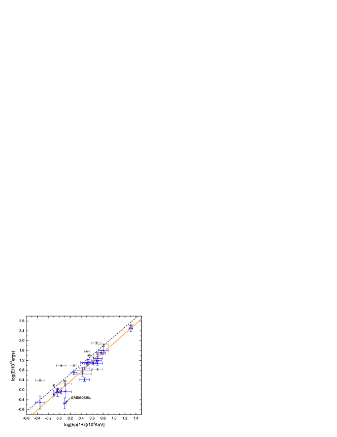
Figure 1: The $E_{X}/E_{\rm iso}-E^{\prime}_{p}$ plane. Circles represent $E_{X}$ vs. $E^{\prime}_{p}$ for 20 GRBs, while squares denote $E_{\rm iso}$ vs. $E^{\prime}_{p}$. Solid and dashed lines are the best fits of the $E_{X}-E^{\prime}_{p}$ and $E_{\rm iso}-E^{\prime}_{p}$ relations, using $\Omega_{M}=0.27$, $\Omega_{\Lambda}=0.73$, and $h=0.71$.

where $\Omega_{k}=1-\Omega_{M}-\Omega_{\Lambda}$, $H_{0}\equiv 100\,h\,\,{\rm{km\,s^{-1}Mpc^{-1}}}$ is the present Hubble constant, and “sinn” is $\sinh$ for $\Omega_{k}>0$ and $\sin$ for $\Omega_{k}<0$. For $\Omega_{k}=0$, equation (5) degenerates to be $c(1+z)H_{0}^{-1}$ times the integral (Carroll et al. 1992). According to the conclusions of the Wilkinson Microwave Anisotropy Probe (WMAP) observations, we here choose $\Omega_{M}=0.27$, $\Omega_{\Lambda}=0.73$, and $h=0.71$ (e.g. Spergel et al. 2003). The dashed and solid lines in Figure 1 respectively represent the best-fit powerlaws for the $E_{\rm iso}-E^{\prime}_{p}$ and $E_{X}-E^{\prime}_{p}$ relations (weighting for the uncertainties on both coordinates, see Press et al. 1999). We find

$$\frac{{E_{{\rm{iso}}}}}{{10^{52}\,{\rm{ergs}}}}=10^{0.27\pm 0.03}\left({\frac{{E^{\prime}_{p}}}{{10^{2}\,{\rm{KeV}}}}}\right)^{1.90\pm 0.06}$$ (6)

with a reduced $\chi^{2}=5.99$, and

$$\frac{{E_{X}}}{{10^{52}\,{\rm{ergs}}}}=10^{-0.04\pm 0.04}\left({\frac{{E^{\prime}_{p}}}{{10^{2}\,{\rm{KeV}}}}}\right)^{1.95\pm 0.08}$$ (7)

with a reduced $\chi^{2}=1.40$. As can be seen, although the power of the $E_{\rm iso}-E^{\prime}_{p}$ relation in this work is roughly consistent with that in Amati et al. (2002) derived from 9 BeppoSAX bursts, i.e., $E^{\prime}_{p}\propto E^{\,0.52\pm 0.06}_{\rm iso}$ ($\chi^{2}_{\nu}=0.91$), the dispersion around this relation increases seriously. Instead, the scatter of the $E_{X}-E^{\prime}_{p}$ relation is rather small. One may notice that it is the $E_{X}-E^{\prime}_{p}$ relation rather than the Amati relation whose power more converges at $\sim 2$. Based on the above statistical findings, we consider the $E_{X}-E^{\prime}_{p}$ relation for the observed GRB sample to constrain cosmological parameters.

3 Constraints on Cosmological Parameters

The $E_{X}-E^{\prime}_{p}$ relation can be given by

$$E_{X}/10^{52}{\rm{ergs=}}10^{a}(E^{\prime}_{p}/100{\rm{KeV}})^{b},$$ (8)

where the dimensionless parameters $a$ and $b$ are assumed to have no covariance. Combining equations (3) and (8), we derive the apparent luminosity distance as

$$d_{L}=9.142\times 10^{a/2}(E^{\prime}_{p}/100)^{b/2}(1+z)(kS_{\gamma}t_{b})^{-1/2}{\rm{Mpc}},$$ (9)

with its fractional uncertainty being

$$\left({\frac{{\sigma_{d_{L}}}}{{d_{L}}}}\right)^{2} = \left({\frac{{\sigma_{S_{\gamma}}}}{{2S_{\gamma}}}}\right)^{2}+\left({\frac{{\sigma_{k}}}{{2k}}}\right)^{2}+\left({\frac{{\sigma_{t_{b}}}}{{2t_{b}}}}\right)^{2}+\left({\frac{b}{2}\frac{{\sigma_{E_{p}}}}{{E_{p}}}}\right)^{2}$$ (10)

$$+\left({\frac{{\ln 10}}{2}\sigma_{a}}\right)^{2}+\left({\frac{{\ln(E^{\prime}_{p}/10^{2})}}{2}\sigma_{b}}\right)^{2},$$

where all the quantities are assumed to be independent of each other and their uncertainties follow Gaussian distributions. The distance modulus is calculated by $\mu=5\log(d_{L}/{\rm{Mpc}})+25$, and its uncertainty is computed through $\sigma_{\mu}=(5/\ln 10)(\sigma_{d_{L}}/d_{L})$.

Although the $E_{X}-E^{\prime}_{p}$ relation is similar to the Phillips relation in SNe Ia, the methods by which to constrain cosmological parameters are different (Riess et al. 1998; Firmani et al. 2005, Xu et al. 2005). For SNe Ia, a Phillips-like relation is known to those relatively high-$z$ objects after it has been calibrated by nearby well-observed SNe Ia, because the theoretical luminosity distance is irrelevant with cosmological parameters, i.e. $d_{L}=z(c/H_{0})$, when $z\ll 1$. While for GRBs, one won’t know that sole set of $(a,b)$- parameters in the $E_{X}-E^{\prime}_{p}$ relation until a low-$z$ GRB sample is established. Therefore, the $\chi^{2}$ statistic for GRBs is

$$\chi^{2}(\Omega,a,b|h)=\sum\limits^{20}_{k=1}{\left[{\frac{{\mu_{{\rm{th}}}(z_{k};\Omega|h)-\mu_{{\rm{obs}}}(z_{k};\Omega,a,b|h)}}{{\sigma_{\mu_{{\rm{obs}}}(z_{k};\,\Omega,\,a,\,b,\,\sigma_{a}/a,\,\sigma_{b}/b)}}}}\right]}^{2},$$ (11)

where $\Omega\equiv(\Omega_{M},\,\Omega_{\Lambda})$ denotes a certain cosmology, and $h$ is taken as 0.71 in this work.

We carry out a Bayesian approach to obtain GRBs’ constraints on cosmological parameters. For clarity, we divide it into three stages with the detailed steps as follows:

Stage I

(1) fix $\Omega_{i}\equiv(\Omega_{M},\Omega_{\Lambda})_{i}$, (2) calculate $\mu_{\rm th}$ and $E_{X}$ for each burst for that cosmology, (3) best fit the $E_{X}-E^{\prime}_{p}$ relation to yield $(a,b)_{i}$ and $(\sigma_{a}/a,\ \sigma_{b}/b)_{i}$, (4) apply the best-fit relation parametrized by $(a,b)_{i}$ and $(\sigma_{a}/a,\ \sigma_{b}/b)_{i}$ to the observed sample, and thus derive $\mu_{\rm obs}$ and $\sigma_{\mu_{\rm obs}}$ for each burst for that cosmology, (5) repeat Steps 1$-$4 from $i=1$ to $i={\rm N}$ to obtain $\mu_{\rm th}$, $\mu_{\rm obs}$ and $\sigma_{\mu_{\rm obs}}$ for each burst for each cosmology;

Stage II

(6) re-fix $\Omega_{j}$, (7) calculate $\chi^{2}(\Omega_{j}|\Omega_{i})$ by comparing $\mu_{\rm th}(\Omega_{j})$ with $\mu_{\rm obs}(\Omega_{i})$, $\sigma_{\mu_{\rm obs}}(\Omega_{i})$, and then convert it to a conditional probability, i.e., probability for $\Omega_{j}$ which is contributed by the relation calibrated for $\Omega_{i}$, by the formula of $P(\Omega_{j}|\Omega_{i})\propto\exp[-\chi^{2}(\Omega_{j}|\Omega_{i})/2]$, (8) repeat Step 7 from $i=1$ to $i=\rm N$ to obtain an iterative probability for cosmology $\Omega_{j}$ by $P^{\rm ite}(\Omega_{j})\propto\sum\limits_{i}{\exp[-\chi^{2}(\Omega_{j}|\Omega_{i})/2]\times P^{\rm ini}(\Omega_{i})}$ (here the initial probability for each cosmology is regarded as equal, i.e., $P^{\rm ini}(\Omega)\equiv 1$), (9) repeat Steps 6$-$8 from $j=1$ to $j=\rm N$ to obtain an iterative probability $P^{\rm ite}(\Omega)$ for each cosmology;

Stage III

The iterative probability $P^{\rm ite}(\Omega)$ for each cosmology derived on Step 9 is no longer equal to its initial probability $P^{\rm ini}(\Omega)$, but it has not reached the final/converged probability $P^{\rm fin}(\Omega)$. So the following process is to (10) assign $P^{\rm ite}(\Omega)$ on Step 9 to $P^{\rm ini}(\Omega)$ on Step 8, then repeat Steps 8$-$9, and thus reach another set of iterative probabilities for each cosmology, (11) run the above iteration cycle again and again until the probability for each cosmology converges, i.e., $P^{\rm ite}(\Omega)\Rightarrow P^{\rm fin}(\Omega)$ after tens of cycles.

In this method, to calculate the probability for a favored cosmology, we consider contributions of all the possible $E_{X}-E^{\prime}_{p}$ relations associated with their weights. The conditional probability $P(\Omega_{j}|\Omega_{i})$ denotes the contribution of some certain relation, and $P^{\rm fin}(\Omega_{i})$ weights the likelihood of this relation for its corresponding cosmology. Therefore, this Bayesian approach can be formulized by

$$P^{\rm fin}(\Omega_{j})={{\sum\limits_{i=1}^{\rm{N}}{P{\rm{(}}\Omega_{j}{\rm{|}}\Omega_{i}{\rm{)}}\times P^{\rm fin}{\rm{(}}\Omega_{i}{\rm{)}}}}\mathord{\left/{\vphantom{{\sum\limits_{i=1}^{\rm{N}}{P{\rm{(}}\Omega_{j}{\rm{|}}\Omega_{i}{\rm{)}}\times P_{\rm GRB}{\rm{(}}\Omega_{i}{\rm{)}}}}{\sum\limits_{i=1}^{\rm{N}}{P^{{\rm{fin}}}{\rm{(}}\Omega_{i}{\rm{)}}}}}}\right.\kern-1.2pt}{\sum\limits_{i=1}^{\rm{N}}{P^{\rm fin}{\rm{(}}\Omega_{i}{\rm{)}}}}}\,\,\,\,\,\,(j=1,{\rm N}).$$

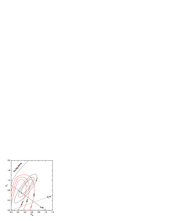
Figure 2: Joint confidence intervals (68.3%, 90%, 99%) in the $\Omega_{M}-\Omega_{\Lambda}$ plane from 20 observed GRBs (solid contours), and from 157 gold SNe Ia (dashed contours). Red and black crosses mark the best fits of the two samples, while black dot denotes the concordance model of $\Omega_{M}=0.3$.

Shown in Figure 2 are the constraints for $(\Omega_{M},\Omega_{\Lambda})$ from 20 observed GRBs (solid contours), using the likelihood procedure presented here. The GRB dataset is consistent with $\Omega_{M}\approx 0.3$ and $\Omega_{\Lambda}\approx 0.7$, yielding a $\chi^{2}_{\rm dof}=1.33$. For a flat universe, we measure $\Omega_{M}=0.24^{+0.16}_{-0.12}$ at the $68.3\%$ confidence level (C.L.). The best-fit point is $\Omega_{M}=0.24$ and $\Omega_{\Lambda}=0.76$ (red cross). Shape of the elliptic confidence contours trends to well constrain $\Omega_{M}$ and provide evidence for cosmic acceleration with an enlarged GRB sample. For comparison, we also plot the constraints from 157 gold SNe Ia in Riess et al. (2004) (dashed contours). Closed $\Omega_{M}-\Omega_{\Lambda}$ ranges derived from these two datasets at the same C.L.s have conveyed the advantages of high-$z$ distance indicators in constraining cosmological parameters as well as other cosmological issues. Additionally, GRBs are complementary to SNe Ia on the cosmological aspect. We see from the figure that a combination of SNe and GRBs wound make the cosmic model of $\Omega_{M}\approx 0.3$ and $\Omega_{\Lambda}\approx 0.7$ more favored, thus better in agreement with the result form WMAP observations (e.g. Bennett et al. 2003). GRBs are hopeful to be new standard candles.

4 Conclusions and Discussion

We report a new relation between GRB rest-frame energetics and spectra, which is $E_{\rm iso}\,t^{\prime}_{b}/10^{52}{\rm{ergs}}=10^{-0.04\pm 0.04}(E^{\prime}_{p}/100{\rm{KeV}})^{1.95\pm 0.08}$ ($\chi^{2}_{\nu}=1.40$) for $\Omega_{M}=0.27$, $\Omega_{\Lambda}=0.73$ and $h=0.71$. Considering this power-law relation for the 20 observed GRBs, we find a constraint on the mass density $\Omega_{M}=0.24^{+0.16}_{-0.12}$ ($1\sigma$) for a flat universe together with a $\chi^{2}_{\rm dof}=1.33$ for $\Omega_{M}\approx 0.3$ and $\Omega_{\Lambda}\approx 0.7$.

As previously discussed, the Ghirlanda relation reads $E_{\gamma}\equiv E_{\rm iso}(1-\cos\theta)\propto E^{\prime\,\kappa}_{p}$ ($\kappa$ is the power) under the framework of uniform jet model. Within this model, one can calculate the half-opening angle of a GRB jet by $\theta\propto t^{\prime\,3/8}_{b}(n\eta_{\gamma})^{1/8}E_{{\rm{iso}}}^{-1/8}$, where $n$ is the uniform circumburst medium density, and $\eta_{\gamma}$ denotes the conversion efficiency of the initial ejecta’s kinetic energy to $\gamma$-ray energy release (Rhoads 1999; Sari et al. 1999). Thanks to strong collimation for GRBs, i.e. $\theta\ll 1$, the Ghirlanda relation becomes $E_{\gamma}\propto(E_{{\rm{iso}}}\,t^{\prime}_{b})^{3/4}(n\eta_{\gamma})^{1/4}$. In Ghirlanda et al. (2004a), the term of $n\eta_{\gamma}$ was assumed to be highly clustered for the whole sample of 15 bursts presented there, thus the Ghirlanda relation turns out to be $E_{\gamma}\propto(E_{{\rm{iso}}}\,t^{\prime}_{b})^{3/4}$. So if $E_{{\rm{iso}}}\,t^{\prime}_{b}\propto E^{\prime\,b}_{p}$ ($b\sim 2$), there will be $E_{\gamma}\propto E^{\prime\,\kappa}_{p}$ ($\kappa\sim 1.5$). In this sense, the $E_{\gamma}-E^{\prime}_{p}$ and $E_{X}-E^{\prime}_{p}$ relations are consistent with each other. However, $\eta_{\gamma}$ should be different from burst to burst (e.g. $\leq 1\%-90\%$), and $n$ is variable for a burst in the wind environment and may expand in several orders (see Friedman & Bloom 2004 and references therein). Additionally, these two observables and their uncertainties are very difficult to be reliably estimated. Therefore, if the Ghirlanda relation is used to measure cosmology, the resulting constraints would depend on different input assumptions of $\eta_{\gamma}$ and $n$. For contrast, such difficulties have been circumvented when applying the $E_{X}-E^{\prime}_{p}$ relation. Moreover, Liang & Zhang (2005) reported a generalized relation between GRB rest-frame spectra and energetics could be written as $E_{{\rm{iso}}}/10^{52}\,{\rm{ergs}}=({0.85\pm 0.21})\times{(E^{\prime}_{p}/{\rm 100\,KeV})}^{1.94\pm 0.17}\times(t^{\prime}_{b}/1\,{\rm{day}})^{-1.24\pm 0.23}$ for a flat universe of $\Omega_{M}=0.28$, using a multiple variable regression method for the 15 bursts presented there. Their conclusion is consistent with our statistical result (see $\S 2$ in this work). More loose constraints, however, were performed when the uncertainties of the fitted parameters in this relation were included into the error of the apparent distance modulus (see Fig 11 in Liang & Zhang 2005). Among the discussed three relations, the $E_{X}-E^{\prime}_{p}$ relation is the simplest and the latter two have the advantage of making the relations explicitly model-independent and eliminating the needs to marginalize over the unknown $\eta_{\gamma}$ and $n$.

So what is the underlying theoretical basis for the $E_{X}-E^{\prime}_{p}$ relation? At the present stage, plausible explanations mainly include: the standard synchrotron mechanisms in relativistic shocks (e.g. Zhang & Mészáros 2002b; Dai & Lu 2002), the high-energy emission form off-axis relativistic jets (e.g. Yamazaki et al. 2004; Eichler & Levinson 2004; Levinson & Eichler 2005), and the dissipative photosphere model producing a relativistic outflow (e.g. Rees & Mészáros 2005). The scaling relation depends on the details of each model, and it resembles the observational result under certain simplification. Although models are different, the relation they support has made GRBs towards more and more standardized candles.

Table 1:

Sample of 20 $\gamma$-ray bursts

GRB	Redshift	$E_{p}(\sigma_{E_{p}})\tablenotemark{a}$	$[\alpha,\beta]\tablenotemark{a}$	$S_{\gamma}(\sigma_{S_{\gamma}})\tablenotemark{b}$	${\rm Bandpass}\tablenotemark{b}$	$t_{\rm b}(\sigma_{t_{\rm b}})\tablenotemark{c}$	${\rm References}\tablenotemark{d}$
		KeV		$10^{-6}\,{\rm erg\,cm^{-2}}$	KeV	day	($E_{p}$, $S_{\gamma}$, $t_{\rm b}$)
970828…	0.9578	297.7[59.5]	-0.70, -2.07	96.0[9.6]	20-2000	2.2(0.4)	1,2,3
980703…	0.966	254.0[50.8]	-1.31, -2.40	22.6[2.26]	20-2000	3.4(0.5)	1,2,4
990123…	1.600	780.8(61.9)	-0.89, -2.45	300.0(40.0)	40-700	2.04(0.46)	5,5,6
990510…	1.619	161.5(16.0)	-1.23, -2.70	19.0(2.0)	40-700	1.57(0.16)	5,5,7
990705…	0.8424	188.8(15.2)	-1.05, -2.20	75.0(8.0)	40-700	1.0(0.2)	5,5,8
990712…	0.4331	65.0(10.5)	-1.88, -2.48	6.5(0.3)	40-700	1.6(0.2)	5,5,9
991216…	1.020	317.3[63.4]	-1.23, -2.18	194.0[19.4]	20-2000	1.2(0.4)	1,2,10
011211…	2.140	59.2(7.6)	-0.84, -2.30	5.0[0.5]	40-700	1.56(0.16)	11,2,12
020124…	3.200	120.0(22.6)	-1.10, -2.30	6.8[0.68]	30-400	3.0(0.4)	13,13,14
020405…	0.690	192.5(53.8)	0.00, -1.87	74.0(0.7)	15-2000	1.67(0.52)	15,15,15
020813…	1.255	212.0(42.0)	-1.05, -2.30	102.0[10.2]	30-400	0.43(0.06)	13,13,16
021004…	2.332	79.8(30.0)	-1.01, -2.30	2.55(0.60)	2 -400	4.74(0.47)	17,17,18
021211…	1.006	46.8(5.5)	-0.805,-2.37	2.17(0.15)	30-400	1.4(0.5)	19,19,20
030226…	1.986	97.1(20.0)	-0.89, -2.30	5.61(0.65)	2 -400	1.04(0.12)	17,17,21
030328…	1.520	126.3(13.5)	-1.14, -2.09	36.95(1.40)	2 -400	0.8(0.1)	17,17,22
030329…	0.1685	67.9(2.2)	-1.26, -2.28	110.0(10.0)	30-400	0.48(0.05)	23,23,24
030429…	2.658	35.0(9.0)	-1.12, -2.30	0.854(0.14)	2 -400	1.77(1.0)	17,17,25
041006…	0.7160	63.4[12.7]	-1.37, -2.30	19.9[1.99]	25-100	0.16(0.04)	26,26,27
050408…	1.2357	19.93(4.0)	-1.979,-2.30	1.90[0.19]	30-400	0.28(0.17)	28,28,29
050525a.	0.606	78.8(4.0)	-0.987,-8.839	20.1(0.50)	15-350	0.20(0.10)	30,30,30

References

- (1) Amati, L. et al. 2002, A&A, 390, 81
- (2) Amati, L. 2003, ChJAA, 3, 455
- (3) Andersen, M. I. et al. 2003, GCN, 1993
- (4) Band, D., Matteson, J., Ford, L., et al. 1993, ApJ, 413, 281
- (5) Barth, A. J. et al. 2003, ApJ, 584, L47
- (6) Barraud, C. et al. 2003, A&A, 400, 1021
- (7) Bennett, C. L. et al. 2003, ApJS, 148, 1
- (8) Berger, E. et al. 2002, ApJ, 581, 981
- (9) Berger, E. et al. 2003, Nature, 426, 154
- (10) Bertolami O. & Silva P. T. 2005, preprint, astro-ph/0507192
- (11) Björnsson, G. et al. 2001, ApJ, 552, L121
- (12) Bloom, J. S., Frail, D. A., & Sari, R. 2001, AJ, 121, 2879
- (13) Bloom, J. S., Frail, D. A., & Kulkarni, S. R. 2003, ApJ, 594, 674
- (14) Blustin, A. J., Band, D., Barthelmy, S. et al. 2005, preprint, astro-ph/0507515
- (15) Bromm, V., & Loeb, A. 2002, ApJ, 575, 111
- (16) Butler N., Vanderspek, R., Marshall, H. L. et al. 2004, GCN, 2808, see also http://space.mit.edu/HETE/Bursts/GRB041006
- (17) Carroll, S. M., Press, W. H., & Turner, E. L. 1992, ARA&A, 30, 499
- (18) Ciardi, B., & Loeb, A. 2000, ApJ, 540, 687
- (19) Crew, G. B. et al. 2003, ApJ, 599, 387
- (20) Dai, Z. G., & Lu, T. 2002, ApJ, 580, 1013
- (21) Dai, Z. G., Liang, E. W. & Xu, D. 2004, ApJ, 612, L101
- (22) Djorgovski, S. G. et al. 2001, ApJ, 562, 654
- (23) Eichler, D., & Levinson, A. 2004, ApJ, 614, L13
- (24) Firmani, C. et al. 2005, MNRAS, 360, 1
- (25) Frail, D. A. et al. 2003, ApJ, 590, 992
- (26) Friedman, A. S. & Bloom, J. S. 2005, ApJ, 627, 1
- (27) Ghirlanda, G., Ghisellini, G., & Lazzati, D. 2004a, ApJ, 616, 331
- (28) Ghirlanda, G., Ghisellini, G., Lazzati, D. & Firmani, C. 2004b, ApJ, 613, L13
- (29) Ghisellini G., Ghirlanda G., Firmani C., Avila-Reese V., 2005, preprint, astro-ph/0504306, review at the 4th Workshop Gamma-Ray Bursts in the Afterglow Era
- (30) Godet, O. et al. 2005, GCN, 3222
- (31) Gou, L. J., Mészáros, P., Abel, T. & Zhang, B. 2004, ApJ, 604, 508
- (32) Halpern, J. P., et al. 2000, ApJ, 543, 697
- (33) Holland, et al. 2003, AJ, 125, 2291
- (34) Holland, et al. 2004, AJ, 128, 1955
- (35) Jakobsson, P. et al. 2003, A&A, 408, 941
- (36) Jakobsson, P. et al. 2004, A&A, 427, 785
- (37) Jimenez, R., Band, D. L., & Piran, T., 2001, ApJ, 561, 171
- (38) Klose, S. et al. 2004, AJ, 128, 1942
- (39) Kulkarni, S. R. et al. 1999, Nature, 398, 389
- (40) Lamb, D. Q., & Reichart, D. E. 2000, ApJ, 536, 1
- (41) Lamb D. Q., Ricker G. R., Lazzati D., et al., 2005, astro-ph/0507362
- (42) Liang, E. W. & Zhang, B. 2005, ApJ in press (astro-ph/0504404)
- (43) Levinson, A. & Eichler, D. 2005, ApJL in press (astro-ph/0504125)
- (44) Masetti, N. et al. 2000, A&A, 354, 473
- (45) Mortsell E. & Sollerman J., 2005, JCAP, 0506, 009
- (46) Phillips, M. M. 1993, ApJ, 413, L105
- (47) Press, W. H. et al 1999, Numerical Recipes in Fortran, Cambridge University Press
- (48) Price, P. A. et al. 2003a, ApJ, 589, 838
- (49) Price, P. A. et al. 2003b, Nature, 423, 844
- (50) Qin Y. P., Zhang B. B., Dong Y. M. et al., 2005, preprint, astro-ph/0502373
- (51) Rees, M. J. & Mészáros, P. 2005, ApJ in press (astro-ph/0412702)
- (52) Rhoads, J. E. 1999, ApJ, 525, 737
- (53) Riess, A. G. et al. 1998, AJ, 116, 1009
- (54) Riess, A. G. et al. 2004, ApJ, 607, 665
- (55) Rossi, E., Lazzati, D. & Rees, M. J. 2002, MNRAS, 332, 945
- (56) Sakamoto, T. et al. 2004, preprint (astro-ph/0409128)
- (57) Sakamoto, T., Ricker, G., Atteia, J-L. et al. 2005, GCN, 3189, see also http://space.mit.edu/HETE/Bursts/GRB050408
- (58) Sari, R., Piran, T., & Halpern, J. P. 1999, ApJ, 519, L17
- (59) Spergel, D. N. et al. 2003, ApJS, 148, 175
- (60) Stanek, K. Z. et al. 1999, ApJ, 522, L39
- (61) Stanek, K. Z. et al. 2005, ApJ, 626, L5
- (62) Vanderspek, R. et al. 2004, AJ, 617, 1251
- (63) Xu, D., Dai, Z. G. & Liang, E. W. 2005, ApJ in press (astro-ph/0501458)
- (64) Yamazaki, R., Ioka, K., & Nakamura, T. 2004, ApJ, 606, L33
- (65) Zhang, B. & Mészáros, P. 2002a, ApJ, 571, 876
- (66) Zhang, B. & Mészáros, P. 2002b, ApJ, 581, 1236