Search templates for stochastic gravitational-wave backgrounds

Abstract

Several earth-based gravitational-wave (GW) detectors are actively pursuing the quest for placing observational constraints on models that predict the behavior of a variety of astrophysical and cosmological sources. These sources span a wide gamut, ranging from hydrodynamic instabilities in neutron stars (such as r-modes) to particle production in the early universe. Signals from a subset of these sources are expected to appear in these detectors as stochastic GW backgrounds (SGWBs). The detection of these backgrounds will help us in characterizing their sources. Accounting for such a background will also be required by some detectors, such as the proposed space-based detector LISA, so that they can detect other GW signals. Here, we formulate the problem of constructing a bank of search templates that discretely span the parameter space of a generic SGWB. We apply it to the specific case of a class of cosmological SGWBs, known as the broken power-law models. We derive how the template density varies in their three-dimensional parameter space and show that for the LIGO 4km detector pair, with LIGO-I sensitivities, about a few hundred templates will suffice to detect such a background while incurring a loss in signal-to-noise ratio of no more than 3%.

Multiple earth-based gravitational-wave (GW) detectors, including both resonant-mass and interferometric ones, are currently in operation aiming to make the first GW detection. As the sensitivities of these detectors improve, they will place interesting limits on astrophysical event rates and strengths of GW backgrounds, thus constraining or falsifying theoretical models. The subject of this paper is how to design a template bank for searching and bounding the strength of a stochastic GW background (SGWB). After formulating the problem for a general SGWB, of either astrophysical or cosmological origin, we apply it to the specific case of a SGWB with a spectral profile that belongs to a class predicted by a host of cosmological models, including inflationary and string-theoretic ones. This profile is known as the broken-power-law (BPL) spectrum, as described below Maggiore:1999vm ; Ungarelli:2003ty .

Searching for SGWBs with BPL-type spectra is important because some of the cosmological models that predict them also allow for their strengths to be large enough to be detectable in the near future. In particular, in the bandwidth of these detectors, their strengths can be several orders of magnitude higher than that predicted by the slow-roll inflationary model (SRIM) Maggiore:1999vm , while being consistent with extant observational constraints, such as arising from the anisotropy in the cosmic microwave background radiation Allen:1994xz ; Bose:2000 , the monitoring of radio pulses from several stable millisecond pulsars Kaspi:1994hp , and the empirical abundances of light elements in the universe kolbTurner90 . These models are, therefore, especially attractive to the detectors in operation. Additionally, GWs from those unresolved astrophysical sources that have a duty cycle appreciably larger than unity will appear as a stochastic signal in these detectors, some with BPL-type spectra and strengths that may be considerably larger than that of a cosmological SGWB predicted by SRIM Ferrari:1998jf . Indeed in the planned space-based detector LISA SysTech:2000rep , the background from unresolved galactic binaries is expected to be large enough to form a “source-confusion” noise and make it difficult to detect other GW signals Bender:1997hs . Although optimal statistics and templates for searching resolvable binaries exist Krolak:2004xp ; Rogan:2004wq , strategies for characterizing such a background in order to allow the detection of other sources are beginning to be explored. While we derive the limits on template spacings and template numbers for BPL-type cosmological spectra, the formalism given here for obtaining the search templates is general enough to be applicable to other cases, including astrophysical SGWBs.

We begin by briefly outlining the search statistic for a SGWB. The decision on whether a signal is present or absent in a detector output is often based on the examination of data that are noisy. In decision theory, the hypothesis that the data do not contain a signal is called the null hypothesis, $H_{0}$. Under the alternative hypothesis, $H_{1}$, the detector output is noise plus signal Helstrom . Thus, in the frequency domain, the output is

$$\tilde{h}(f;\mbox{\boldmath$\vartheta$})|_{H_{1}}=\tilde{n}(f)+{\cal A}\tilde{w}(f;\mbox{\boldmath$\vartheta$})\ \ ,$$ (1)

where $\tilde{n}(f)$ is the noise, ${\cal A}$ is the overall strength of the signal and $\tilde{w}(f;\mbox{\boldmath$\vartheta$})$ gives the spectral characteristics of the signal for different choices of the signal parameter vector, $\vartheta$. In general, the waveform will have the appearance:

$$\tilde{w}(f;\mbox{\boldmath$\vartheta$})=y(f;\mbox{\boldmath$\vartheta$})\exp\left[i\Psi(f;\mbox{\boldmath$\vartheta$})\right]\ \ ,$$ (2)

where $y(f;\mbox{\boldmath$\vartheta$})$ is a frequency-dependent amplitude, and $\Psi(f;\mbox{\boldmath$\vartheta$})$ is the signal phase. We assume that the detector noise has a zero-mean Gaussian probability distribution; it is described completely by the first two noise moments,

$$\overline{\tilde{n}(f)}=0\quad{\rm and}\quad\overline{\tilde{n}^{*}(f)\tilde{n}(f^{\prime})}=\frac{1}{2}P(|f|)\delta(f-f^{\prime})\ \ ,$$ (3)

where $P(|f|)$ is the one-sided noise power-spectral density (PSD) saulsonBook . We define the inner (or scalar) product of a pair of Fourier domain functions $\tilde{a}(f)$ and $\tilde{b}(f)$ as

$$\left(\tilde{a},\>\tilde{b}\right)=4\Re\int_{0}^{\infty}\!df\>\frac{\tilde{a}^{*}(f)\tilde{b}(f)}{m(f)}\ \ ,$$ (4)

where $\tilde{a}(f)$ and $\tilde{b}(f)$ are the Fourier transforms of temporal counterparts $a(t)$ and $b(t)$, respectively, and $m$ is an inverse weight that, typically, depends on the noise PSDs. Its exact form is decided by the detection statistic at hand.

The search templates are modeled after the waveform:

$$\tilde{u}(f;\mbox{\boldmath$\vartheta$}^{\prime})={\cal N}~{}\tilde{w}(f;\mbox{\boldmath$\vartheta$}^{\prime})\ \ ,$$ (5)

where $\mbox{\boldmath$\vartheta$}^{\prime}$ is the template parameter vector and ${\cal N}$ is a normalization factor. The inner-product of a template with itself,

$$\left(\tilde{u}(\mbox{\boldmath$\vartheta$}^{\prime}),\>\tilde{u}(\mbox{\boldmath$\vartheta$}^{\prime})\right)\equiv\kappa(\mbox{\boldmath$\vartheta$}^{\prime})\ \ ,$$ (6)

will be taken to be positive definite. Above, $\sqrt{\kappa}$ is the template norm, which is parameter dependent, in general. The normalization factor is related to the template norm as follows:

$${\cal N}(\mbox{\boldmath$\vartheta$}^{\prime})=\frac{\sqrt{\kappa(\mbox{\boldmath$\vartheta$}^{\prime})}}{2}\left[\int_{0}^{\infty}df\frac{y^{2}(f;\mbox{\boldmath$\vartheta$}^{\prime})}{m(f)}\right]^{-1/2}\,.$$ (7)

To test a hypothesis, one computes the cross-correlation of the data with the templates, viz., $\left(\tilde{h}(\mbox{\boldmath$\vartheta$})|_{H_{1}},\>\tilde{u}(\mbox{\boldmath$\vartheta$}^{\prime})\right)$, which is termed as the matched-filter output (MFO). Under $H_{1}$, the mean of the MFO is

$$\overline{S(\mbox{\boldmath$\vartheta$},\delta\mbox{\boldmath$\vartheta$})}:=\overline{\left(\tilde{h}(\mbox{\boldmath$\vartheta$})|_{H_{1}},\>\tilde{u}(\mbox{\boldmath$\vartheta$}^{\prime})\right)}\ \ ,$$ (8)

where $\delta\mbox{\boldmath$\vartheta$}\equiv\mbox{\boldmath$\vartheta$}-\mbox{\boldmath$\vartheta$}^{\prime}$.

One often uses in searches unit-norm templates, namely,

$$\kappa(\mbox{\boldmath$\vartheta$}^{\prime})=1\,.$$ (9)

The advantage of using such templates is that under $H_{1}$ and for $\delta\mbox{\boldmath$\vartheta$}=0$, the mean of the matched-filter output (MFO) is just the signal strength divided by the template normalization factor, i.e.,

$$\overline{S(\mbox{\boldmath$\vartheta$},\delta\mbox{\boldmath$\vartheta$}=0)}:=\overline{\left(\tilde{h}(\mbox{\boldmath$\vartheta$})|_{H_{1}},\>\tilde{u}(\mbox{\boldmath$\vartheta$})\right)}=\frac{\cal A}{{\cal N(\mbox{\boldmath$\vartheta$})}}\ \ ,$$ (10)

assuming that the signal model is perfect.

To quantify the effect of a mismatch, $\delta\mbox{\boldmath$\vartheta$}$, it is useful to introduce the match or ambiguity function:

$$M(\mbox{\boldmath$\vartheta$},\delta\mbox{\boldmath$\vartheta$}):=\left(\tilde{u}(\mbox{\boldmath$\vartheta$}),\>\tilde{u}(\mbox{\boldmath$\vartheta$}^{\prime})\right)\ \ ,$$ (11)

which tends to $\kappa(\mbox{\boldmath$\vartheta$})$ as $\delta\mbox{\boldmath$\vartheta$}\to 0$. Then the mean of the MFO can be shown from Eq. (8) to be

$$\overline{S(\mbox{\boldmath$\vartheta$},\delta\mbox{\boldmath$\vartheta$})}=\frac{\cal A}{{\cal N}(\mbox{\boldmath$\vartheta$})}M(\mbox{\boldmath$\vartheta$},\delta\mbox{\boldmath$\vartheta$})\,.$$ (12)

For small values of $\delta\mbox{\boldmath$\vartheta$}$, one can Taylor expand $M$ about $\delta\mbox{\boldmath$\vartheta$}=0$ to obtain

$$M(\mbox{\boldmath$\vartheta$},\delta\mbox{\boldmath$\vartheta$}) = \kappa\left(\mbox{\boldmath$\vartheta$}\right)\Big{[}1+d_{\mu}(\mbox{\boldmath$\vartheta$})\delta\vartheta^{\mu}$$ (13)

$$\quad\quad-g_{\mu\nu}(\mbox{\boldmath$\vartheta$})\delta\vartheta^{\mu}\delta\vartheta^{\nu}\Big{]}+{\cal O}\left(\delta\mbox{\boldmath$\vartheta$}^{3}\right)$$

where the Einstein summation convention over repeated indices, $\mu$ and $\nu$, was used and we defined

$$d_{\mu}:=\frac{1}{\kappa}\left[\frac{\partial M}{\partial\delta\vartheta^{\mu}}\right]_{\mbox{\boldmath$\delta\vartheta$=0}}\,,\>\>\>g_{\mu\nu}:=-\frac{1}{2\kappa}\left[\frac{\partial^{2}M}{\partial\delta\vartheta^{\mu}\partial\delta\vartheta^{\nu}}\right]_{\mbox{\boldmath$\delta\vartheta$=0}}\,.$$ (14)

Above, $g_{\mu\nu}$ can be interpreted as the metric on the parameter space that maps parameter mismatches into dips in the signal-to-noise ratio (SNR) Owen96 , provided $d_{\mu}$ vanishes. (The MFO of a unit-norm template is equivalent to the SNR boseCalib .)

It is important to note here that an observer also has the choice of using unnormalized templates, such that ${\cal N}=1$ in Eq. (5). This has the advantage that one does not have to recompute ${\cal N}$ and, therefore, the search templates, for every value of $\vartheta$ or every time $m$ (which can be the noise PSDs of the detectors) changes. Indeed, this choice was exercised by Ungarelli and Vecchio in their pioneering work in Ref. Ungarelli:2003ty . However, the disadvantage of such a choice is that the associated ambiguity function, $M(\mbox{\boldmath$\vartheta$},\delta\mbox{\boldmath$\vartheta$})$, has first order errors arising from parameter mismatches. Consequently, a “wrong” template (i.e., a template with $\delta\mbox{\boldmath$\vartheta$}\neq 0$) applied to a given data set can actually trigger an MFO that is larger than that of the “correct” template (with $\delta\mbox{\boldmath$\vartheta$}=0$) applied on the same data set. Use of constant-norm templates, such as the unit-norm ones defined above, avoids that problem.

To see explicitly why $d_{\mu}$ need not be zero for unnormalized templates, note that the associated ambiguity function obeys the Cauchy-Schwarz inequality dennery :

$$M(\mbox{\boldmath$\vartheta$},\delta\mbox{\boldmath$\vartheta$})=\left(\tilde{u}(\mbox{\boldmath$\vartheta$}),\>\tilde{u}(\mbox{\boldmath$\vartheta$}^{\prime})\right)\leq\sqrt{\kappa(\mbox{\boldmath$\vartheta$})\kappa(\mbox{\boldmath$\vartheta$}^{\prime})}\,.$$ (15)

Since, in general, $\kappa(\mbox{\boldmath$\vartheta$}^{\prime})$ can be larger than $\kappa(\mbox{\boldmath$\vartheta$})$ for some $\mbox{\boldmath$\vartheta$}^{\prime}\neq\mbox{\boldmath$\vartheta$}$, the rhs above can actually exceed $\kappa(\mbox{\boldmath$\vartheta$})$. Thus, $\kappa(\mbox{\boldmath$\vartheta$})$ need not be the maximum value of $M(\mbox{\boldmath$\vartheta$},\delta\mbox{\boldmath$\vartheta$})$ for unnormalized templates. Equation (13) then implies that $d_{\mu}$ need not be zero for such templates. However, for unit-norm templates the rhs of Eq. (15) is identically unity (and $\kappa(\mbox{\boldmath$\vartheta$})=1=\kappa(\mbox{\boldmath$\vartheta$}^{\prime})$), independent of the value of $\mbox{\boldmath$\vartheta$}^{\prime}$ or $\vartheta$. There, $M(\mbox{\boldmath$\vartheta$},\delta\mbox{\boldmath$\vartheta$})$ attains the maximum possible value of 1, when $\mbox{\boldmath$\vartheta$}^{\prime}=\mbox{\boldmath$\vartheta$}$. Thus, $d_{\mu}$ has to vanish for unit-norm (and constant-norm) templates, and $g_{\mu\nu}$ can assume its role as a parameter-space map.

Without any means for distinguishing a stochastic GW background in a detector from the detector’s intrinsic noise, the search for such a signal involves cross-correlating the outputs of a pair of detectors. As shown in Ref. Allen:1997ad , a useful statistic in decision making in this context is the cross-correlation (CC) statistic,

$$S:=\int_{-\infty}^{\infty}df\int_{-\infty}^{\infty}df^{\prime}\delta_{T}(f^{\prime}-f)\tilde{h}_{A}^{*}(f^{\prime})\tilde{h}_{B}(f)\tilde{u}(f)\ \ ,$$ (16)

where $\tilde{h}_{A}(f)$ is the inverse Fourier transform of the strain in the $A$th detector, $T$ is the observation time, $\delta_{T}(f)\equiv\int_{-T/2}^{T/2}dt~{}\exp(-i2\pi ft)$ is the finite-time approximation of the Dirac delta function, and $\tilde{u}(f)$ is a filtering function that will be determined below. The CC statistic can also be cast as the output of a matched filter:

$$S=\left(\tilde{K}|_{H_{1}},\>\tilde{u}\right)\ \ ,$$ (17)

where $\tilde{K}|_{H_{1}}$ is a functional of a pair of detector inputs:

$$\tilde{K}(f):=\frac{1}{2}\int_{-\infty}^{\infty}df^{\prime}\frac{\tilde{h}_{A}(f^{\prime})\tilde{h}_{B}^{*}(f)\delta_{T}(f^{\prime}-f)}{P_{A}(f)P_{B}(f)}$$ (18)

and the inner product is defined as in Eq. (4), with the inverse weight there set to $m=\left[P_{A}(f)P_{B}(f)\right]^{-1}$.

The product $\left[\tilde{h}_{A}^{*}(f^{\prime})\times\tilde{h}_{B}(f)\right]$ appearing in $S$ is a random variable since the SGWB strains, produced cosmologically or astrophysically (in some cases), are so. The detection statistic, therefore, is the mean of the CC statistic,

$$\overline{S}=\left(\overline{\tilde{K}|_{H_{1}}},\>\tilde{u}\right)\,.$$ (19)

And the variance of $S$ is

$$\sigma^{2}=\overline{S^{2}}-\left(\overline{S}\right)^{2}\ \ ,$$ (20)

which defines the noise-squared of $S$. If one assumes that the noise power in each detector due to terrestrial sources is much larger than that due to a SGWB, then Allen:1997ad

$$\sigma^{2} \approx \overline{S^{2}}\approx\frac{T}{4}\int_{-\infty}^{\infty}df~{}\left|\tilde{u}(f)\right|^{2}~{}P_{A}(|f|)P_{B}(|f|)$$ (21)

$$= \frac{T}{8}\left(\tilde{u},\>\tilde{u}\right)\,.$$

Above, it was assumed in the second approximation that the cross-correlation of the terrestrial noises in the two detectors is negligible. Thus, the SNR is

$${\rm SNR}=\frac{\overline{S}}{\sigma}=\sqrt{\frac{8}{T}}\frac{\left(\overline{\tilde{K}|_{H_{1}}},\>\tilde{u}\right)}{\sqrt{\left(\tilde{u},\>\tilde{u}\right)}}\ \ ,$$ (22)

which is maximized when the filtering function matches the signal, i.e.,

$$\tilde{u}=\lambda\overline{\tilde{K}|_{H_{1}}}\,.$$ (23)

where $\lambda$ is a proportionality constant. Although $\overline{S}$ and $\sigma$ are dependent on the choice of this constant, the SNR itself is independent of it.

Equation (23) suggests $\tilde{u}$ as templates for searching an astrophysical or cosmological SGWB, as long as the assumptions made above remain valid. We now concentrate in the rest of the paper on the search templates required for a cosmological SGWB. (A similar problem for the astrophysical SGWB will be studied elsewhere boseASGWB .) Theoretically, the strain due to a cosmological SGWB in each detector is expected to have a Gaussian probability distribution with zero mean; their variance-covariance matrix elements are given by Christensen:1992wi :

$$\overline{\tilde{h}_{A}^{*}(f)\Big{|}_{H_{1}}\tilde{h}_{B}(f^{\prime})\Big{|}_{H_{1}}} = \frac{3H_{0}^{2}}{20\pi^{2}}|f|^{-3}\gamma_{AB}(|f|)\Omega_{\rm GW}(|f|;\mbox{\boldmath$\vartheta$})$$ (24)

$$\times\delta(f-f^{\prime})\ \ ,$$

where $H_{0}$ is the Hubble constant, $\gamma_{AB}$ is the overlap-reduction function (ORF) for the detector pair Flanagan:1993ix , $\Omega_{\rm GW}$ is the energy density of the stochastic GW per logarithmic frequency bin divided by the critical energy density required to close the universe, and $\vartheta$ are the signal parameters on which it depends. Heretofore, we will identify $\gamma_{AB}\equiv\gamma$. The ORF for co-located and co-aligned interferometric detectors with orthogonal arms is normalized so that it is identically unity. Using the above strain-power density in the expression for $\overline{\tilde{K}|_{H_{1}}}$ yields the cosmological SGWB template:

$$\tilde{u}={\cal N}\frac{\gamma(|f|)\Omega_{\rm GW}(|f|;\mbox{\boldmath$\vartheta$})}{|f|^{3}P_{A}(|f|)P_{B}(|f|)}\ \ ,$$ (25)

where, for unit-norm templates,

$${\cal N}=\left[2\int_{-\infty}^{\infty}df\frac{\gamma^{2}(|f|)\Omega_{\rm GW}^{2}(|f|;\mbox{\boldmath$\vartheta$})}{f^{6}P_{A}(|f|)P_{B}(|f|)}\right]^{-1/2}\,.$$ (26)

We now show how to obtain the spacing between such templates on the $\vartheta$ parameter space such that its discreteness, $\delta\mbox{\boldmath$\vartheta$}$, is small enough to guarantee an SNR of $\geq$97% of that obtained in the ideal case of $\delta\mbox{\boldmath$\vartheta$}=0$,

.0.1 Single power-laws

Before studying the template spacings of the BPL spectra, let us consider the simpler case where $\Omega_{\rm GW}(f)$ is in the form of a single power-law (SPL) in frequency,

$$\Omega_{\rm GW}(f)=\Omega_{0}\left(\frac{f}{f_{p}}\right)^{k}\ \ ,$$ (27)

where $k$ is a real power, and $\Omega_{0}$ and $f_{p}$ are positive-definite real constants. In the bandwidths of LISA or LIGO-type detectors, the SGWB spectrum predicted by SRIM will appear as a special case of the above, with $k\approx 0$. In such a case the only intrinsic search parameter is the index $k$ and the ambiguity function can be expanded around $\delta k:=k-k^{\prime}=0$ as

$$M(k,\delta k)=1-\frac{1}{2}\left[\alpha(2)-\alpha^{2}(1)\right]\delta k^{2}+{\cal O}\left(\delta k^{3}\right)\ \ ,$$ (28)

where $\alpha\left(n\right)$ is the template-space mean of $\ln\left(f/f_{p}\right)$:

$$\alpha\left(n\right) = \left(\tilde{u}(k),\>\left[\ln\left(f/f_{p}\right)\right]^{n}\tilde{u}(k)\right)$$ (29)

$$= \int_{f_{-}/f_{p}}^{f_{+}/f_{p}}dx\frac{\gamma^{2}(f_{p}x)x^{2k-6}\left[\ln x\right]^{n}}{P_{A}(f_{p}x)P_{B}(f_{p}x)}$$

$$\times\left[\int_{f_{-}/f_{p}}^{f_{+}/f_{p}}dx\frac{\gamma^{2}(f_{p}x)x^{2k-6}}{P_{A}(f_{p}x)P_{B}(f_{p}x)}\right]^{-1}\,.$$

Above, $n$ is any real number, and $f_{-}$, $f_{+}$ are the lower and upper limits of the frequency integral, respectively. For the LIGO-Hanford (LHO) and -Livingston (LLO) pair, with LIGO-I sensitivity, we choose $f_{-}=40$Hz (determined by the detectors’ seismic-noise cut-off) and $f_{+}=512$Hz, respectively. For this inter-site correlation, the statistic does not receive any appreciable contribution from higher frequencies owing to a weak $\gamma(f)$. By contrast, for co-located interferometers, $\gamma(f)=1$ for all frequencies, and the upper cut-off frequency is determined by the worsening sensitivity due to the photon shot-noise lazzariniWeiss ; saulsonBook . An optimal way of computing the CC statistic on the data from a set of multiple detectors that includes a co-located pair, while accounting for intra-site terrestrial noise, was obtained in Ref. Lazzarini:2004hk . For searches in this kind of a detector network, the value of $f_{+}$ should be revised upward of 512Hz. As such, the expressions here are applicable to any pair of GW detectors. However, the template-spacings, number of templates, and the figures are computed for the LLO-LHO (4km) pair, with LIGO-I sensitivities lazzariniWeiss .

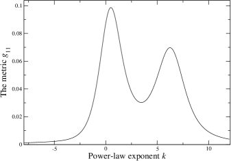
Figure 1: The only metric component, $g_{11}$, for a single power-law SGWB plotted as a function of $k$. The template spacing is a minimum near the global maximum at $k=0.5000^{+0.0625}_{-0.0625}$.

The only metric component for the above SGWB signal is readily deduced from Eq. (28) as

$$g_{11}(k)=\frac{1}{2}\left[\alpha(2)-\alpha^{2}(1)\right]\ \ ,$$ (30)

which has the following properties: First, the Cauchy-Schwarz inequality can be used to prove that $g_{11}(k)$ is non-negative for all real $k$ boseCalib . Second, Eqs. (28) and (29) show that it is dependent on $k$, which is confirmed by Fig. 1. This implies that for the optimal coverage of the $k$-space the template-spacings must be chosen to vary in step with the $g_{11}(k)$ values. The template spacing is a minimum at the global maximum of $g_{11}(k)$ (at $k\simeq 0.5$), and is:

$$dk=0.637\left(\frac{1-{\rm MM}}{0.01}\right)^{1/2}\ \ ,$$ (31)

where ${\rm MM}$ is the minimal match required by an observer between the discretely spaced templates and a signal. Typically, ${\rm MM}$ is set equal to 97%. But we find above that $dk$ is as large as 0.637 for a minimal match as high as 99%, as is evident in Fig. 2.

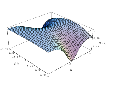
Figure 2: The ambiguity function, $M(k,\delta k)$, for a single power-law SGWB plotted as a function of $k$ and the mismatch, $\delta k$. For any given $k$, the function attains the maximum possible value of unity when $\delta k=0$. And for any given $\delta k$, the function is a minimum at $k=0.5000^{+0.0625}_{-0.0625}$, which is consistent with the behavior of the metric depicted in Fig. 1 numericalAmbiguityFunctions .

If one were to choose the template-spacing to be uniformly equal to the above value and, therefore, err on the side of over-covering the parameter space, then the number of templates required for a search with $k\in[-4,4]$ and a minimal match of at least 99% is kValues

$$N={\rm Ceiling}\left[\frac{k_{\rm max}-k_{\rm min}}{0.637}\right]=13\ \ ,$$ (32)

which is easily implementable in real time on the data of a detector pair.

.0.2 Broken power-laws

A likely character of $\Omega_{\rm GW}(f)$ will be in the form of a broken power-law (BPL) in frequency Ungarelli:2003ty ,

$$\small{\Omega_{\rm GW}(f)=\Omega_{0}\Bigg{[}\Theta\left(1-\frac{f}{f_{p}}\right)\left(\frac{f}{f_{p}}\right)^{k_{-}}+\Theta\left(\frac{f}{f_{p}}-1\right)\left(\frac{f}{f_{p}}\right)^{k_{+}}\Bigg{]}\ \ ,}$$ (33)

where $k_{-}\geq 0$, $k_{+}\leq 0$ are real power-law exponents, and the peak frequency, $f_{p}$, and $\Omega_{0}$ are positive-definite real constants. The first three are intrinsic search parameters, which define the three-dimensional parameter space, $\mbox{\boldmath$\vartheta$}=(f_{p}/f_{p0},k_{-},k_{+})$. Here $f_{p0}$ is an arbitrary reference frequency chosen large enough so that $\delta f_{p}/f_{p0}$ is small and the ${\cal O}\left(\delta\mbox{\boldmath$\vartheta$}^{3}\right)$ terms in Eq. (13) are indeed negligible.

We calculate the ambiguity function for the templates in Eq. (25), with the above $\Omega_{\rm GW}(f)$, and compute the metric from its second derivatives using Eq. (14). These derivatives now involve the following integrals of the logarithm and different powers of $f$:

$$D := \Bigg{[}\int_{f_{-}/f_{p}}^{1}dx\frac{\gamma^{2}(f_{p}x)x^{2k_{-}-6}}{P_{A}(f_{p}x)P_{B}(f_{p}x)}$$

$$\>\>+\int_{1}^{f_{+}/f_{p}}dx\frac{\gamma^{2}(f_{p}x)x^{2k_{+}-6}}{P_{A}(f_{p}x)P_{B}(f_{p}x)}\Bigg{]}^{-1}\ \ ,$$

$$\alpha_{\pm}\left(n\right) := \mp D\int_{f_{\pm}/f_{p}}^{1}dx\frac{\gamma^{2}(f_{p}x)x^{2k_{\pm}-6}\left[\ln x\right]^{n}}{P_{A}(f_{p}x)P_{B}(f_{p}x)}\ \ ,$$

$$\beta_{\pm}\left(n\right) := \mp Dk_{\pm}^{n}\int_{f_{\pm}/f_{p}}^{1}dx\frac{\gamma^{2}(f_{p}x)x^{2k_{\pm}-6}}{P_{A}(f_{p}x)P_{B}(f_{p}x)}\ \ ,$$

$$\beta(n) := \beta_{-}(n)+\beta_{+}(n)\ \ ,$$ (34)

where the dependence of $D$, $\alpha_{\pm}(n)$, $\beta_{\pm}(n)$, and $\beta(n)$ on the detector indices $A$ and $B$ is implicit.

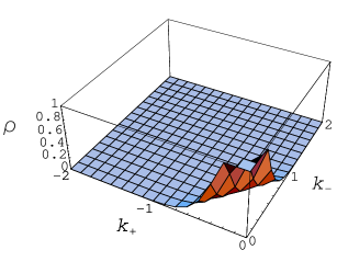
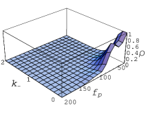
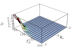
Figure 3: The template-density $\rho$ (normalized here to have a maximum value of 1) for a BPL parameter-space plotted as a function of $k_{\pm}$ and $f_{p}$, two variables at a time. The fixed parameters in these plots are (clockwise from top) $f_{p}=50$Hz, $k_{-}=0.125$ and $k_{+}=-0.125$.

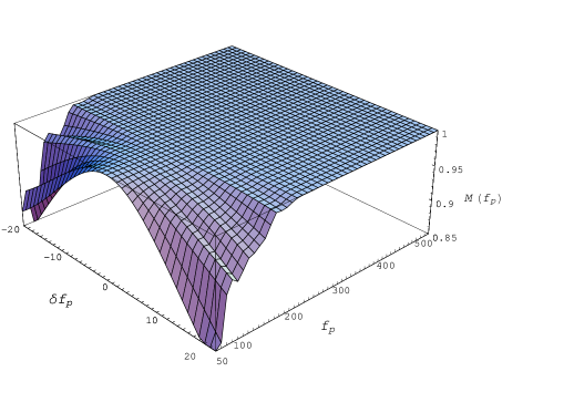
Figure 4: The ambiguity function, $M(\mbox{\boldmath$\vartheta$},\delta\mbox{\boldmath$\vartheta$})$, for a broken power-law SGWB plotted as a function of $f_{p}$ and the mismatch, $\delta f_{p}$ (both in Hz). Here, we set $k_{\pm}=\mp 2$ and $\delta k_{\pm}=0$. Note how quickly $M$ asymptotes to a value of unity for large $f_{p}$, implying a small number of templates for $f_{p}\stackrel{{\scriptstyle\Large{>}}}{{\small{\sim}}}200$Hz. The ambiguity function is within 99% for: (a) $f_{p}\in[50,120]$Hz, if $\delta f_{p}\leq 4$Hz, (b) $f_{p}\in(120,150]$Hz, if $\delta f_{p}\leq 10$Hz, and (c) $f_{p}>150$Hz, if $\delta f_{p}\leq 20$Hz.

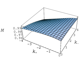
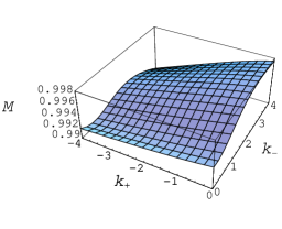
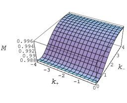
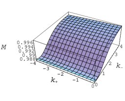
Figure 5: $M(\mbox{\boldmath$\vartheta$},\delta\mbox{\boldmath$\vartheta$})$ for BPL spectra plotted as a function of $k_{+}$ and $k_{-}$ for four values of $f_{p}=$ 50, 100, 190, 450Hz (clockwise from top left). The mismatch values are $\delta k_{\pm}=0.25$ and $\delta f_{p}=2.5$Hz. As $f_{p}$ increases, note how little $M$ varies with $k_{+}$ (for any given $k_{-}$). This is indicative of the template spacings being larger along $k_{+}$ than along $k_{-}$. This is expected since most of the contribution to the CC statistic arises at lower frequencies, where the $k_{-}$ index has support (especially, when $f_{p}\stackrel{{\scriptstyle\Large{>}}}{{\small{\sim}}}200$Hz).

The six independent components of the symmetric metric on the three-dimensional parameter space, $(f_{p}/f_{p0},k_{-},k_{+})$, are:

$$g_{00} = \frac{1}{2}\left(\frac{f_{p0}}{f_{p}}\right)^{2}\left[\beta(2)-\beta^{2}(1)\right]$$

$$g_{11} = \frac{1}{2}\left[\alpha_{-}(2)-\alpha_{-}^{2}(1)\right]\ \ ,$$

$$g_{22} = \frac{1}{2}\left[\alpha_{+}(2)-\alpha_{+}^{2}(1)\right]\ \ ,$$

$$g_{01} = \frac{1}{2}\left(\frac{f_{p0}}{f_{p}}\right)\left[\beta(1)-k_{-}\right]\alpha_{-}(1)\ \ ,$$

$$g_{02} = \frac{1}{2}\left(\frac{f_{p0}}{f_{p}}\right)\left[\beta(1)-k_{+}\right]\alpha_{+}(1)\ \ ,$$

$$g_{12} = -\frac{1}{2}\alpha_{-}(1)\alpha_{+}(1)\ \ ,$$ (35)

where the parameter vector components were taken to be $\vartheta^{0}=f_{p}/f_{p0}$, $\vartheta^{1}=k_{-}$, and $\vartheta^{2}=k_{+}$. Once again it is clear that the metric is dependent on the parameters, as confirmed by Fig. 3. Thus, the template spacing for a fixed minimal match is not uniform inflateBPL .

  

  

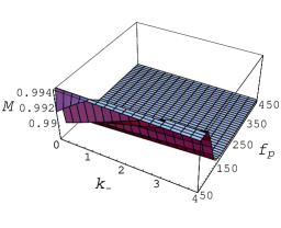
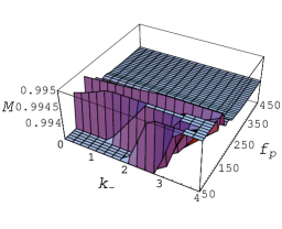
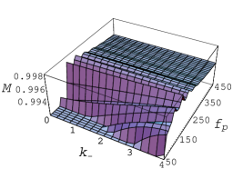
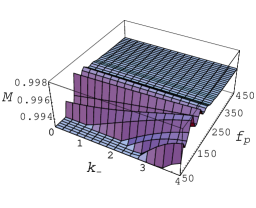
Figure 6: $M(\mbox{\boldmath$\vartheta$},\delta\mbox{\boldmath$\vartheta$})$ for a broken power-law SGWB plotted as a function of $k_{-}$ and $f_{p}$ for four values of $k_{+}=$ -4, -2, -1, 0 (clockwise from top left). The mismatch values are $\delta k_{\pm}=0.25$ and $\delta f_{p}=2.5$Hz.

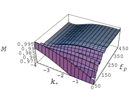
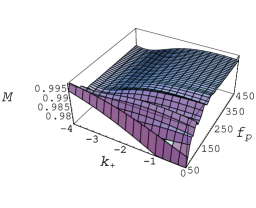
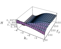
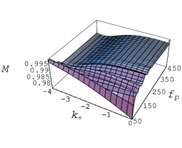
Figure 7: $M(\mbox{\boldmath$\vartheta$},\delta\mbox{\boldmath$\vartheta$})$ for a broken power-law SGWB plotted as a function of $k_{+}$ and $f_{p}$ for four values of $k_{-}=$ 0, 1, 2, 4 (clockwise from top left). The mismatch values are $\delta k_{\pm}=0.25$ and $\delta f_{p}=2.5$Hz.

The number of templates, $N$, can be estimated from the above metric by dividing the parameter space volume,

$$V=\int d^{3}\vartheta\sqrt{\det\|g_{\mu\nu}\|}\ \ ,$$ (36)

by the volume of a unit cell in three-dimensional space, $v=(2\sqrt{(1-{\rm MM})/3}~{})^{3}$ Owen96 . We numerically compute the above volume and find that

$$N\simeq 250\left(\frac{1-{\rm MM}}{0.03}\right)^{-3/2}\ \ ,$$ (37)

where we again err on the side of over-coverage by relaxing the numerical computation to allow for ${\rm MM}\geq$ 97%. The parameter-dependence of the template density, $\rho=\sqrt{\det\|g_{\mu\nu}\|}/v$, is illustrated in Fig. 3. The above value of $N$ is consistent with the near-unity value of the ambiguity function shown in Figs. 4-7 for template-spacings as large as $\delta k_{\pm}=0.25$ and $\delta f_{p}=2.5$Hz.

It has been projected in Ref. Allen:1997ad that LIGO-I and Advanced LIGO may succeed in placing upper limits on $\Omega_{0}$ of the order of $5\times 10^{-6}$ and $5\times 10^{-11}$, respectively, for the $k=0$ SPL spectrum. The first science run at LIGO already demonstrated successfully the application of a single template (i.e., the $k=0$ case of SPL) on the data from the LIGO detector pairs to obtain bounds on $\Omega_{0}$ ligoS1 ; Bose:2003nb . With the upcoming science runs at LIGO, the sensitivities are fast approaching closer to the designed target so as to make the first upper limit given above realizable in the near future. This progress necessitates the availability of techniques and templates to look for a variety of proposed astrophysical and cosmological SGWBs in the ever-so sensitive data. This paper addresses this issue for the latter category of signals, which assumes the background to be isotropic and unpolarized. The former case of an astrophysical background will be discussed elsewhere boseASGWB .

References

(1)
M. Maggiore,
Phys. Rept. 331, 283 (2000)
[arXiv:gr-qc/9909001]. Also see the references therein.
(2)
C. Ungarelli and A. Vecchio,
Class. Quant. Grav. 21, S857 (2004)
[arXiv:gr-qc/0312061].
(3)
B. Allen and S. Koranda,
Phys. Rev. D 50, 3713 (1994)
[arXiv:astro-ph/9404068].
(4)
S. Bose and L. P. Grishchuk,
Phys. Rev. D 66, 043529 (2002)
[arXiv:gr-qc/0111064].
(5)
V. M. Kaspi, J. H. Taylor and M. F. Ryba,
Astrophys. J. 428, 713 (1994).
(6).
E. W. Kolb and M. Turner, The Early Universe, Frontiers in Physics
(Addison-Wesley, Reading, MA, 1990).
(7)
V. Ferrari, S. Matarrese and R. Schneider,
Mon. Not. Roy. Astron. Soc. 303, 258 (1999)
[arXiv:astro-ph/9806357].
(8)
P. L. Bender et al. ”LISA: A cornerstone mission for the observation of
gravitational waves: System and technology study report” ESA-SCI(2000)11 (2000).
(9)
P. L. Bender and D. Hils,
Class. Quant. Grav. 14, 1439 (1997).
(10)
A. Krolak, M. Tinto and M. Vallisneri,
Phys. Rev. D 70, 022003 (2004)
[arXiv:gr-qc/0401108].
(11)
A. Rogan and S. Bose,
Class. Quant. Grav. 21, S1607 (2004)
[arXiv:gr-qc/0407008].
(12)
C. W. Helstrom, Statistical Theory of Signal Detection (Pergamon Press,
London, 1968).
(13)
P. Saulson, “Fundamentals of Interferometric Gravitational Wave Detectors,”
(World Scientific Publishing Company, 1994).
(14)
B. J. Owen, Phys. Rev. D 53, 6749 (1996). (gr-qc/9511032)
(15)
S. Bose, “Effects of calibration inaccuracies on matched filtering:
Applications in gravitational-wave detection and parameter estimation,”
in preparation.
(16)
P. Dennery and A. Krzywicki, “Mathematics for physicists,” Harper & Row,
New York (1967).
(17)
B. Allen and J. D. Romano,
Phys. Rev. D 59, 102001 (1999)
[arXiv:gr-qc/9710117].
(18)
S. Bose, “Search templates for gravitational-wave backgrounds
from astrophysical sources,” in preparation.
(19)
N. Christensen,
Phys. Rev. D 46, 5250 (1992).
(20)
E. E. Flanagan, Phys. Rev. D 48, 2389 (1993) [arXiv:astro-ph/9305029].
(21)
A. Lazzarini et al.,
Phys. Rev. D 70, 062001 (2004)
[arXiv:gr-qc/0403093].
(22)
A. Lazzarini and R. Weiss, “LIGO Science Requirements Document,” LIGO
technical document no. LIGO-E950018-02-E (1996).
(23)
All plots of the ambiguity function in this paper are computed numerically and
give a more accurate, but not appreciably different, value of than
what can be estimated from Eq. (13).
(24)
The range of values that an observer is interested in searching for will
depend on the availability of models predicting SGWBs with those values and
the noise spectral profiles of the detector pair. The range chosen
here is for illustrative purposes. However, the metric expression given here
can be applied to estimate the required number of templates for a wider range of
values.
(25)
Note that the slow-roll inflationary SGWB spectrum will appear in the bandwidth
of LISA- or LIGO-type detectors as a
SPL spectrum, and will be indistinguishable from a BPL spectrum
if either and
or and . In this limited sense, the SRIM spectrum
can be construed as a special case of the BPL.
(26)
B. Abbott et al., Phys. Rev. D69, 122004 (2004).
(27)
S. Bose et al.,
Class. Quant. Grav. 20, S677 (2003).