Studying the Variation of the Fine Structure Constant Using Emission Line Multiplets

Abstract

As an extension of the method by Bahcall et al. (2004) to investigate the time dependence of the fine structure constant, we describe an approach based on new observations of forbidden line multiplets from different ionic species. We obtain optical spectra of fine structure transitions in [Ne III], [Ne V], [O III], [OI], and [SII] multiplets from a sample of 14 Seyfert 1.5 galaxies in the low-z range 0.035 $<z<0.281$. Each source and each multiplet is independently analyzed to ascertain possible errors. Averaging over our sample, we obtain a conservative value $\alpha^{2}(t)/\alpha^{2}(0)$ = 1.0030$\pm$0.0014. However, our sample is limited in size and our fitting technique simplistic as we primarily intend to illustrate the scope and strengths of emission line studies of the time variation of the fine structure constant. The approach can be further extended and generalized to a ”many-multiplet emission line method” analogous in principle to the corresponding method using absorption lines. With that aim, we note that the theoretical limits on emission line ratios of selected ions are precisely known, and provide well constrained selection criteria. We also discuss several other forbidden and allowed lines that may constitute the basis for a more rigorous study using high-resolution instruments on the next generation of 8 m class telescopes.

1 Introduction

The variation of the fine structure constant $\alpha$ =$e^{2}/4\pi\epsilon_{0}hc$ is of fundamental interest in cosmology. However, if there is a variation of the fundamental constants by time, the effect will be very small. Recent laboratory measurements using $\rm{}^{171}Yb^{+}$ by Peik et al. (2004) give an upper limit of 2$\times 10^{-15}\rm yr^{-1}$ resulting in a change of $\alpha$   of the order of $10^{-5}$ in 10 Gyrs. In order to measure this effect using astronomical observations, they have to be performed with high-redshift objects. Therefore the lines to be studied need to manifest themselves as strong features in the spectrum. The most common methods are measurements of high-redshift Ly$\alpha$ forest metal absorption lines. Among the first ones was the “alkali-doublet method” (e.g. Bahcall et al., 1967) with transitions from the singlet ground level to the two fine structure doublets in alkali-like systems, such as the recent study of C IV and Si IV systems using a QSO spectra from UVES (Martinez Fiorenzano et al., 2003). The most extensive body of work in recent years is described by Murphy et al. (2003) (and references therein), who have considerably extended absorption line studies to a relatively large number of multiplets in heavy atomic systems, including the iron group elements. Their “many multiplet method” represents ‘an order of magnitude increase in precision’ over the alkali doublet method and uses Lyman$\alpha$ forests of Quasars (Dzuba et a., 1999a, b; Webb et al., 1999, 2002; Murphy et al., 2001a, b, e.g.).

Recently, as an alternative Bahcall et al. (2004) described an extensive analysis of forbidden fine structure lines of the well known nebular [O III] doublet at 5006.84 and 4958.91 Å. These lines have the great advantage that they are extremely bright and nearly ubiquitous in the optical spectra of H II regions in most sources. The approach by Bahcall et al. (2004) involved the study of archived spectra of 3,814 quasars from the large database of the Sloan Digital Sky Survey (SDSS York et al., 2000). They devised elaborate algorithms based on stringent selection criteria to search for and obtain a standard spectral sample of 42 quasars, as well as alternate samples based on variants of the selection criteria. Among these criteria are fits to the line profiles and line ratios. Since both lines originate within the same upper level, their line profiles must be similar and their line ratios depend only on intrinsic atomic properties, the energy differences between the fine structure levels and corresponding spontaneous decay Einstein A-coefficients, i.e. independent of external physical conditions such as the density, temperature, and velocities. Bahcall et al. (2004) also noted that other similar forbidden multiplets of [Ne V] and [Ne III] could be exploited for emission line studies, but they are likely to be weaker than the [O III] by an order an magnitude in typical quasar spectra.

The quasar absorption line many-multiplet method has clear advantages: because it measures the Ly$\alpha$ forest of high-redshift systems at observed optical wavelengths its look-back time into the Universe’s history is long. It also uses many line pairs to measure any time dependence of $\alpha$ and provides good statistics to minimize systematic errors of the measurements of an individual line pair. However, the method has some disadvantages: It is observationally expensive, requiring very high resolution, like $\lambda/\Delta\lambda\geq$50000 using high-resolution Echelle spectrographs and long exposure times on large telescopes (e.g. Murphy et al. (2003)). Also the line pairs measured by this method are from different atomic stages suggesting that they are not necessarily formed in the same regions. Another disadvantage is that the large number of absorption lines in Ly$\alpha$ forest systems make it difficult for the correct identification of the lines; many lines are blended requiring multi-Gaussian fits to the line blends in order to determine the wavelengths. Based on high-resolution Keck spectra of several different samples of quasars, Murphy et al. (2003) report a ’highly significant’ value of $\Delta\alpha/\alpha_{0}$ = $-0.57\pm 0.10\times 10^{-5}$. In contrast the statistically invariant result by Bahcall et al. (2004) yields a value of $0.7\pm 1.4\times 10^{-4}$. An extensive discussion of relative problems and advantages of various methods is given, among others, by Bahcall et al. (2004) and Levshakov (2003).

The optical [O III] forbidden emission lines $\lambda\lambda$4959, 5007Å  studied by Bahcall et al. (2004) are relatively easy to measure in most AGN, (except in Narrow-Line Seyfert 1 galaxies (NLS1s) in which these lines can be very weak and contaminated by strong FeII emission (e.g. Boroson & Green, 1992; Grupe, 2004; Sigut & Pradhan, 2003, 2004). The observations can be performed with lower resolution Spectrographs and smaller telescopes. Bahcall et al. (2004) presented a sample of 44 AGN carefully selected from the SDSS and measured the wavelength shifts between the [OIII]$\lambda\lambda$4959,5007Å  lines. The disadvantage of this method is that it only uses one line pair and it can only be used in the optical wavelength range for objects with redshifts z$<$0.8 before the [OIII]$\lambda$5007Å line is shifted out of the observable optical wavelength range and NIR spectroscopy is required for objects of higher redshift.

In this paper we generalize the emission line method outlined by Bahcall et al. (2004) by incorporating, in principle, the main advantage of the many-multiplet absorption line method. However, there are other key differences with Bahcall et al. (2004). We carry out new observations of quasars and Seyfert 1 galaxies, rather than analyze existing data. This obviates the need for complex search routines that forms the bulk of the analysis of the SDSS data by Bahcall et al. (2004). We expect better accuracy since objects are pre-selected from previous observations for good quality optical spectra to enable optimum analysis. Since the redshifts are known a priori, we know the approximate positions of the well known forbidden lines. Theoretically known line ratios (discussed in the next section) offer an additional indication of the quality of the spectra.

This many-multiplet emission line method not only allows us to measure more than one line pair per object and gives a more secure result, it also, once established, opens the possibility of observing objects of higher redshift in the optical wavelength range. Another purpose of our observing run was to test whether it is feasible to use a 2m class telescope with a medium resolution spectrograph to get enough accuracy to perform a measurement of the time variation of the fine-structure constant $\alpha$. While the availability of observing time at large 8-10m class telescope is very limited, many institutions have access to 2-3m small/medium size telescopes. In this work we focus on laying out the framework for general emission line analysis, potentially leading to future studies using the many-multiplet emission line method, with a relatively small sample. However, we discuss a variety of further extensions.

This paper is organized as follows: in § 2 we describe the theoretical background of the fine structure separation of the LS multiplets, in § 3 we describe the spectroscopic observations at MDM observatory, in § 4 the results are presented, and discussed in § 5 usually in the context of systematical errors in the wavelength calibration. Finally, we note a few main features of our method in the concluding section 6.

2 Theory

Relativistic electron interactions lead to fine structure separation of LS-coupling multiplets. The level energies may be expanded in terms of a non-relativistic term and relativistic terms in powers of $\alpha$ (Bethe & Salpeter, 1977). Although the exact formulation is predicated on the Dirac theory (Grant, 1996), Breit formulated the generalized interaction for non-hydrogenic systems that leads to the so called Breit-Pauli approximation for the total electronic Hamiltonian as a sum of one-body and two-body operators, referred to as the non-fine structure and fine structure terms (Drake, 1996; Frose-Fisher, 1996). The leading relativistic terms, such as the spin-orbit coupling, are of the order of $\alpha$ ²; higher order terms are orders of magnitude smaller. Forbidden lines arise from transitions between LS states of the same electronic configuration of an atomic system, usually the ground configuration. Fine structure components of a forbidden LS multiplet are separated by $\Delta$E $\propto$ $\alpha$ ². The time dependence of $\alpha$ therefore should manifest itself in different energy or wavelength separations at different cosmological epochs.

2.1 Forbidden Lines and $\alpha$ (t)

Bahcall et al. (2004) show that, for two lines from a forbidden multiplet, the ratio

$$R(t)=\frac{\lambda_{2}-\lambda_{1}}{\lambda_{2}+\lambda_{1}},$$ (1)

at a cosmological time t is related to the ratio at the present epoch t = 0 by

$$\frac{R(t)}{R(0)}=\frac{\alpha^{2}(t)}{\alpha^{2}(0)},$$ (2)

where the RHS is a measure of the variation in $\alpha$ as a function of the ’cosmological look-back time’ t. Wavelength separation between a pair of well defined forbidden lines may thus be used as a ‘chronometer’ provided its value at an earlier cosmological epoch differs from that at present.

As mentioned, Bahcall et al. (2004) had already suggested the possibility of extending this study with other emission line pairs, such as [Ne V]$\lambda\lambda$3346,3426Å  and [Ne III]$\lambda\lambda$3869,3968Å. The left panel of Figure 1 shows the schematic diagram of four ionic species ([NeIII], [NeV], [OIII], and [OI]) and the two lines ${}^{1}D_{2}\rightarrow^{3}P_{2}$ and ${}^{1}D_{2}\rightarrow^{3}P_{1}$. It might be noted that while [O I] and the isoelectronic ions C-like [O III] and [Ne V] have the ground level $2p2(^{3}P_{0})$, the O-like [Ne III] has a different atomic structure with the ground level $2p4(^{3}P_{2})$. In addition we consider the well known nebular doublet lines [OII] and [SII] due to transitions ${}^{2}D^{o}_{5/2},^{2}D^{o}_{3/2}\longrightarrow^{4}S^{o}_{3/2}$. The atomic transitions within the ground configuration correspond to magnetic dipole (M1) and the much smaller electric quadrapole (E2) interactions. The wavelengths and atomic transitions of the [NeIII], [NeV], [OIII], [OI], and [SII] lines are given in Table 1.

2.2 Line Ratios

Subsequent analysis of different emission line multiplets rests on the basic property of the ratio of lines originating in the same upper level. For such a 3-level system the theoretical emissivity ratio of line intensities is

$$LR=\frac{N_{3}A_{31}h\nu_{31}}{N_{3}A_{32}h\nu_{32}}.$$ (3)

The upper level population is the same for both lines, and the $R_{\epsilon}$ depends only the intrinsic atomic parameters, the transition rates or A-values, and the energy differences. Generally, for forbidden lines, the A-values are obtained from sophisticated theoretical calculations, whereas the energies are available from laboratory measurements. While the prime resource for both quantities is the on-line National Institute of Standards and Technology (NIST) compilation (www.nist.gov), some of the NIST data for A-values is not quite up-to-date. The differences may be slight but quite significant. Table 2 shows the line ratios for the 5 ions and respective multiplets using both the NIST data and the most recent calculations.

In their work Bahcall et al. (2004) quote the line ratio for the [O III] $\lambda\lambda$4959,5007Å  line using NIST values as 2.92, as opposed to their measured value of 2.99 $\pm$ 0.02. However, the 2.92 is the ratio of the A-values alone, not the emissivity ratio above; taking account of the energy differences the NIST tabulations yield 2.89. While this is in even worse agreement with the measured ratio, the most recent calculations of A-values by Storey & Zeippen (2000) yields a significantly better theoretical value of 2.98, in agreement with Bahcall et al. (2004). The crucial difference between the Storey & Zeippen (2000) results and previous calculations (such as by Galavis et al., 1997) is taking account of higher order relativistic corrections to the magnetic dipole M1 operator (Drake, 1971; Eissner & Zeippen, 1981). The above discussion emphasizes the need for extremely accurate atomic calculations including all relevant relativistic effects, as well as a well optimized configuration interaction expansion, both of which are important to obtain precise A-values for fine structure transitions.

The actual value of the forbidden line ratio may be of decisive importance in spectral identification and analysis of observational datasets, and they indicate the extent of line blending and signal-to-noise ratio. It is therefore instructive to examine further (with a view towards future work as well) the line ratios of interest in this work. For the forbidden lines in the left panel of Figure 1 the dominant contribution is from the M1 operator (the E2 contribution is about 3 orders of magnitude smaller). In the LS coupling limit, as the magnetic interaction goes to zero, the ratio of the line strengths $S(^{1}D_{2}-^{3}P_{2})/S(^{1}D_{2}-^{3}P_{1})$ = 3 (Storey & Zeippen, 2000). The A-values however involves the energy differences as well, i.e. $A(^{1}D_{2}-^{3}P_{2})/A(^{1}D_{2}-^{3}P_{1})$ = 3 $E(^{1}D_{2}-^{3}P_{2})3/E(^{1}D_{2}-^{3}P_{1})3$. The line ratio (Eq. 3) deviates from the value of 3, in accordance with the magnitude of the magnetic interaction. It is highly fortuitous that for O III this ratio is in fact 3, as noted by Bahcall et al. (2004) and (Storey & Zeippen, 2000). But for other ions there is significant deviation, as seen in Table 2. We do not give line ratios for the [SII] lines because their line ratios depends strongly in the gas temperature (e.g. Osterbrock,, 1989). We derive this ratio for all three ions using 4 different datasets available in literature. While all sets of line ratios agree to within few percent, we envisage that this level of difference could turn out to be crucial in analyzing large datasets, with line ratios measured and calculated to better than 1% accuracy.

In addition to the ions with ground state fine structure levels discussed above, there are well known pairs of lines in ions with excited state fine structure levels, such as the doublet forbidden lines [O II] and [S II] at $\lambda\lambda(\AA)$ = (3728.8/3726.0) and (6716.5/6730.8) respectively (right panel of Figure 1), observed from many H II regions and AGN (Osterbrock,, 1989; Pradhan, 1976). While collisional coupling leads to variations in line ratios dependent on electron density, the limiting values of these ratios are precisely known. For example, the low density line ratio LR (N${}_{e}\longrightarrow 0$) = 1.5 for both [O II] and [S II]: the ratio of the statistical weights of the upper levels in associated pair of transitions (${}^{2}D^{o}_{5/2},^{2}D^{o}_{3/2}\longrightarrow^{4}S^{o}_{3/2})$. The high density limit is given by

$$LR(N_{e}\rightarrow\infty)=\frac{g(^{2}D^{o}_{5/2})}{g(^{2}D^{o}_{3/2})}\frac{A((^{2}D^{o}_{5/2}-^{4}S^{o}_{3/2})}{A(^{2}D^{o}_{3/2}-^{4}S^{o}_{3/2})},$$ (4)

and is = 0.35 for [O II] (Zeippen, 1987) and 0.44 for [S II] (Mendoza and Zeippen, 1982). Studies of ionized gaseous nebulae show no known cases of deviations from these ’canonical’ limits (Wang et. al., 2004). Whereas the wavelength separation between the [O II] doublet is possibly too small to be resolved in AGN, the [S II] doublet is easily observed and resolved, as in the present exploratory work.

3 Observations and data reduction

We observed a small sample of 14 Seyfert 1.5 galaxies with the 2.4m Hiltner telescope at MDM observatory at Kitt Peak, Arizona, for 5 nights from 2003-10-16 to 2003-10-21 to cover the [NeV], [NeIII] and [OIII] lines — the blue part of the optical spectrum — and 3 nights starting 2004-10-10 to observe the [OI] and [SII] doublets towards the red part of the spectrum. (Table 3). All spectra were taken with the OSU CCDS spectrograph with the 600 grooves/mm grating in first order. The slit width of the 2003 run was 1${}^{{}^{\prime\prime}}$ corresponding to a spectral resolution in FWHM of about 2Å. The weather conditions during the whole run were excellent with mostly photometric conditions. The slit position was normally at E-W for the spectra in the 4000-7000Å  range, but all spectra in the blue were observed in N-S direction to compensate for refraction losses in the earth’s atmosphere. During the 2004 run the weather conditions were clear but suffered from rather bad seeing. Most observations during the 2004 run were performed with slit widths of 1.5${}^{{}^{\prime\prime}}$ and 2.0${}^{{}^{\prime\prime}}$. The slit was oriented in N-S direction for all 2004 observations.

The total exposure times per spectrum are given in Table 3. Each spectrum consists of 2-4 single spectra which were combined after going through all data reduction steps. For each individual spectrum a wavelength calibration spectrum was taken. For the wavelength calibration we used a Hg lamp for the 3400-4300Å range, Xe for the 4100-5100Å range, Ne for the 5100-6000Å  range, and Ar for the 4900-5900Å and all observation with $\lambda>$6000Å. For the flat field correction the CCDS spectrograph only allows internal flats. To perform a flat field correction we used an average of 10 flats. We used standard stars BD+28-4211, Feige 110, G191 B2B, and Hiltner 600 for the flux calibration. The data reduction was performed with the ESO MIDAS data reduction and analysis package version 01FEBpl1.4.

The wavelength measurements were performed by fitting a Gaussian at 80% of the line peak in order to avoid possible line asymmetries that can occur at lower parts of an emission line. Line fluxes were measured by integrating over the whole line using the MIDAS command integrate/line. In order to estimate the error of the data reduction, the data were reduced and analyzed independently by D.G. and S.F..

4 Results

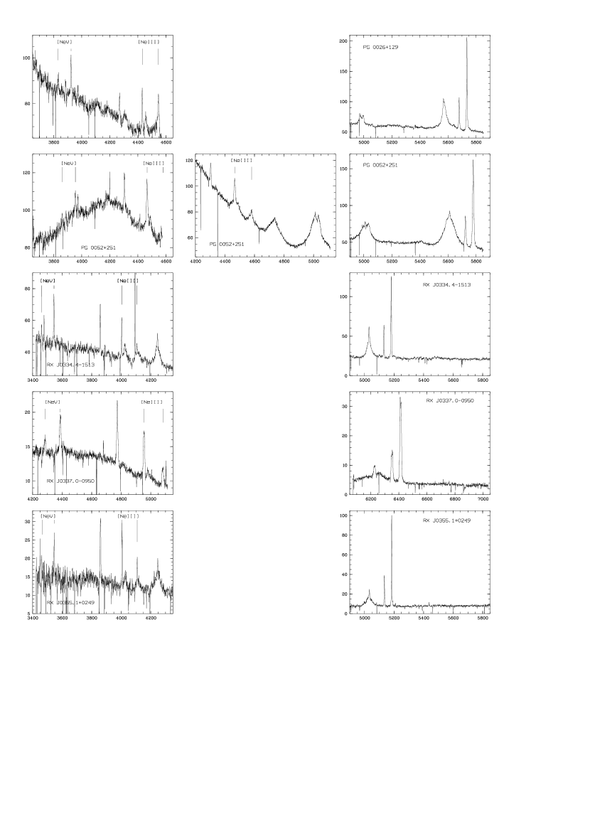
Figure 2: Optical spectra of the [NeV], [NeIII], and [OIII] regions

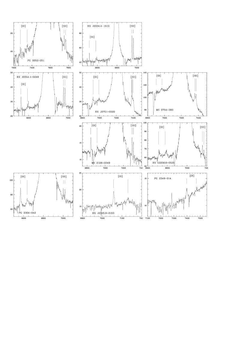
Figure 3: Optical spectra of the [OI] and [SII] line regions

Figure 2 displays the optical spectra of the [NeV0, NeIII], and [OIII] line regions of the objects sorted by RA as given in Table. 3. As shown in Figure 2 in most of the sources the lines are clearly present and have enough S/N that their wavelengths and fluxes can be measured. The spectra of the [OI] and [SII] lines taken in October 2004 are shown in Figure 3. In most cases the [SII] lines are clearly present. However, the [OI]$\lambda$6363 line in most cases is too noisy to allow accurate measurements of the wavelength.

Table 4 lists the line flux of the [OIII]$\lambda$5007Å  line and the line ratios. In general, the [NeV]$\lambda$3426 and [NeIII]$\lambda$3869 line are about 1/10th of the [OIII]$\lambda$5007 line. Table 5 lists the observed wavelengths of the [NeV], [NeIII], [OIII], [OI], and [SII] lines.

For the low-redshift AGN in our sample with a maximum look-back time of about 2 Gyrs we would expect a maximum change of $\alpha$ of 4$\times 10^{-6}$ regarding the the laboratory measurements of Peik et al. (2004). Therefore the expected ratio $\alpha^{2}(t)/\alpha^{2}(t)$ maximum is 1.000008. Every deviation from this value gives us a handle on the quality of our measurements. Table 6 lists the ratios of $\alpha^{2}(t)/\alpha^{2}(0)$ which are equal to the R(t)/R(0) ratio, with R(t) = $(\lambda 2(t)-\lambda 1(t))/(\lambda 1(t)+\lambda 2(t)$ and R(0) are given by the laboratory wavelengths as R(0)([NeV])=1.1814, R(0)([NeIII])=12.597, R(0)([OIII])=4.80967, R(0)([OI])=5.011971, and R(0)([SII])=1.0690657 $\times 10^{-3}$ (for all lines). Table 6 also summarizes the mean values of $\alpha^{2}(t)/\alpha^{2}(0)$ for each object as well the sample averaged value. In general, we find results with the lowest error estimates from the [NeIII] lines owing to their wide wavelength separation, whereas the values obtained from the [SII] lines suffer in precision from their small splitting. Clearly, the lines with the highest SNR offer the best possibilities to constrain their centers, making the original approach based upon the [OIII] doublet so effective.

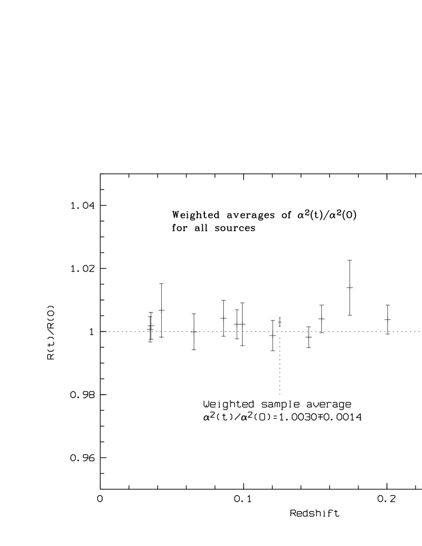
Figure 4: Redshift vs. $\alpha^{2}(t)/\alpha^{2}(0)$

Even though we are not attempting to measure a redshift dependence of the fine structure constant $\alpha$ by redshift due to the low redshift of the AGN in our sample, Figure 4 displays the redshift vs. $\alpha^{2}(t)/\alpha^{2}(0)$ diagram. As expected we do not see any significant deviation from 1.0000.

5 Discussion

As mentioned before, it is beyond the scope of this paper to measure the time dependence of the fine structure constant $\alpha$ with adequate precision. The redshifts of the objects in our sample only cover a range between 0.034-0.281. The look-back time of an object of z=0.28 is of the order of $\approx$ 3 Gyrs. With the upper limit of a possible change of $\alpha$  measured by Peik et al. (2004) of $\Delta\alpha=2\times 10^{-15}$ yr^-1 we would expect an upper limit of $\Delta\alpha=6\times 10^{-6}$, which implies that a two orders of magnitude improvement is needed over what we can achieve from our current data set.

For measuring any redshift dependence of the fine structure constant $\alpha$  , estimates of the accuracy in determining the wavelengths of the line doublets are absolutely crucial. Evaluating $\alpha^{2}(t)/\alpha^{2}(0)$ we do not need to rely on absolute wavelength calibrations, but relative wavelengths ratios. However, the issues that are important are: First, the stability of the wavelength calibration between two lines in a line pair, which can be separated up to $\approx$100Å  in the case of [NeIII], and second, the ability to determine the line centroids. While the first issue is relatively safe for the [OIII], [OI] and [SII] lines, because their separation is rather small and the wavelength calibration is very secure due to the large number of calibration lamp lines, the situation is more difficult for the [NeIII] and [NeV] lines. Not only that the separation between the two lines in the [NeIII] and [NeV] line pairs are about 100Å, also the wavelength calibration in the blue using the CCDS spectrographs suffers from a lack of enough calibration lamp lines. The CCDS spectrograph only has a Hg lamp providing just 5 calibration lines throughout the blue/UV wavelength range. Certainly, a Th/Ar lamp could improve our ability to provide for a more stable calibration in this regime. The situation for these line pairs would also improve for objects of higher redshift as the observed features shift into the longer wavelength regime where the calibration is better. Furthermore, we indicate that the abundant night-sky lines upwards from 6500 Å could be used as additional calibrators to measure small-scale flexures as already indicated by (Bahcall et al., 2004).

Measuring the center of the lines depends on a variety of factors: the spectral resolution and dispersion of the instrument, the pixel sampling, the signal-to-noise ratio in the line and the line shape that often deviates substantially from a simple Gaussian. With the setup used for our observations, the resolution is $\lambda/\Delta\lambda$=2000 and the dispersion yields 0.79 Å per pixel. A low S/N also introduces an error in the wavelength measurement, because noise changes the shape of the line and causes the estimate of the line center to shift. Clearly, lines with high SNR will provide the best results regarding this aspect.
An important aspect of performing a high-precision analysis study is the sample selection. Bahcall et al. (2004) had to be very critical about the shape of the [OIII] lines of the sources in his sample reducing the number of good targets from about 1000 to about 40. This was necessary for the SDSS sources which were reduced and analyzed automatically. For our small sample, we could work on each source manually and had hoped to obtain reasonably good lines from prior knowledge. Our sources were selected to be X-ray hard which tend to have stronger [OIII] emission than soft X-ray selected AGN (Grupe et al., 2004). For many of the sources optical spectra were available from the ROSAT Bright Source Catalogue (www.aip.de/$\sim$aschopwe/rbscat/rbscat.html) which gave us some indication of the expected line shapes. Furthermore, by only fitting a Gaussian line to the narrow part of the emission lines, we tried to minimize the effect of asymmetric line shapes as much as possible.

The identification and analysis of lines is greatly facilitated by the fact that the emission line multiplets chosen in our study have well constrained line ratios. Therefore observed line pairs with ratios outside the theoretical limits can be safely ruled out if they are blended or suffer from instrumental effects. However, it is essential that the relevant Einstein A-coefficients be accurately calculated, particularly taking account of all relativistic effects. Whereas such data are available for the ions and transitions considered in this work, high precision atomic calculations are needed before expending the study to more complicated atomic species. If these calculations are carried out then emission line studies of other ions should be possible.
Taking these factors into account individually for each line pair, we have estimated an error budget for each line centroid measurement which is listed in table 5. On average, we thus believe to be able to constrain an individual line center to about 0.6Å, a value substantially higher than (Bahcall et al., 2004) who estimate their precision to 0.05 pixels or about 0.06 Å at 5000 Å. The effect on the error budget of ${\alpha(t)}^{2}/{\alpha(0)}^{2}\sim R(t)/R(0)$ depends on the actual wavelength splitting of the line pairs, and is most pronounced for the lines with small separations. We achieve the best values for the [NeIII] lines, but even in that case the error on an individual measurement of R(t)/R(0) is never below $1.0\times 10^{-3}$ and usually of the order $7\times 10^{-3}$.

For the time being the primary aim of this study is to lay the groundwork for future studies based on the many emission-line method with 8-10 m telescopes to explore the high-z regime of faint objects. For example, the Large Binocular Telescope (LBT) is slated to have two spectrographs, the Multi-Object Double Spectrograph (MODS Osmer et al., 2000) in the optical 0.3-1.0 $\mu$m range, and the other LUCIFER in the J,H,K bands. Present observations were divided into two parts, one focusing on ions in the blue side ([NeV], [NeIII], and the other on ions in the red side of the optical spectrum ([OI] and [SII]), with [OIII] in the middle. As the higher-z objects become accessible with, say, the LBT, pairs of lines from these ions would move into the range from MODS into the J,H,K bands covered by LUCIFER. This would enable a natural and logical extension of the present studies with LBT.
With the predicted capabilities of LUCIFER, MODS at the LBT, we estimate the error budget of an individual line measurement of [NeIII] at a redshift of z$\sim$2.5 to be $\sim$0.2 Å  which allows us to constrain ${\alpha(t)}^{2}/{\alpha(0)}^{2}$ to $8\times 10^{-4}$ even with our much simpler fitting approach than (Bahcall et al., 2004) used for their sample. Implementing their detailed analysis for the determination of the line centroid and carefully choosing a reasonably sized sample with prior line-shape knowledge, we will be able to push the error limit for an averaged ${\alpha(t)}^{2}/{\alpha(0)}^{2}$ to $\sim 10^{-5..6}$, comparable to the limit reached in recent absorption line studies and thus providing an interesting alternative.

In summary, the emission line multi-multiplet method has certain advantages: it combines the multi-multiplet absorption line method, having many line pairs and getting good statistics of the measurements of $\alpha^{2}(t)/\alpha^{2}(0)$, with the ease of identifying lines and measuring the wavelengths of the emission line pairs. It is observationally relatively inexpensive to get good spectra of the [OIII] and [NeIII] line pairs. However, our experience with the current data set shows that by using a 2m class telescope in order to archive better S/N of the [NeIII] and [NeV] lines more than the typical 1-2 hours of observing time that we spent have to be invested. Is this project still suitable or 2-3m class telescopes? In principle, yes. However it becomes more and more challenging for objects with higher redshifts which are fainter and therefore require much longer integration times. Because a possible time dependence of the fine structure constant $\alpha$  can only be measured from quasars with redshifts of z=3 or higher this type of high-precision measurements is limited to large telescopes with medium- or high-resolution NIR spectrographs only. However, because the resolution does not have to be as high as for the absorption line method, the exposure time per object will be in the order of an hour only. Nevertheless smaller telescopes can build up the fundamentals which can be extended by larger telescopes. With a number of 8-10 m class telescopes available in the future it should be feasible to request allocation for such a project.

6 Conclusion

We have demonstrated the application of a method for studying time variation of the fine structure constant based on the analysis of many emission line multiplets, with the following salient features:

$\bullet$  Extension of the [O III] multiplet method by Bahcall et al. (2004) to a ‘many multiplet method’ of well known forbidden line multiplets in the optical rest frame.

$\bullet$  Our best measurements archive errors in $\alpha^{2}(t)/\alpha^{2}(0)$ in the order of $10^{-3}$.

$\bullet$  In contrast to Bahcall et al. (2004) whose work based on a search of the SDSS database, the present work involved new observations of selected Seyfert 1 galaxies specifically targeted to obtain several emission line multiplets. Two separate observation runs were made, focused on the blue and the red sides of the optical spectrum.

$\bullet$  Best suited are sources with strong very narrow NLR lines. However, this requirement becomes more challenging for high-redshift AGN. High redshift AGN tend to have central black holes with masses in the order of $10^{9}$ to $10^{10}$$M_{\odot}$(e.g., Dietrich & Hamann, 2004; Vestergaard, 2004). Due to the well-known relation between the black hole mass and the bulge stellar velocity distribution, the $M_{\rm BH}-\sigma$ relation (e.g., Ferrarese  Merritt, 2000; Gebhardt et al., 2000), high-redshift quasars will tend to have broader NLR emission lines than low-redshift AGN which tend to have smaller black hole masses. Counteracting this problem is the growing wavelength separation for increasing redshifts.

$\bullet$  If a Thorium calibration lamp is not available to observe at wavelength $\lambda<$4100Å, it is recommended to use only AGN with a redshift z$>$0.24 to observe the [NeV] lines with appropriate wavelength calibration.

$\bullet$  Analysis of observed pairs of lines showed the necessity of high accuracy theoretical atomic calculations in order to obtain line ratios which, in principle, can be ascertained a priori.

$\bullet$  The next generation of 8-10m class of telescopes should be able to achieve the required precision of $\Delta\alpha(t)\sim$ 10^-5..-6 to make a more definitive prediction.

Table 1: Rest-frame wavelength and atomic transitions of the line doublets

Line	$\lambda$ [Å]	Atomic transition
$\rm[NeV]$	3345.86	$\rm{}^{1}D_{2}-^{3}P_{1}$
$\rm[NeV]$	3425.86	$\rm{}^{1}D_{2}-^{3}P_{2}$
$\rm[NeIII]$	3868.75	$\rm{}^{1}D_{2}-^{3}P_{2}$
$\rm[NeIII]$	3967.46	$\rm{}^{1}D_{2}-^{3}P_{1}$
$\rm[OIII]$	4958.91	$\rm{}^{1}D_{2}-^{3}P_{1}$
$\rm[OIII]$	5006.84	$\rm{}^{1}D_{2}-^{3}P_{2}$
$\rm[OI]$	6300.304	$\rm{}^{1}D_{2}-^{3}P_{2}$
$\rm[OI]$	6363.776	$\rm{}^{1}D_{2}-^{3}P_{1}$
$\rm[SII]$	6716.440	$\rm{}^{2}D^{o}_{5/2}-^{4}S^{o}_{3/2}$
$\rm[SII]$	6730.816	$\rm{}^{2}D^{o}_{3/2}-^{4}S^{o}_{3/2}$

Table 2: Line Ratios For [O III], [Ne V] And [Ne III] Using Different Atomic Data.

Ion	$\Delta E(^{1}D_{2}-^{3}P_{2})$	$\Delta E(^{1}D_{2}-^{3}P_{1})$	$A(^{1}D_{2}-^{3}P_{2})$	$A(^{1}D_{2}-^{3}P_{1})$	LR
O III	0.18195	0.18371	1.8105(-2)	6.212 (-3)	2.89a
	”	”	1.96(-2)	6.74 (-3)	2.88b
	”	”	2.041(-2)	6.995 (-3)	2.89c
	”	”	2.042(-2)	6.785 (-3)	2.98d
Ne V	0.26592	0.27228	3.82(-1)	1.38(-1)	2.70a
	”	”	3.65(-1)	1.31(-1)	2.72b
	”	”	3.499(-1)	1.252(-1)	2.73c
	”	”	3.501(-1)	1.221(-1)	2.80d
Ne III	0.23548	0.22962	1.703(-1)	5.24(-2)	3.33a
	”	”	1.71(-1)	5.42(-2)	3.24b
	”	”	1.73(-1)	5.344(-2)	3.32c
	”	”	1.708(-1)	5.413(-2)	3.24d

Notes: a - NIST Compilation, b - Pradhan and Peng Compilation (1995), c - Galavis et al. (1997), d - Storey and Zeippen (2000).

Table 3: Observation log, observing times are given in minutes

						$\rm T_{obs}$
#	Object	RA-2000	DEC-2000	B-mag	z	[NeV], [NeIII]	[OIII]	[OI], [SII]
1	PG 0026+129	00 29 14	+13 16 04	15.41	0.14537	60	30	—
2	PG 0052+251	00 54 52	+25 25 39	15.42	0.15439	60, 80	30	60
3	RX J0334.4$-$1513	03 34 24	$-$15 13 40	15.43	0.03478	90	40	120
4	RX J0337.0$-$0950	03 37 03	$-$09 50 02	17.0	0.28074	110	60	120
5	RX J0354.1+0249	03 54 09	+02 49 30	16.3	0.03536	80	60	120
6	RX J0751.0+0320	07 51 00	+03 20 41	15.2	0.09914	30	25	90
7	MS 0754+393	07 58 00	+39 20 49	14.36	0.09533	60, 60	20	120 + 40
8	RX J0836.9+4426	08 36 59	+44 26 02	15.6	0.25427	90	30	75
9	MS 2128.3+0349	21 30 53	+04 02 30	16.34	0.08600	120	60	120
10	PKS 2135$-$147	21 37 45	$-$14 32 55	15.91	0.20048	80, 60	40	90
11	RX J2256.6+0525	22 56 37	+05 25 16	16.2	0.06529	120	40	60
12	PG 2304+042	23 07 03	+04 32 57	15.44	0.04265	60	45	80
13	RX J2325.9+2153	23 25 54	+21 53 16	15.9	0.12033	80	60	120
14	PG 2349$-$014	23 51 56	$-$01 09 13	15.7	0.17404	60, 80	50	75

Table 4: Line fluxes (observer’s frame).

#	Object	$F_{\rm[OIII]4959}$	$F_{\rm[OIII]5007}$	$F_{\rm[NeV]3346}$	$F_{\rm[NeV]3426}$	$F_{\rm[NeIII]3869}$	$F_{\rm[NeIII]3967}$	$F_{\rm[OI]6300}$	$F_{\rm[OI]6364}$	$F_{\rm[SII]6716}$	$F_{\rm[SII]6730}$
1	PG 0026	304$\pm$30	1014$\pm$40	20$\pm$ 10	83$\pm$ 20	90$\pm$ 20	30$\pm$ 10	—	—	—	—
2	PG 0052	320$\pm$ 30	1290$\pm$ 60	10$\pm$ 5	44$\pm$ 10	190$\pm$ 30	45$\pm$ 20	—	—	16$\pm$ 8	25$\pm$ 10
3	RXJ0334	174$\pm$ 30	490$\pm$ 30	—	—	80$\pm$ 5	20$\pm$ 10	68$\pm$ 8	20$\pm$ 10	90$\pm$ 15	20$\pm$ 5
4	RXJ0337	126$\pm$ 20	400$\pm$ 20	10$\pm$ 5	50$\pm$ 10	64$\pm$ 8	28$\pm$ 5	45$\pm$ 10	—	—	—
5	RXJ0354	130$\pm$ 6	413$\pm$ 15	6$\pm$ 4	26$\pm$ 10	55$\pm$ 10	18$\pm$ 4	8.7$\pm$ 2.0	0.75$\pm$ 0.7	10.9$\pm$ 1.0	8.4$\pm$ 1.2
6	RXJ0751	540$\pm$ 20	1800$\pm$ 100	16$\pm$ 5	80$\pm$ 10	120 $\pm$20	50 $\pm$30	7 $\pm$4	—	—	—
7	MS 0754	980$\pm$ 40	3790$\pm$ 100	34$\pm$ 10	250$\pm$ 50	380$\pm$ 30	500$\pm$ 30	—	—	110$\pm$ 30	96$\pm$ 4
8	RXJ0836	390$\pm$ 50	1200$\pm$ 60	54$\pm$ 10	125$\pm$ 10	240$\pm$ 20	110$\pm$ 20	25$\pm$ 10	2$\pm$ 2	—	—
9	MS 2128	140$\pm$ 15	480$\pm$ 20	10$\pm$ 5	40$\pm$ 10	50$\pm$ 10	24$\pm$ 4	21$\pm$ 12	1.5$\pm$ 1.0	—	—
10	PKS2135	360$\pm$ 10	1190$\pm$ 40	9$\pm$ 3	50$\pm$ 7	55$\pm$ 10	20$\pm$ 7	—	—	—	—
11	RXJ2256	250$\pm$ 10	670$\pm$ 30	—	70$\pm$ 10	117$\pm$ 20	75$\pm$ 50	3.5$\pm$ 1.5	—	9$\pm$ 2	5$\pm$ 3
12	PG 2304	175$\pm$ 25	640$\pm$ 30	—	15$\pm$ 10	53$\pm$ 10	—	26$\pm$ 6	1.5 $\pm$1.0	7.5$\pm$ 3.0	11.2$\pm$ 4.0
13	RXJ2325	146$\pm$ 15	520$\pm$ 20	—	24$\pm$ 8	42.5 $\pm$5.0	19$\pm$ 7	25$\pm$ 5	—	—	—
14	PG 2349	60$\pm$ 20	207$\pm$ 30	—	—	17.5$\pm$ 7.0	3.5$\pm$ 2.5	10.5$\pm$ 3.0	2.6$\pm$ 1.5	—	—

Table 5: Observed wavelengths of the [NeV], [NeIII], and [OIII] lines in units of Å

#	Object	$\rm\lambda[NeV]3346$	$\rm\lambda[NeV]3426$	$\rm\lambda[NeIII]3869$	$\rm\lambda[NeIII]3968$	$\rm\lambda[OIII]4959$	$\rm\lambda[OIII]5007$	$\rm\lambda[OI]6300$	$\rm\lambda[OI]6363$	$\rm\lambda[SII]6716$	$\rm\lambda[SII]6734$
1	PG 0026	3833.8$\pm$0.4	3923.5$\pm$0.4	4431.4$\pm$0.4	4545.6$\pm 0.3$	5679.7$\pm$0.3	5734.7$\pm$0.3	—	—	—	—
2	PG 0052	3860.4$\pm$0.6	3954.7$\pm$0.5	4465.9$\pm$0.4	4579.9$\pm$0.5	5724.6$\pm$0.3	5779.9$\pm$0.1	7269.5$\pm$2.0	7350.4$\pm$1.5	7753.7$\pm$0.5	7768.6$\pm$0.5
3	RXJ0334	3460.9$\pm$0.4	3544.1$\pm$0.3	4003.5$\pm$0.4	4105.9$\pm$0.6	5131.4$\pm$0.3	5180.9$\pm$0.3	6517.9$\pm$0.4	6583.4$\pm$0.5	6949.3$\pm$0.4	6964.0$\pm$0.4
4	RXJ0337	4284.7$\pm$0.5	4387.5$\pm$1.0	4954.6$\pm$0.4	5082.0$\pm$1.0	6351.3$\pm$0.8	6412.5$\pm$1.5	8071.7$\pm$1.0	—	—	—
5	RXJ0354	3461.7$\pm$0.6	3545.9$\pm$0.6	4005.8$\pm$0.5	4108.1$\pm$0.5	5134.2$\pm$0.2	5183.9$\pm$0.3	6522.1$\pm$0.4	6586.9$\pm$0.4	6952.7$\pm$0.0.5	6967.7$\pm$0.5
6	RXJ0751	3673.2$\pm$1.0	3762.8$\pm$1.0	4252.0$\pm$0.5	4361.1$\pm$0.4	5450.3$\pm$0.6	5503.2$\pm$0.7	6925.6$\pm$0.5	6993.8$\pm$2.0	7382.0$\pm$2.0	7395.1$\pm$2.0
7	MS 0754	3665.7$\pm$0.4	3753.2$\pm$0.3	4236.8$\pm$0.5	4345.6$\pm$0.5	5431.6$\pm$0.5	5484.2$\pm$0.3	—	—	7356.9$\pm$0.7	7372.8$\pm$0.8
8	RXJ0836	4194.8$\pm$0.6	4295.9$\pm$0.5	4852.1$\pm$0.5	4976.8$\pm$0.5	6219.8$\pm$0.4	6279.9$\pm$0.5	7904.8$\pm$1.5	7989.2$\pm$1.5	8424.8$\pm$1.0	8443.5$\pm$0.8
9	MS 2128	3631.8$\pm$1.0	3720.6$\pm$0.7	4201.4$\pm$0.6	4309.4$\pm$0.9	5385.4$\pm$0.4	5437.5$\pm$0.5	6842.4$\pm$0.4	6911.3$\pm$0.4	7294.2$\pm$0.5	7309.1$\pm$0.8
10	PKS2135	4015.9$\pm$1.0	4112.7$\pm$.3	4644.5$\pm$0.4	4763.4$\pm$0.5	5953.0$\pm$0.4	6010.6$\pm$0.4	7363.6$\pm$1.0	—	—	—
11	RXJ2256	3563.7$\pm$1.0	3649.2$\pm$0.4	4121.6$\pm$0.4	4227.3$\pm$0.5	5282.8$\pm$0.6	5333.8$\pm$0.5	6712.0$\pm$0.7	6779.9$\pm$1.0	7154.8$\pm$0.4	7169.8$\pm$0.4
12	PG 2304	—	3572.2$\pm$1.0	4033.9$\pm$0.5	—	5170.5$\pm$0.3	5220.5$\pm$0.3	6567.5$\pm$0.6	6633.8$\pm$0.7	7001.0$\pm$0.9	7017.3$\pm$0.8
13	RXJ2325	3748.6$\pm$0.7	3837.1$\pm$0.4	4334.2$\pm$0.4	4445.8$\pm$0.5	5555.5$\pm$0.4	5609.3$\pm$0.4	7058.7$\pm$0.7	7130.9$\pm$2.0	—	—
14	PG 2349	—	—	4541.8$\pm$1.3	4660.5$\pm$1.1	5822.3$\pm$0.4	5878.4$\pm$0.3	7394.6$\pm$1.5	7470.1$\pm$1.5	7884.9$\pm$0.8	7903.5$\pm$0.8

Table 6: Redshift-ordered Ratios of $\alpha^{2}(t)/\alpha^{2}(0)$ measured from the [NeV], [NeIII], [OIII], [OI], and [SII] lines, and the weighted average of all line pairs.

#	Object	z	$\frac{\alpha^{2}(t)}{\alpha^{2}(0)}$([NeV])	$\frac{\alpha^{2}(t)}{\alpha^{2}(0)}$([NeIII])	$\frac{\alpha^{2}(t)}{\alpha^{2}(0)}$([OIII])	$\frac{\alpha^{2}(t)}{\alpha^{2}(0)}$([OI])	$\frac{\alpha^{2}(t)}{\alpha^{2}(0)}$([SII])	Average $\frac{\alpha^{2}(t)}{\alpha^{2}(0)}$
3	RXJ0334	0.03478	1.0054 $\pm$ 0.0069	1.0024 $\pm$ 0.0071	0.9980 $\pm$ 0.0086	0.9975 $\pm$ 0.0097	0.9883 $\pm$ 0.0380	1.0007 $\pm$ 0.0040
5	RXJ0354	0.03536	1.0171 $\pm$ 0.0085	1.0009 $\pm$ 0.0069	1.0015 $\pm$ 0.0073	0.9863 $\pm$ 0.0087	1.0079 $\pm$ 0.0475	1.0018 $\pm$ 0.0042
12	PG 2304	0.04265	—	—	1.0005 $\pm$ 0.0085	1.0020 $\pm$ 0.0139	1.0876 $\pm$ 0.0755	1.0067 $\pm$ 0.0085
11	RXJ2256	0.06529	1.0034 $\pm$ 0.0126	1.0051 $\pm$ 0.0061	0.9988 $\pm$ 0.0153	1.0041 $\pm$ 0.0181	0.953 $\pm$ 0.0369	0.9999 $\pm$ 0.0057
9	MS 2128	0.08600	1.0223 $\pm$ 0.0141	1.0074 $\pm$ 0.0101	1.0009 $\pm$ 0.0123	1.0000 $\pm$ 0.0082	0.9544 $\pm$ 0.0604	1.0042 $\pm$ 0.0057
7	MS 0754	0.09533	0.9983 $\pm$ 0.0057	1.0064 $\pm$ 0.0065	1.0019 $\pm$ 0.0111	—	1.0097 $\pm$ 0.0675	1.0023 $\pm$ 0.0046
6	RXJ0751	0.09914	1.0199 $\pm$ 0.0161	1.0056 $\pm$ 0.0059	1.0042 $\pm$ 0.0175	0.9776 $\pm$ 0.0302	0.8292 $\pm$ 0.1790	1.0023 $\pm$ 0.0068
13	RXJ2325	0.12033	0.9875 $\pm$ 0.0090	1.0009 $\pm$ 0.0057	1.0019 $\pm$ 0.0105	1.0152 $\pm$ 0.0298	—	0.9987 $\pm$ 0.0048
1	PG 0026	0.14537	0.9788 $\pm$ 0.0062	1.0099 $\pm$ 0.0044	1.0019 $\pm$ 0.0077	—	—	0.9982 $\pm$ 0.0033
2	PG 0052	0.15439	1.0214 $\pm$ 0.0095	1.0005 $\pm$ 0.0056	0.9945 $\pm$ 0.0057	1.1041 $\pm$ 0.0341	0.897 $\pm$ 0.0426	1.0040 $\pm$ 0.0044
14	PG 2349	0.17404	—	1.0240 $\pm$ 0.0147	0.9969 $\pm$ 0.0089	1.0134 $\pm$ 0.0285	1.1020 $\pm$ 0.0713	1.0139 $\pm$ 0.0087
10	PKS2135	0.20048	1.0080 $\pm$ 0.0109	1.0033 $\pm$ 0.0054	1.0011 $\pm$ 0.0983	—	—	1.0038 $\pm$ 0.0046
8	RXJ0836	0.25427	1.0079 $\pm$ 0.0077	1.0072 $\pm$ 0.0057	0.9997 $\pm$ 0.0107	1.0595 $\pm$ 0.0266	1.0370 $\pm$ 0.0710	1.0111 $\pm$ 0.0050
4	RXJ0337	0.28074	1.0034 $\pm$ 0.0109	1.0077 $\pm$ 0.0085	0.9970 $\pm$ 0.0277	—	—	1.0045 $\pm$ 0.0071
	Sample average							1.0030 $\pm$ 0.0014

Figure 1: Schematic diagram of the [OIII], [NeIII], and [NeV] (left panel), and the [OII] and [SII] (right panel) line doublets

References

- Bahcall et al. (1967) Bahcall, J.N., Sargent, W.L., & Schmidt, M., ApJ, 149, L11
- Bahcall et al. (2004) Bahcall, J.N., Steinhardt, C.L., & Schlegel, D., 2004, ApJ, 600, 520
- Bethe & Salpeter (1977) Bethe, H.A., & Salpeter, E.E. Quantum Mechanics of One- and Two-Electron Atoms, Plenum, 1977
- Boroson & Green (1992) Boroson, T.A., & Green, R.F., 1992, ApJS, 80, 109
- Dietrich & Hamann (2004) Dietrich, M., & Hamann, F., 2004, ApJ, 611, 761
- Drake (1971) Drake, G.W.F., 1971, Phys. Rev. A, 3, 908
- Drake (1996) Drake, G.W.F., 1996, in Atomic, Molecular, & Optical Physics Handbook, Ed. G.W.F. Drake, American Institute of Physics Publications
- Dzuba et a. (1999a) Dzuba, V.A., Flambaum, V.V., & Webb, J.K., 1999a, Phys. Rev. A., 59, 230
- Dzuba et a. (1999b) Dzuba, V.A., Flambaum, V.V., & Webb, J.K., 1999b, Phys. Rev. Lett., 82, 888
- Eissner & Zeippen (1981) Eissner, W., & Zeippen, C.J., 1981, J. Phys. B, 14, 2125 (1981)
- Ferrarese Merritt (2000) Ferrarese, L., & Merritt, D., 2000, apj, 539, L9
- Frose-Fisher (1996) Frose-Fisher, C., 1996, in Atomic, Molecular, & Optical Physics Handbook, Ed. G.W.F. Drake, American Institute of Physics Publications
- Galavis et al. (1997) Galavis, M.E., Mendoza, C., & Zeippen, C.J., 1997, A&AS, 123, 159
- Gebhardt et al. (2000) Gebhardt, K., Kormendy, J., Ho., L.C., et al., 2000, ApJ, 543, L5
- Grant (1996) Grant, I.P., 1996, in Atomic, Molecular, & Optical Physics Handbook, Ed. G.W.F. Drake, American Institute of Physics Publications
- Grupe (2004) Grupe, D., 2004, AJ, 127, 1799
- Grupe et al. (2004) Grupe, D., Wills, B.J., Leighly, K.M., & Meusinger, H., 2004, AJ, 127, 156
- Levshakov (2003) Levshakov, S.A., 2003, Proc. of the 302 WE-Heraeus-Seminar on Astrophysics, Clocks and Fundamental Constants, astro-ph/0309817
- Martinez Fiorenzano et al. (2003) Martinez Fiorenzano, A.F., Vladilo, G., Bonifacio, P., 2003, Memorie della Societa’ Astronomica Italiana, Suppl., 3, p252
- Mendoza and Zeippen (1982) Mendoza, C. & Zeippen, C., 1982, MNRAS, 198, 127
- Murphy et al. (2001a) Murphy, M.T., Webb, J.K., Flambaum, V.V., Churchill, C.W., & Prochaska, J.X., 2001a, MNRAS, 327, 1223
- Murphy et al. (2001b) Murphy, M.T., Webb, J.K., Flambaum, V.V., Dzuba, V.A., Churchill, C.W., Prochaska, J.X., Barrow, J.D., & Wolfe, A.M., 2001b, MNRAS, 327, 1208
- Murphy et al. (2003) Murphy, M.T., Webb, J.K., Flambaum, V.V., 2003, MNRAS, 345, 609
- Osmer et al. (2000) Osmer, P.S., Atwood, B., Byard, P.L., DePoy, D.L., O’Brien, T.P, Pogge, R.W., & Weinberg, D., 2000, SPIE, 4008, 40
- Osterbrock, (1989) Osterbrock, D.E., 1989, Astrophysics of Gaseous Nebulae and Active Galactic Nuclei, University Science Books, CA (ISBN 0-935702-22-9)
- Pradhan (1976) Pradhan, A.K., 1976, MNRAS, 177, 31
- Peik et al. (2004) Peik, E., Lipphardt, B., Schnatz, H., Schneider, T., Tamm, C., & Karshenboim, S.C., 2004, Phys. Rev. Lett., 93, 170801
- Schwope et al. (2000) Schwope, A.D., Hasinger, G., Lehmann, I., et al., 2000, AN, 321, 1
- Sigut & Pradhan (2003) Sigut, T.A.A., & Pradhan, A.K., ApJS, 145, 15 (2003)
- Sigut & Pradhan (2004) Sigut, T.A.A., Pradhan, A.K., & Nahar, S.N., ApJ, 611, 81 (2004)
- Storey & Zeippen (2000) Storey, P.J., & Zeippen, C.J., 2000, MNRAS, 312, 813
- Vestergaard (2004) Vestergaard, M., 2004, ApJ, 601, 676
- Webb et al. (1999) Webb, J.K., Flambaum, V.V., Churchill, C.W., Drinkwater, M.J., & Barrow, J.D., 1999, Phys. Rev. Lett, 82, 884
- Webb et al. (2002) Webb, J.K., Murphy, M.T., Flambaum, V.V., Dzuba, V.A., Barrow, J.D., Churchill, C.W., Prochaska, J.K., & Wolfe, A.M., 2002, Phys. Rev. Lett, 87, 091301
- York et al. (2000) York, D.G., et al., 2000, AJ, 120, 1579
- Wang et. al. (2004) Wang, W., Liu, X.-W., Zhang, Y., & Barlow, M.J., 2004, A&A, 427, 873
- Zeippen (1987) Zeippen, C., 1987, A&A, 173, 410