Abstract

P-stars are compact stars made of up and down quarks in $\beta$-equilibrium with electrons in a chromomagnetic condensate. P-stars are able to account for compact stars like RXJ 1856.5-3754 and RXJ 0720.4-3125, stars with radius comparable with canonical neutron stars, as well as super massive compact objects like SgrA^∗. We discuss p-stars endowed with super strong dipolar magnetic field which, following consolidated tradition in literature, are referred to as magnetars. We show that soft gamma-ray repeaters and anomalous $X$-ray pulsars can be understood within our theory. We find a well defined criterion to distinguish rotation powered pulsars from magnetic powered pulsars. We show that glitches, that in our magnetars are triggered by magnetic dissipative effects in the inner core, explain both the quiescent emission and bursts in soft gamma-ray repeaters and anomalous $X$-ray pulsars. We are able to account for the braking glitch from SGR 1900+14 and the normal glitch from AXP 1E 2259+586 following a giant burst. We discuss and explain the observed anti correlation between hardness ratio and intensity. Within our magnetar theory we are able to account quantitatively for light curves for both gamma-ray repeaters and anomalous $X$-ray pulsars. In particular we explain the puzzling light curve after the June 18, 2002 giant burst from AXP 1E 2259+586, so that we feel this last event as the Rosetta Stone for our theory. Finally, in Appendix we discuss the origin of the soft emission not only for soft gamma-ray repeaters and anomalous $X$-ray pulsars, but also for isolated $X$-ray pulsars. We also offer an explanation for the puzzling spectral features in 1E 1207.4-5209.

1 INTRODUCTION

In few years since their discovery [1], pulsars have been identified with rotating neutron stars, first predicted theoretically by W. Baade and F. Zwicky [2], endowed with a strong magnetic field [3, 4]. The exact mechanism by which a pulsar radiates the energy observed as radio pulses is still a subject of vigorous debate [5, 6], nevertheless the accepted standard model based on the picture of a rotating magnetic dipole has been developed since long time [7, 8].
Nowadays, no one doubts that pulsars are neutron stars, even though it should be remembered that there may be other alternative explanations for pulsars. Up to present time it seems that there are no alternative models able to provide as satisfactory an explanation for the wide variety of pulsar phenomena as those built around the rotating neutron star model. However, quite recently we have proposed [9] a new class of compact stars, named p-stars, which is challenging the two pillars of modern astrophysics, namely neutron stars and black holes. We are, however, aware that such a dramatic change in the standard paradigm of relativistic astrophysics which is based on neutron stars and black holes needs a careful comparison with the huge amount of observations collected so far for pulsar and black hole candidates. In our opinion we feel that there are already clear observational evidences pointing towards the need of a drastic revision of the standard paradigm. So that, before addressing the main subject of the present paper, it is worthwhile to briefly discuss some observational evidences for p-stars and against neutron stars and black hole candidates.
As concern black holes, we point out that the most interesting and intriguing aspect of our theory is that p-stars are able to overcome the gravitational collapse even for mass much greater $10^{6}M_{\bigodot}$. Indeed, from the equation of of state of degenerate up and down quarks in a chromomagnetic condensate described for the first time in Ref. [9], we have on dimensional ground:

$$M\;=\;\frac{1}{G^{3/2}gH}\;\;f(\overline{\varepsilon}_{c})\;\;\;\;\;\;R\;=\;\frac{1}{G^{1/2}gH}\;\;g(\overline{\varepsilon}_{c})\;,$$ (1.1)

where $G$ is the gravitational constant, $\overline{\varepsilon}_{c}\,=\,\varepsilon_{c}/(gH)^{2}$, and $\varepsilon_{c}$ is the central density. As a consequence we get:

$$\frac{2\;G\;M}{R}\;=\;2\;\frac{f(\overline{\varepsilon}_{c})}{g(\overline{\varepsilon}_{c})}\;\;\equiv\;h(\overline{\varepsilon}_{c}).$$ (1.2)

From Equation (1.1) we see that by decreasing the strength of the chromomagnetic condensate we increase the mass and radius of the star. However, the ratio $\frac{2\;G\;M}{R}$ depends on $\overline{\varepsilon}_{c}$ only. It turns out that the function $h(x)$ defined in Eq. (1.2) is less than 1 for any allowed values of $\overline{\varepsilon}_{c}$ [9]. Thus, we infer that our p-stars do not admit the existence of an upper limit to the mass of a completely degenerate configuration. In other words, our peculiar equation of state of degenerate up and down quarks in a chromomagnetic condensate allows the existence of finite equilibrium states for stars of arbitrary mass.
The accepted arguments for the evidence of black holes is based on the fact that there is spectroscopic evidence of compact objects with mass exceeding $3\,M_{\bigodot}$. Indeed, a white dwarf cannot have a mass exceeding the Chandrasekhar limit, about $1.4\,M_{\bigodot}$, while even for neutron stars there is a maximum mass which probably is about $3\,M_{\bigodot}$. Then, compact objects with mass exceeding $3\,M_{\bigodot}$ are classified as black holes. However, as we argued before, this argument cannot distinguish between a massive p-star and a black hole. Indeed, the fundamental difference between massive p-stars and black holes resides in the lack of stellar surface in black holes. As it is well known, from general relativity it follows that the black hole boundary is a geometric surface called the event horizon. Recently, there are claims in literature for evidence of event horizons. For instance, in Ref. [12] it is claimed that the $X$-ray luminosities of black hole candidates in quiescence are much less than the corresponding $X$-ray luminosities of compact solar mass stellar systems. However, the authors of Ref. [13] argued that it is not correct to compare only the $X$-ray luminosities. If one compares the bolometric luminosities, then it turns out that there are no observable differences between compact solar mass stellar systems and black holes candidates. So that, up to now there is no compelling evidence in favour of event horizons. On the other hand, interestingly enough the authors of Ref. [14], by using the standard analysis of magnetic propeller effect [15] for pulsar in low mass $X$-ray binaries, found that the spectral properties of galactic black hole candidates could be accounted for by compact objects with an intrinsic magnetic moment. Subsequently, in Ref. [16] these authors, extending their analysis to active galactic nuclei, showed how a standard accretion disk can interact with the intrinsically magnetized central compact object to drive low state jets. Even though these authors believe that massive intrinsically magnetized central objects can be accounted for within general relativity as highly red shifted, extremely long lived, collapsing, radiating objects [17, 18], it is evident that massive p-stars endowed with magnetic fields are indeed the natural candidates for massive compact objects with an intrinsic magnetic moment.
As we will discuss in a future paper, in p-stars there is a natural mechanism to generate a dipolar magnetic field. As a matter of fact, it turns out that the generation of the dipolar magnetic field is enforced by the formation of a dense inner core composed mainly by down quarks. As a consequence the surface dipolar magnetic field $B_{S}$ is proportional to the strength of the chromomagnetic condensate $gH$. More precisely we have (here and in the following we shall adopt natural units $\hbar\;=\;c\;=\;k_{B}\;=\;1$):

$$B_{S}\;\;\simeq\;\;\frac{e}{96\,\pi}\;\;gH\;\;\left(\frac{R_{c}}{R}\right)^{3}\;,$$ (1.3)

where $e$ is the electric charge, $R$ and $R_{c}$ are the stellar and inner core radii respectively. It is interesting to observe that for p-stars with canonical mass $M\,\simeq\,1.4\,M_{\bigodot}$ we get $\sqrt{gH}\;\simeq\;0.55\,GeV$. On the other hand, massive p-stars with $M\,\simeq\,10\,M_{\bigodot}$ require a chromomagnetic condensate $gH$ smaller by about a factor $4-5$ with respect to canonical p-stars. So that, from Eq. (1.3) it follows that massive p-stars are characterized by surface magnetic fields reduced by less than one order of magnitude with respect to pulsar magnetic fields.
In addition, as we said, there are finite equilibrium states for stars of arbitrary mass. For instance, SgrA^∗, the super massive compact object at the galactic center [19], could be interpreted as a p-star with mass $M\,\simeq 3.2\,10^{6}\,M_{\bigodot}$ and radius $R\,\simeq 1.4\,10^{7}\,Km$. The corresponding strength of the chromomagnetic condensate turns out to be $\sqrt{gH}\,\simeq\,0.4\,MeV$.
Recent CHANDRA observations [20, 21] of diffuse emission around the galactic center have confirmed that SgrA^∗ is underluminous in $X$-ray by a factor of about $10^{7}-10^{8}$ compared to the standard thin accretion disk model. The low luminosity of SgrA^∗ may be explained within the standard paradigm either by accretion at a rate far below the estimate Bondi rate, or accretion at the Bondi rate of gas that is radiating very inefficiently. Since the gas from the winds of the surrounding young massive stars should be able to maintain the accretion rate at a sizeable fraction of the Bondi accretion rate, which has been estimate [20] to be about $10^{-6}\,M_{\bigodot}\,years^{-1}$, it is believed that only the latter possibility is viable. However, in Ref. [22], using close stars as probe of accretion flow in SgrA^∗, it has been pointed out that non radiative accretion flows are constrained to accretion rates no larger than $10^{-7}\,M_{\bigodot}\,years^{-1}$. It is not yet clear if this constrain could be reconciled with the accretion rate estimate in Ref. [20]. Furthermore, Zhao et al. [23] reported the presence of 106 days cycle variability at centimeter wavelengths in the radio flux density of SgrA^∗. This peculiar periodicity has been confirmed by observations at millimeter wavelengths [24]. The very low $X$-ray luminosity and the periodicity in the flux density of SgrA^∗ look puzzling within the standard interpretation based on accreting black holes, while these can be accounted for if we assume that SgrA^∗ is a super massive p-star. Indeed, the periodicity is naturally explained assuming a rotation period $P\,\simeq 106\,days\,\simeq 9.2\,10^{6}\,sec$. Moreover, from the strength of the chromomagnetic condensate and from Eq. (1.3) we estimate that the dipolar surface magnetic field of SgrA^∗ is reduced by about $10^{-6}$ with respect to pulsar magnetic fields. So that $B_{SgrA^{*}}$ should lie in the range $10^{6}-10^{9}\,Gauss$. From $B_{SgrA^{*}}\,\lesssim\,10^{9}\,Gauss$, we infer for the age of SgrA^∗ $\tau\,\sim\,10^{10}years$, i.e. SgrA^∗ is a primordial p-star. Finally, the low $X$-ray quiescent luminosity could be interpreted as thermal emission from the stellar surface.
As discussed in Refs. [9, 10] p-stars are compact stars made of up and down quarks in $\beta$-equilibrium with electrons in an abelian chromomagnetic condensate. It turns out that these compact stars are more stable than both neutron stars and strange stars whatever the value of the chromomagnetic condensate $\sqrt{gH}$. In other words, p-stars, once formed, are absolutely stable. The logical consequence is that now we must admit that supernova explosions give rise to p-stars. In other words, we are lead to identify pulsars with p-stars instead of neutron or strange stars. Such a dramatic change in the standard paradigm of relativistic astrophysics has been already advanced in our previous paper [9] where we suggested that, if we assume that pulsars are p-stars, then we could solve the supernova explosion problem. As is well known, the binding energy is the energy released when the core of an evolved massive star collapses. Actually, only about one percent of the energy appears as kinetic energy in the supernova explosion [11]. Now, in Ref. [9] we showed that there is an extra gain in kinetic energy of about $\,1\,-\,10\,foe$ ($1\,foe\,=\,10^{51}\,erg$), which is enough to fire the supernova explosions. Further support to our theory comes from cooling properties of p-stars. In fact, we found that cooling curves of p-stars compare rather well with available observational data.
In our previous papers [9, 10] we showed that p-stars are also able to account for compact stars with $R\,\lesssim 6\,Km$. In particular, we convincingly argued that the nearest isolated pulsars RXJ 1856.5-3754 and RXJ 0720.4-3125 (for a recent review see [25, 26]) are p-stars. From the $X$-ray emission spectrum we argued that the most realistic interpretation is that these objects are compact p-stars with $M\,\simeq 0.8\,M_{\bigodot}$ and $R\,\simeq 5\,Km$. However, it should be stressed that in the observed spectrum there is also an optical emission in excess over the extrapolated $X$-ray blackbody. By interpreting the optical emission as a Rayleigh-Jeans tail of a thermal blackbody emission, one finds that the optical data are also fitted by the blackbody model yielding an effective radius $R^{\infty}\,>\,16\,Km\,\frac{d}{120\,pc}$ [27]. However, interestingly enough, quite recently the distance measurement of RXJ 1856.5-3754 has been reassessed and it is now estimated to be at $180\;pc$ instead of $120\;pc$ [28]. This new determination of the distance of RXJ 1856.5-3754 rules out the two blackbody interpretation of the spectrum, for this model leads now to an effective radius $R^{\infty}\,>\,24\,Km$, which is too large for a neutron star. Thus, the new determination of the distance of RXJ 1856.5-3754 strongly supports our p-star theory, and indicates clearly that the faint optical emission originates in the magnetosphere. In general, it remarkable that isolated $X$-ray pulsars do display a faint soft emission, in excess over the extrapolated $X$-ray thermal emission, which is best fitted by a non thermal power law. The origin of this faint emission is puzzling. Nevertheless, our previous considerations point toward a general mechanism in the magnetosphere responsible for the faint emission. This problem, which to the best of our knowledge has never addressed before, is thoroughly analyzed in Appendix, where we show that a subtle quantum mechanical effect related to strong enough magnetic fields in the polar cap regions leads to a faint non thermal power law soft emission.
Quite recently it has been proposed that the compact accreting object in the famous $X$-ray binary Herculses $X$-1 is a strange star [29]. This proposal was based on the comparison of a phenomenological mass-radius relation for Herculses $X$-1 [30] with theoretical $M-R$ curves for neutron and strange stars. The analysis in Ref. [29] has, however, been criticized by the authors of Ref. [31]. These authors, using a new mass estimate together with a revised distance, which leads to a somewhat higher $X$-ray luminosity, argued that the hypothesis that Herculses $X$-1 is a neutron star is not disproved. As a matter of fact, the authors of Ref. [31] found that there is marginal consistency with observations if one adopts for neutron stars a very soft equation of state. At the same time, these authors pointed out that the hypothesis of a strange star can be ruled out since the theoretical curves no longer intercept the observational relations within the permitted mass range. Recent observations of millisecond pulsars in the globular cluster Terzan 5 using the Green Bank Telescope [32] indicated that al least one of the pulsar is more massive than $M\simeq 1.7\,M_{\bigodot}$. Even more, there is emerging observational evidences for pulsars with mass in excess of $1.6\,M_{\bigodot}$. For instance, the pulsar in Vela $X$-1 has mass $M=1.86\pm 0.16\,M_{\bigodot}$ [33, 34]. The very existence of such massive pulsars constrains the equation of state of matter in neutron stars. In fact it seems that soft equations of state are almost certainly ruled out. As a consequence we infer that the compact accreting pulsar in Herculses $X$-1 cannot be a strange star nor a neutron star. On the other hand, theoretical $M-R$ curves for p-stars are compatible with the phenomenological mass-radius relation for Herculses $X$-1. Indeed, we find that the pulsar in Herculses $X$-1 could be described by a p-star with $M\simeq 1.5\,M_{\bigodot}$, $R\,\simeq 6.5\,Km$, and $\sqrt{gH}\,\simeq\,0.62\,GeV$.
In the present paper we investigate the properties of p-stars with super strong surface magnetic field. As we shall show, these p-stars allow us reach a complete understanding of several puzzling observational aspects of anomalous $X$-ray pulsars (AXPs) and soft gamma-ray repeaters (SGRs). Anomalous $X$-ray pulsars and soft gamma-ray repeaters are two class of intriguing objects that in our opinion are challenging the standard paradigm based on neutron stars. For a recent review on the observational properties of anomalous $X$-ray pulsars see Refs. [35, 36, 37], for soft gamma-ray repeaters see Refs. [38, 39]. Recently, these two groups have been linked by the discovery of persistent emission from soft gamma ray repeaters that is very similar to anomalous $X$-ray pulsars, and bursting activity in anomalous $X$-ray pulsars quite similar to soft gamma ray repeaters (see, for instance Refs. [40, 41]).
Duncan and Thompson [42] and Paczyński [43] have proposed that soft gamma-ray repeaters are pulsars whose surface magnetic fields exceed the $QED$ critical magnetic field:

$$B_{QED}\;\;=\;\;\frac{m_{e}^{2}}{e}\;\;\simeq\;\;4.4\;10^{13}\;\;Gauss\;\;.$$ (1.4)

Indeed, Duncan and Thompson in Ref. [42] refer to these pulsar as magnetars. In particular Duncan and Thompson [44, 45] argued that the soft gamma-ray repeater bursts and quiescent emission were powered by the decay of an ultra-high magnetic field. This interpretation is based on the observations that showed that these peculiar pulsars are slowing down rapidly, with an inferred magnetic dipole field much greater than the quantum critical field $B_{QED}$, while producing steady emission at a rate far in excess of the rotational kinetic energy loss. The identification of anomalous $X$-ray pulsars with magnetars was more recently supported by the similarity of anomalous $X$-ray pulsar emission to that of soft gamma-ray repeaters in quiescence. This was confirmed by the detection of SGR-like bursts from two anomalous $X$-ray pulsars [40, 41].
In the standard neutron star theory, magnetars ought to be born with millisecond initial period to ensure vigorous dynamo process to occur [46]. This mechanism should generate huge surface dipolar magnetic field up to $10^{15}\;Gauss$, and even stronger interior fields. However, strong magnetic fields in excess of the critical field $B_{QED}$ would squeeze electrons into the lowest Landau levels. In this conditions, the electron gas pressure transverse to the magnetic field may vanish leading to a transverse collapse of the star [47]. On the other hand, p-stars do not share this stability problem. In fact, Eq. (1.3) shows that the dipolar magnetic field in p-star is a tiny effect with respect to the chromomagnetic condensate. Moreover, the stability of p-stars is due to the quark pressure, while the electron pressure is almost completely negligible. Indeed, from Eq. (1.3) it follows that canonical p-stars could support dipolar magnetic fields up to $10^{16}\;Gauss$. As we said before, in standard magnetars appropriate conditions for true dynamo mechanism could exist if neutron star is born with a very short period. However, up to now there is no direct observational evidences for such short initial periods in radio pulsars or in young supernova remnants. On the contrary, the peculiar mechanism to generate dipolar magnetic fields in p-stars indicates that huge magnetic fields require rather large initial period. It is worthwhile to stress that our mechanism for the generation of dipolar magnetic fields in pulsars solves in a natural way the puzzling discrepancy between characteristic ages and true ages which is displayed by at least two anomalous $X$-ray pulsars.
As it is well known, the pulsar characteristic ages is defined as:

$$\tau_{c}\;=\;\frac{P}{2\,\dot{P}}\;,$$ (1.5)

while the true age is given by:

$$\tau\;=\;\frac{P}{2\,\dot{P}}\;\;\left[1\,-\,\left(\frac{P_{0}}{P}\right)^{2}\right]\;\;\;.$$ (1.6)

The true age can be significantly smaller than $\tau_{c}$ if the initial period $P_{0}$ is close to $P$.
Both anomalous $X$-ray pulsars 1E 1841-045 and 1E 2259+586 have $\tau_{c}$ greater than the ages estimated from their respective supernova remnants (see Table 1 in Ref. [36]). In particular, for 1E 2259+586 the characteristic age $\tau_{c}$ is more than one order of magnitude larger than the age of SNR G109.1-0.1. We may solve this large discrepancy if we assume the initial period $P_{0}\simeq 6.93\;sec$. In the case of 1E 1841-045 we find that $P_{0}\simeq 10.6\;sec$ reconciles the age discrepancy. Note that this solution cannot be adopted within the standard neutron star theory, for huge magnetic fields can be generated only for stars born with very small initial period. On the other hand, the peculiar mechanism to generate dipolar magnetic fields in p-stars favors initial strong magnetic fields in slowly rotating stars. In the next Section we shall present further phenomenological evidences in support of our point of view.
The main purpose of this paper is to discuss in details p-stars endowed with super strong dipolar magnetic field which, following well consolidated tradition in literature, will be referred to as magnetars. In particular we will show that, indeed, soft gamma-ray repeaters and anomalous $X$-ray pulsars can be understood within our theory. Whenever possibly, we shall critically compare our theory with the standard paradigm based on neutron stars. The plan of the paper is as follows. In Section 2 we discuss the phenomenological evidence for the dependence of pulsar magnetic fields on the rotational period. We argue that there is a well defined criterion which allows us to distingue between rotation powered pulsars and magnetic powered pulsars. We explicitly explain why the recently discovered high magnetic field radio pulsars are indeed rotation powered pulsars. In Section 3 we introduce the radio death line, which in the $\dot{P}-P$ plane separated radio pulsars from radio quiet magnetic powered pulsars, and compare with available observational data. Section 4 is devoted to the glitch mechanism in our magnetars and their observational signatures. In Section 4.1 we compare glitches in SGR 1900+14 and 1E 2259+586, our prototypes for soft gamma-ray repeater and anomalous $X$-ray pulsar respectively. Sections 4.2 and 4.3 are devoted to explain the origin of the quiescent luminosity, the bursts activity and the emission spectrum during bursts. In Section 4.4 we discuss the puzzling anti correlation between hardness ratio and intensity. In Section 5 we develop a general formalism to cope with light curves for both giant and intermediate bursts. In Sections 5.1 through 5.4 we careful compare our theory with the available light curves in literature. In particular, we are able to account for the peculiar light curve following the June 18, 2002 giant burst from the anomalous $X$-ray pulsar 1E 2259+586. Finally, we draw our conclusions in Section 6. In Appendix we face with the problem of the origin of soft emission in isolated $X$-ray pulsars. We argue that the soft emission originates in the magnetosphere and it can be ascribed to a subtle quantum mechanical effect related to strong magnetic fields in the polar cap regions.

2 ROTATION VERSUS MAGNETIC POWERED PULSARS

In Ref. [9] we introduced p-stars, a new class of compact quark stars made of almost massless deconfined up and down quarks immersed in a chromomagnetic field in $\beta$-equilibrium. The structure of p-stars is determined once the equation of state appropriate for the description of deconfined quarks and gluons in a chromomagnetic condensate is specified. In particular, the chemical potentials satisfy the constrains arising from $\beta$- equilibrium and charge neutrality:

$$\mu_{e}\,+\,\mu_{u}\;=\;\mu_{d}\;\;\;\;\;\;\;\beta-equilibrium$$ (2.1)

$$\frac{2}{3}n_{u}\,-\,\frac{1}{3}n_{d}\;=\;n_{e}\;\;\;\;charge\;neutrality$$ (2.2)

where:

$$n_{u}\,=\,\frac{1}{2\pi^{2}}\,gH\,\mu_{u}\,,\;n_{d}\,=\,\frac{1}{2\pi^{2}}\,gH\,\mu_{d}\,,\;n_{e}\,=\,\frac{\mu_{e}^{3}}{3\pi^{2}}\,.$$ (2.3)

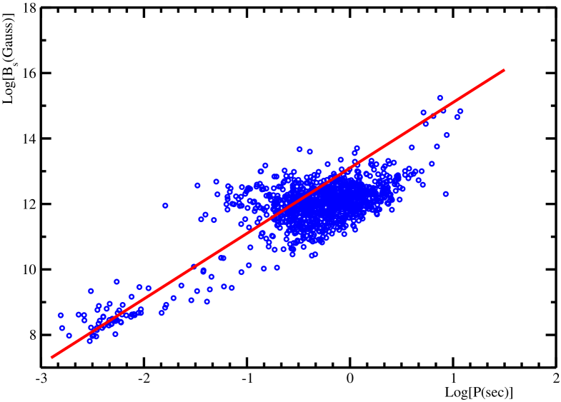
Figure 1: Inferred magnetic field $B_{S}$ plotted versus stellar period for 1194 pulsars taken from the ATNF Pulsar Catalog [49]. Full red line corresponds to Eq. (2.5) with $B_{1}\,\simeq\,1.3\,10^{13}\;Gauss$.

From previous equations it follows that $\mu_{d}\,>\mu_{u}\,>\,\mu_{e}$. Moreover, it turns out that the chemical potentials are monotonic decreasing smooth functions of the distance from the center of the star. In general, the quark chemical potentials $\mu_{d}$ and $\mu_{u}$ are smaller that the strength of the chromomagnetic condensate $\sqrt{gH}$. So that, up and down quarks occupy the lowest Landau levels. However, for certain values of the central energy density it happens that $\frac{\mu_{d}}{\sqrt{gH}}\,\gtrsim\,1$ in the stellar core. Thus, a fraction of down quarks must jump into higher Landau levels leading to a central core with energy density $\varepsilon_{c}$ somewhat greater than the energy density outside the core. Now, these quarks in the inner core produce a vector current in response to the chromomagnetic condensate. Obviously, the quark current tends to screen the chromomagnetic condensate by a very tiny amount. However, since the down quark has an electric charge $q_{d}=-\frac{1}{3}\,e$, the quark current generates in the core a uniform magnetic field parallel to the chromomagnetic condensate with strength:

$$B_{c}\;\;\simeq\;\;\frac{e}{96\,\pi}\;\;gH\;\;.$$ (2.4)

Outside the core the magnetic field is dipolar leading to surface magnetic field given by Eq. (1.3). In general the formation of the inner core denser than the outer core is contrasted by the centrifugal force produced by stellar rotation. Since the centrifugal force is proportional to the square of the stellar rotation frequency, this leads us to argue that the surface magnetic field strength is proportional to the square of the stellar period:

$$B_{S}\;\;\simeq\;\;B_{1}\;\left(\frac{P}{1\,sec}\right)^{2}\;\;\;\;,$$ (2.5)

where $B_{1}$ is the surface magnetic field for pulsars with nominal period $P\,=\,1\;sec$. Indeed, in Fig. 1 we we display the surface magnetic field strength $B_{S}$ inferred from (for instance, see Ref. [48]):

$$B_{S}\;\;\simeq\;\;3.1\;10^{19}\;\;\sqrt{P\;\dot{P}}\;Gauss\;\;,$$ (2.6)

versus the period. Remarkably, assuming $B_{1}\,\simeq\,1.3\,10^{13}\;Gauss$, we find the Eq. (2.5) accounts rather well the inferred magnetic field for pulsars ranging from millisecond pulsars up to anomalous $X$-ray pulsars and soft-gamma repeaters. As a consequence of Eq. (2.5), we see that the dipolar magnetic field is time dependent. In fact, it is easy to find:

$$B_{S}(t)\;\simeq\;B_{0}\;\;\left(1\;+\;2\;\frac{\dot{P}}{P}\;t\;\right)\;\;\;\;,$$ (2.7)

where $B_{0}$ indicates the magnetic field at the initial observation time. Note that Eq. (2.7) implies that the magnetic field varies on a time scale given by the characteristic age. Equation (2.7) leads to remarkable consequences discussed in Ref. [50]. Indeed, in Ref. [50], starting from Equation (2.7), we discussed a general mechanism which allows to explain naturally both radio and high energy emission from pulsars. We also discuss the plasma distribution in the region surrounding the pulsar, the pulsar wind and the formation of jet along the magnetic axis. We also suggested a plausible mechanism to generate pulsar proper motion velocities. In particular, in our emission mechanism there is a well defined geometric mapping between frequency and distance from the star which seems to be consistent with observations. In particular, in the recently detected binary radio pulsar system J0737-3039 [51, 52] it has been reported [53] the detection of features similar to drifting subpulses with a fluctuation frequency which is exactly the beat frequency between the period of the two pulsars. This direct influence of the electromagnetic radiation from one pulsar on the electromagnetic emission from the other pulsar can be naturally accounted for within our emission mechanism due to the geometric mapping between emission frequencies and distances. On the other hand, that effect cannot easily reconciled with the generally accepted model for pulsar radio emission which involves coherent radiation from very energetic $e^{+}-e^{-}$ pairs.
It is widely accepted that pulsar radio emission is powered by the rotational energy:

$$E_{R}\;=\;\frac{1}{2}\;I\;\;\omega^{2}\;\;\;,$$ (2.8)

so that, the spin-down power output is given by:

$$-\;\dot{E}_{R}\;=\;-\;I\;\;\omega\;\dot{\omega}\;\;=\;4\;\pi^{2}\;I\;\frac{\dot{P}}{P^{3}}\;.$$ (2.9)

On the other hand, an important source of energy is provided by the magnetic field. Indeed, the classical energy stored into the magnetic field is:

$$E_{B}\;=\;\frac{1}{8\,\pi}\;\int_{r\,\geq\,R}\;\;d^{3}r\;B^{2}(r)\;\;\;\;,$$ (2.10)

Assuming a dipolar magnetic field:

$$B(r)\;=\;B_{S}\;\;\left(\frac{R}{r}\right)^{3}\;\;for\;\;\;r\,\geq\,R\;\;\;\;,$$ (2.11)

Eq. (2.10) leads to:

$$E_{B}\;=\;\frac{1}{6}\;B_{S}^{2}\;\;R^{3}\;\;.$$ (2.12)

Now, from Eq. (2.7) the surface magnetic field is time dependent. So that, the magnetic power output is given by:

$$\dot{E}_{B}\;=\;\frac{2}{3}\;B_{0}^{2}\;\;R^{3}\;\;\;\frac{\dot{P}}{P}\;.$$ (2.13)

For rotation-powered pulsars it turns out that $\dot{E}_{B}\;\ll\;-\,\dot{E}_{R}$. However, if the dipolar magnetic field is strong enough, then the magnetic power Eq. (2.13) can be of the order, or even greater than the spin-down power. Thus, we may formulate a well defined criterion to distinguish rotation powered pulsars from magnetic powered pulsars. Indeed, until $\dot{E}_{B}\;<\;-\,\dot{E}_{R}$ there is enough rotation power to sustain the pulsar emission. On the other hand, when $\dot{E}_{B}\;\geq\;-\,\dot{E}_{R}$ all the rotation energy is stored into the increasing magnetic field and the pulsar emission is turned off. In fact, in the next Section we will derive the radio death line, which is the line that in the $P-\dot{P}$ plane separates rotation-powered pulsars from magnetic-powered pulsars. In the remainder of this Section, we discuss the recently detected radio pulsar with very strong surface magnetic field. We focus on the two radio pulsars with the strongest surface magnetic field: PSR J1718-3718 and PSR J1847-0130 . These pulsar have inferred surface magnetic fields well above the quantum critical field $B_{QED}$ above which some models [54] predict that radio emission should not occur. In particular, we have:

$$\begin{split}PSRJ1718-3718~{}\cite[cite]{[\@@bibref{}{Hobbs:2004}{}{}]}&\;\;\;\;\;\;\;P\;\simeq\;\;\;3.4\;\;sec\;\;,\;\;B_{S}\,\simeq\,7.4\;10^{13}\;Gauss\;\;,\\ PSRJ1847-0130~{}\cite[cite]{[\@@bibref{}{McLaughlin:2003}{}{}]}&\;\;\;\;\;\;\;P\;\simeq\;\;\;6.7\;\;sec\;\;,\;\;B_{S}\,\simeq\,9.4\;10^{13}\;Gauss\;\;.\end{split}$$ (2.14)

Both pulsars have average radio luminosities and surface magnetic fields larger than that of AXP 1E 2259+586. Now, using Eqs. (2.13), (2.9) , together with $I=\frac{2}{5}\,M\,R^{2}$, and Eq. (2.14) we get:

$$\begin{split}PSRJ1718-3718&\;\;\;\;-\;\dot{E}_{R}\;\simeq\;3.4\;10^{45}\;erg\;\;\;\frac{\dot{P}}{P}\;,\;\dot{E}_{B}\;\simeq\;4.7\;10^{44}\;erg\;\;\;\frac{\dot{P}}{P}\;\;,\\ PSRJ1847-0130&\;\;\;\;-\;\dot{E}_{R}\;\simeq\;8.8\;10^{44}\;erg\;\;\;\frac{\dot{P}}{P}\;,\;\dot{E}_{B}\;\simeq\;7.5\;10^{44}\;erg\;\;\;\frac{\dot{P}}{P}\;\;.\end{split}$$ (2.15)

We see that in any case: $\dot{E}_{B}\;<\;-\dot{E}_{R}$, so that there is enough rotational energy to power the pulsar emission.

3 RADIO DEATH LINE

As discussed in previous Section, until $\dot{E}_{B}\;<\;-\,\dot{E}_{R}$ the rotation power loss sustains the pulsar emission. We have already shown that this explain the otherwise puzzling pulsar activity for pulsars with inferred magnetic fields well above the critical field $B_{QED}$. Even more, the two pulsars PSR J1718-3718 and PSR J1847-0130 have magnetic fields which are well above the magnetic field of the anomalous $X$-ray pulsar AXP 1E 2259+586. Up to now, it was unclear how these high-field pulsars and anomalous $X$-ray pulsars can have such similar spin-down parameters but vastly different emission properties. We have offered a natural explanation for the pulsar activity for high-field radio pulsars. In this Section we explain why anomalous $X$-ray pulsars and soft gamma repeaters are radio quiet pulsars.

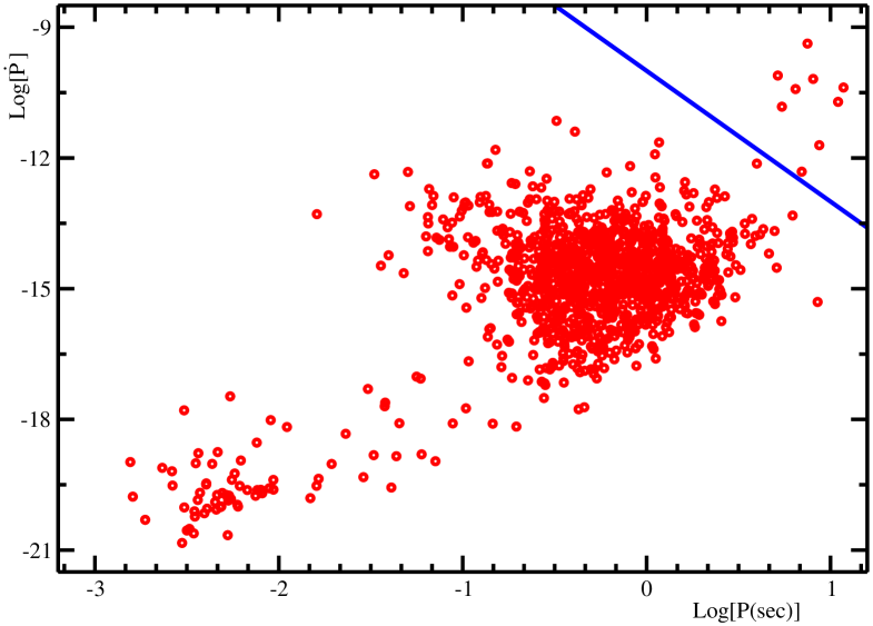
Figure 2: Period derivative plotted versus stellar period for 1194 pulsars taken from the ATNF Pulsar Catalog [49]. Full blue line corresponds to Eq. (3.4)

When $\dot{E}_{B}\;\geq\;-\,\dot{E}_{R}$ all the rotation energy is stored into the increasing magnetic field and the pulsar emission is turned off. As a consequence pulsars with strong enough magnetic fields are radio quiet. Accordingly we see that the condition:

$$\dot{E}_{B}\;=\;-\;\dot{E}_{R}\;\;.$$ (3.1)

is able to distinguish rotation powered pulsars from magnetic powered pulsars. Now, using [48]

$$B_{S}\;\simeq\;\sqrt{\frac{3\,I\,P\,\dot{P}}{8\,\pi^{2}\,R^{6}}}\;\;\;,$$ (3.2)

we recast Eq. (3.1) into:

$$P^{3}\,\dot{P}\;=\;16\,\pi^{4}\,R^{3}\;\;\;.$$ (3.3)

Using the canonical radius $R\simeq 10\,Km$, we get:

$$3\;\log(P)\,+\,\log(\dot{P})\;\simeq\;-\,10\;\;\;.$$ (3.4)

Equation (3.4) is a straight line, plotted in Fig. 2, in the $\log(P)-\log(\dot{P})$ plane. In Figure. 2 we have also displayed 1194 pulsars taken from the ATNF Pulsar Catalog [49]. We see that rotation powered pulsars, ranging from millisecond pulsars up to radio pulsars, do indeed lie below our Eq. (3.4). Note that in Fig. 2 the recently detected high magnetic field pulsars are not included. However, we have already argued in previous Section that these pulsars have spin parameters which indicate that these pulsars are rotation powered. On the other hand, Fig. 2 shows that all soft gamma-ray repeaters and anomalous $X$-ray pulsars in the ATNF Pulsar Catalog lie above our line Eq. (3.4). In particular, in Fig. 2 the pulsar above and nearest to the line Eq. (3.4) corresponds to AXP 1E 2259+586. So that, we see that our radio dead line, Eq. (3.4), correctly predicts that AXP 1E 2259+586 is not a radio pulsar even though the magnetic field is lower than that in radio pulsars PSR J1718-3718 and PSR J1847-0130. We may conclude that pulsars above our dead line are magnetars, i.e. magnetic powered pulsars. The emission properties of magnetars are quite different from rotation powered pulsars. The emission from magnetars consists in thermal blackbody radiation form the surface. In addition, it could eventually also be present a faint power-law emission superimposed to the thermal radiation. As discussed in Appendix, this soft faint emission is caused by the thermal radiation reprocessed in the magnetosphere. In Ref. [10] we suggested that RXJ 1856.5-3754 is exactly in this state. On the other hand, the energy stored into the magnetic field can be released if the star undergoes a glitch. Indeed, as thoroughly discussed in the next Section, glitches originate from dissipative effects in the inner core of the star leading to a decrease of the strength of the core magnetic field. So that, soon after the glitch there is a release of magnetic energy. We have already suggested in Ref. [10] that this picture is consistent with the long-term variability in the $X$-ray emission of RXJ 0720.4-3125. Remarkably, a recent timing analysis of the isolated pulsar RXJ 0720.4-3125 performed in Ref. [57] suggested that, among different possibilities, glitching may have occurred in this pulsar.

4 GLITCHES IN MAGNETARS

In p-stars there is a natural mechanism to generate a dipolar magnetic field, namely the generation of the dipolar magnetic field is enforced by the formation of a dense inner core composed mainly by down quarks. A quite straightforward calculation, which will be presented elsewhere, leads to the conclusion that down quarks in the inner core produce a vector current in response to the chromomagnetic condensate. This quark current, in turn, generates in the core a uniform magnetic field parallel to the chromomagnetic condensate with strength given by Eq. (2.4). Outside the core the magnetic field is dipolar. Now, we note that the inner core is characterized by huge conductivity, while outer core quarks are freezed into the lowest Landau levels. So that, due to the energy gap between the lowest Landau levels and the higher ones, the quarks outside the core cannot support any electrical current. As a consequence, the magnetic field in the region outside the core is not screened leading to our previous Eq. (1.3). For later convenience, after taking into account Eq. (2.4), we rewrite Eq. (1.3) as:

$$B_{S}\;\;\simeq\;\;B_{c}\;\;\left(\frac{R_{c}}{R}\right)^{3}\;\;,\;\;B_{c}\;\simeq\;\;\frac{e}{96\,\pi}\;\;gH\;\;.$$ (4.1)

In Figure 3 we display a schematic view of the interior of a p-star.

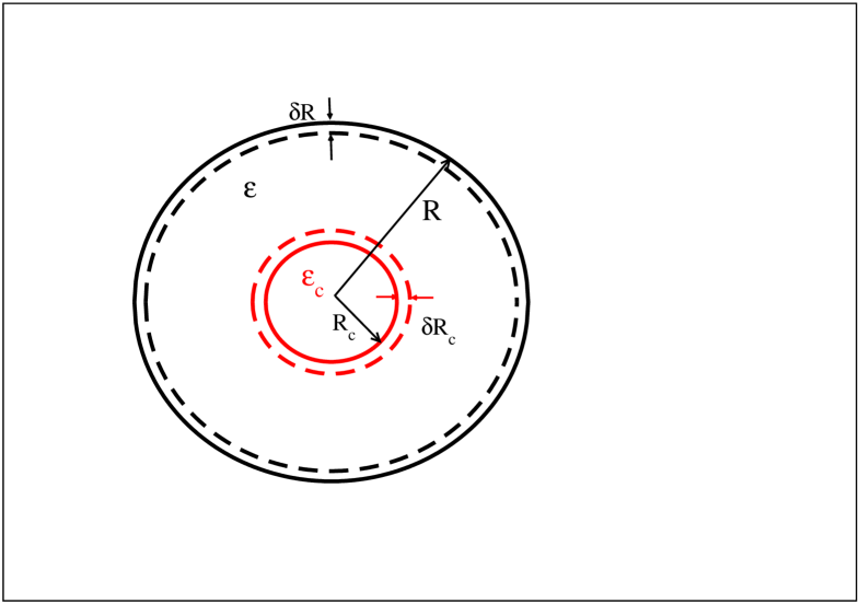
Figure 3: Schematic view of the interior of a p-star. $R_{c}$ and $R$ represent the inner core and stellar radii respectively; $\varepsilon_{c}$ is the energy density of the inner core, $\varepsilon$ is the energy density outside the core.

The presence of the inner core uniformly magnetized leads to well defined glitch mechanism in p-stars. Indeed, dissipative effects, which are more pronounced in young stars, tend to decrease the strength of the core magnetic field. On the other hand, when $B_{c}$ decreases due to dissipation effects, then the magnetic flux locally decreases and, according to Lenz’s law, induces a current which resists to the reduction of the magnetic flux. This means that some quarks must flow into the core by jumping onto higher Landau levels. In other words, the core radius must increase. Moreover, due to very high conductivity of quarks in the core, we have:

$$B_{c}\;\;R_{c}^{2}\simeq\;constant\;,$$ (4.2)

which implies:

$$\frac{\delta\,B_{c}}{B_{c}}\;+\;2\;\frac{\delta\,R_{c}}{R_{c}}\;\simeq\;0\;,$$ (4.3)

or

$$\frac{\delta\,R_{c}}{R_{c}}\;\simeq\;-\;\frac{1}{2}\;\frac{\delta\,B_{c}}{B_{c}}\;.$$ (4.4)

Equation (4.4) confirms that to the decrease of the core magnetic field, $\delta B_{c}<0$, it corresponds an increase of the inner core radius $\delta R_{c}>0$. This sudden variation of the radius of the inner core leads to glitches. Indeed, it is straightforward to show that the magnetic moment:

$$\emph{m}\;=\;B_{S}\;R^{3}\;=\;\;B_{c}\;R_{c}^{3}\;$$ (4.5)

where we used Eq. (4.1), must increase in the glitch. Using Eq. (4.4), we get:

$$\frac{\delta\,\emph{m}}{\emph{m}}\;=\;\frac{\delta\,B_{c}}{B_{c}}\;+\;3\;\frac{\delta\,R_{c}}{R_{c}}\;\simeq\;\frac{\delta\,R_{c}}{R_{c}}\;>\;0\;,$$ (4.6)

Another interesting consequence of the glitch is that the stellar radius $R$ must decrease, i.e. the star contracts. This is an inevitable consequence of the increase of the inner core, which is characterized by an energy density $\varepsilon_{c}$ higher then the outer core density $\varepsilon$. As a consequence the variation of radius is negative: $\delta R<0$ (see Fig. 3 ). In radio pulsar, where the magnetic energy can be neglected, conservation of the mass leads to:

$$\frac{\delta\,R}{R}\;\simeq\;-\;\frac{\varepsilon_{c}-\varepsilon}{\overline{\varepsilon}}\;\left(\frac{R_{c}}{R}\right)^{3}\;\frac{\delta\,R_{c}}{R_{c}}\;,$$ (4.7)

where $\overline{\varepsilon}$ is the average energy density. In general, we may assume that $\frac{\varepsilon_{c}-\varepsilon}{\overline{\varepsilon}}$ is a constant of order unity. So that Eq. (4.7) becomes:

$$\frac{\delta\,R}{R}\;\simeq\;-\;\left(\frac{R_{c}}{R}\right)^{3}\;\frac{\delta\,R_{c}}{R_{c}}\;.$$ (4.8)

Note that the ratio $\left(\frac{R_{c}}{R}\right)^{3}$ can be estimate from Eq. (4.1) once the surface magnetic field is known. We find that, even for magnetars, $\left(\frac{R_{c}}{R}\right)^{3}$ is of order $10^{-2}$ or less. So that our Eqs. (4.1) and (4.8) show that:

$$\delta R\;<\;0\;\;\;,\;\;\;-\;\frac{\delta\,R}{R}\;\ll\;\frac{\delta\,R_{c}}{R_{c}}\;\;.$$ (4.9)

As is well known, because the external magnetic braking torque, pulsars slow down according to (e.g. see Ref. [48]):

$$-\;\dot{\nu}\;\propto\;\emph{m}^{2}\;I^{-1}\;\nu^{3}\;.$$ (4.10)

So that:

$$\frac{\delta\dot{\nu}}{\dot{\nu}}\;=\;2\;\frac{\delta\emph{m}}{\emph{m}}\;-\;\frac{\delta I}{I}\;+\;3\;\frac{\delta\nu}{\nu}\;\;.$$ (4.11)

From conservation of angular momentum we have:

$$|\frac{\delta I}{I}|\;\;\simeq\;\;|\frac{\delta\nu}{\nu}|\;\;.$$ (4.12)

Moreover, from observational data it turns out that:

$$|\frac{\delta\dot{\nu}}{\dot{\nu}}|\;\;\gg\;\;|\frac{\delta\nu}{\nu}|\;\;,$$ (4.13)

so that Eq. (4.11) becomes:

$$\frac{\delta\dot{\nu}}{\dot{\nu}}\;\simeq\;2\;\frac{\delta\emph{m}}{\emph{m}}\;\simeq\;2\;\frac{\delta\,R_{c}}{R_{c}}\;\simeq\;-\;\frac{\delta\,B_{c}}{B_{c}}\;\;,$$ (4.14)

where we used Eqs. (4.6) and (4.4). Equation (4.14) does show that the variation of the radius of the inner core leads to a glitch.
In rotation powered pulsar, starting from Eq. (4.7) one can show that $|\frac{\delta\nu}{\nu}|\simeq|\frac{\delta\,R}{R}|$. So that, taking into account Eq. (4.9) we recover the phenomenological relation Eq. (4.13). A full account of glitches in radio pulsar will be presented elsewhere. Glitches in magnetars are considered in the next Section, where we show that, indeed, Eqs. (4.9) and (4.13) hold even in magnetars.
The most dramatic effect induced by glitches in magnetars is the release of a huge amount of magnetic energy in the interior of the star and into the magnetosphere. To see this, let us consider the energy stored into the magnetic field in the interior of the magnetar. We have:

$$E_{B}^{\emph{int}}\;=\;\frac{1}{6}\;R_{c}^{3}\;B_{c}^{2}\;+\;\frac{1}{8\,\pi}\;\int_{R_{c}}^{R}\;\;d^{3}r\;\left[B_{c}\;\left(\frac{R_{c}}{r}\right)^{3}\right]^{2}\;\;\;,$$ (4.15)

where the first term is the energy stored into the core where the magnetic field is uniform. The variation of the magnetic energy Eq. (4.15) caused by a glitch is easily evaluated. Taking into account Eq. (4.4) and $\left(\frac{R_{c}}{R}\right)^{3}\ll 1$, we get:

$$\delta\,E_{B}^{\emph{int}}\;\simeq\;-\;\frac{1}{3}\;R^{3}\;B_{S}^{2}\;\left(\frac{R}{R_{c}}\right)^{3}\;\frac{\delta R_{c}}{R_{c}}\;-\;\frac{1}{2}\;R^{3}\;B_{S}^{2}\;\frac{\delta R_{c}}{R_{c}}\;\simeq\;-\;\frac{1}{3}\;R^{3}\;B_{S}^{2}\;\left(\frac{R}{R_{c}}\right)^{3}\;\frac{\delta R_{c}}{R_{c}}\;.$$ (4.16)

Equation (4.16) shows that there is a decrease of the magnetic energy. So that after a glitch in magnetars a huge magnetic energy is released in the interior of the star. We shall see that this energy is enough to sustain the quiescent emission. On the other hand, the glitch induces also a sudden variation of the magnetic energy stored into the magnetosphere. Indeed, from Eq. (4.1) we find:

$$\frac{\delta B_{S}}{B_{S}}\;=\;\frac{\delta B_{c}}{B_{c}}\;+\;3\;\frac{\delta R_{c}}{R_{c}}\;-\;3\;\frac{\delta R}{R}\;\simeq\;\frac{\delta R_{c}}{R_{c}}\;-\;3\;\frac{\delta R}{R}\;\simeq\;\frac{\delta R_{c}}{R_{c}}\;>\;0\;\;.$$ (4.17)

Thus, the magnetic energy stored into the magnetosphere:

$$E_{B}^{\emph{ext}}\;=\;\frac{1}{8\,\pi}\;\int_{R}^{\infty}\;\;d^{3}r\;\left[B_{S}\;\left(\frac{R}{r}\right)^{3}\right]^{2}\;=\;\frac{1}{6}\;B_{S}^{2}\;\;R^{3}\;\;,$$ (4.18)

increases by:

$$\delta E_{B}^{\emph{ext}}\;=\;\frac{1}{3}\;R^{3}\;B_{S}^{2}\;\left(\frac{\delta B_{S}}{B_{S}}\;+\;\frac{3}{2}\frac{\delta R}{R}\right)\;\simeq\;\frac{1}{3}\;R^{3}\;B_{S}^{2}\;\frac{\delta B_{S}}{B_{S}}\;>\;0\;\;.$$ (4.19)

This magnetic energy is directly injected into the magnetosphere, where it is dissipated by well defined physical mechanism discussed in Section 4.3, and it is responsible for bursts in soft gamma-ray repeaters and anomalous $X$-ray pulsars.
To summarize, in this Section we have found that dissipative phenomena in the inner core of a p-star tend to decrease the strength of the core magnetic field. This, in turn, results in an increase of the radius of the core $\delta R_{c}>0$, and in a contraction of the surface of the star, $\delta R<0$. We have also show that the glitch releases an amount of magnetic energy in the interior of the star and injects magnetic energy into the magnetosphere, where it is completely dissipated. Below we will show that these magnetic glitches are responsible for the quiescent emission and bursts in gamma-ray repeaters and anomalous $X$-ray pulsars. Interestingly enough, in Ref. [58] it was shown that SGR events and earthquakes share several distinctive statistical properties, namely: power-law energy distributions, log-symmetric waiting time distributions, strong correlations between waiting times of successive events, and weak correlations between waiting times and intensities. These statistical properties of bursts can be easily understood if bursts originate by the release of a small amount of energy from a reservoir of stored energy. As a matter of fact, in our theory the burst activity is accounted for by the release of a tiny fraction of magnetic energy stored in magnetars. Even for giant bursts we find that the released energy is a few per cent of the magnetic energy. Moreover, the authors of Ref. [59] noticed that there is a significantly statistical similarity between the bursts from SGR 1806-20 and the microglitches observed from the Vela pulsar with $|\frac{\delta\nu}{\nu}|\thicksim 10^{-9}$. So that we see that these early statistical studies of bursts are in complete agreement with our theory for bursts in magnetars. Even more, we shall show that after a giant glitch there is an intense burst activity quite similar to the settling earthquakes following a strong earthquake.

4.1 BRAKING GLITCHES

In Section 4 we found that magnetic glitches in p-stars lead to:

$$\frac{\delta\dot{\nu}}{\dot{\nu}}\;\;\simeq\;\;-\;\frac{\delta B_{c}}{B_{c}}\;>\;0\;\;.$$ (4.20)

Since there is variation of both the inner core and the stellar radius, the moment of inertia of the star undergoes a variation of $\delta I$. It is easy to see that the increase of the inner core leads to an increase of the moment of inertia $I$; on the other hand, the reduction of the stellar radius implies $\delta I<0$. In radio pulsar, where, by neglecting the variation of the magnetic energy, the conservation of the mass leads to Eq. (4.8), one can show that:

$$\frac{\delta I}{I}\;\;\simeq\;\;\frac{\delta R}{R}\;<\;0\;\;.$$ (4.21)

Moreover, from conservation of angular momentum:

$$\frac{\delta I}{I}\;\;=\;-\;\frac{\delta\nu}{\nu}\;\;,$$ (4.22)

it follows:

$$0\;<\;\;\frac{\delta\nu}{\nu}\;\;\simeq\;\;-\;\frac{\delta R}{R}\;\ll\;-\;\frac{\delta B_{c}}{B_{c}}\;\;\simeq\;\;\frac{\delta\dot{\nu}}{\dot{\nu}}\;\;.$$ (4.23)

For magnetars, namely p-stars with super strong magnetic field, the variation of magnetic energy cannot be longer neglected. In this case, since the magnetic energy decreases, we have that the surface contraction in magnetars is smaller than in radio pulsars. That means that Eq. (4.9) holds even for magnetars. Moreover, since in radio pulsars we known that:

$$\frac{\delta\nu}{\nu}\;\;=\;-\;\frac{\delta I}{I}\;\simeq\;\;-\;\frac{\delta R}{R}\;\lesssim\;10^{-6}\;\;,$$ (4.24)

we see that in magnetars the following bound must hold:

$$-\;\frac{\delta R}{R}\;\lesssim\;10^{-6}\;\;.$$ (4.25)

As a consequence we may write:

$$\frac{\delta I}{I}\;\;=\;\;\left(\frac{\delta I}{I}\right)_{core}\;\;+\;\;\left(\frac{\delta I}{I}\right)_{surf}\;\;,\;\;\left(\frac{\delta I}{I}\right)_{surf}\simeq\;\;\frac{\delta R}{R}\;<\;0\;.$$ (4.26)

As we show in a moment, the variation of the moment of inertia induced by the core is positive. So that if the core contribution overcomes the surface contribution to $\delta I$ we have a braking glitch where $-\frac{\delta\nu}{\nu}=\frac{\delta P}{P}>0$.
We believe that the most compelling evidence in support to our proposal comes from the anomalous $X$-ray pulsar AXP 1E 2259+586. As reported in Ref. [60], the timing data showed that a large glitch occurred in AXP 1E 2259+586 coincident with the 2002 June giant burst. Remarkably, at the time of the giant flare on 1998 August 27, the soft gamma ray repeater SGR 1900+14 displayed a discontinuous spin-down consistent with a braking glitch [61]. Our theory is able to explain why AXP 1E 2259+586 displayed a normal glitch, while SGR 1900+14 suffered a braking glitch. To see this, we recall the spin-down parameters of these pulsars:

$$\begin{split}\emph{SGR 1900+14}&\;\;\;P\;\simeq\;5.16\;sec\;,\;\dot{P}\;\simeq\;1.1\;10^{-10}\;,\;B_{S}\;\simeq\;7.4\;10^{14}\;Gauss\;\;,\\ \emph{AXP 1E 2259+586}&\;\;\;P\;\simeq\;6.98\;sec\;,\;\dot{P}\;\simeq\;2.0\;10^{-14}\;,\;B_{S}\;\simeq\;1.2\;10^{13}\;Gauss\;\;.\end{split}$$ (4.27)

For canonical magnetars with $M\,\simeq 1.4\,M_{\bigodot}$ and radius $R\,\simeq 10\,Km$, we have $\sqrt{gH}\simeq 0.55\;GeV$. So that, using $1\,GeV^{2}\,\simeq\,5.12\,10^{19}\,Gauss$, we rewrite Eq. (4.1) as:

$$B_{S}\;\;\simeq\;\;1.54\;10^{16}\;\left(\frac{R_{c}}{R}\right)^{3}\;\;Gauss\;\;.$$ (4.28)

Combining Eqs. (4.27) and (4.28) we get:

$$\begin{split}\emph{SGR 1900+14}&\;\;\;\;\;\;\;\;\left(\frac{R_{c}}{R}\right)^{3}\;\;\simeq\;4.81\;10^{-2}\;\;,\\ \emph{AXP 1E 2259+586}&\;\;\;\;\;\;\;\;\left(\frac{R_{c}}{R}\right)^{3}\;\;\simeq\;0.78\;10^{-3}\;\;.\end{split}$$ (4.29)

According to Eqs. (4.20),  (4.22) and (4.26), to evaluate the sudden variation of the frequency and frequency derivative, we need $\delta R$ and $\delta R_{c}$. These parameters can be estimate from the energy released during the giant bursts. In the case of AXP 1E 2259+586, the giant 2002 June burst followed an intense burst activity which lasted for about one year. The authors of Ref. [60], assuming a distance of $3\;kpc$ to 1E 2259+586, measured an energy release of $2.7\,10^{39}\,ergs$ and $2.1\,10^{41}\,ergs$ for the fast and slow decay intervals, respectively. Due to this uncertainty, we conservatively estimate the energy released during the giant burst to be:

$$\emph{AXP 1E 2259+586}\;\;\;\;\;E_{\emph{burst}}\;\;\;\;\simeq\;1.0\;10^{40}\;\;ergs\;\;.$$ (4.30)

On 1998 August 27, a giant burst from the soft gamma ray repeater SGR 1900+14 was recorded. The estimate energy released was:

$$\emph{SGR 1900+14}\;\;\;\;\;E_{\emph{burst}}\;\;\;\;\simeq\;1.0\;10^{44}\;\;ergs\;\;.$$ (4.31)

As we have already discussed in Sect. 4, the energy released during a burst in magnetars is given by the magnetic energy directly injected and dissipated into the magnetosphere, Eq. (4.19). We rewrite Eq. (4.19) as

$$\delta E_{B}^{\emph{ext}}\;\simeq\;\frac{1}{3}\;R^{3}\;B_{S}^{2}\;\frac{\delta B_{S}}{B_{S}}\;\simeq\;2.6\;10^{44}\;ergs\;\left(\frac{B_{S}}{10^{14}\,Gauss}\right)^{2}\;\frac{\delta B_{S}}{B_{S}}\;\;.$$ (4.32)

So that, combining Eqs. (4.32), (4.31), (4.30) and (4.27) we get:

$$\begin{split}\emph{SGR 1900+14}&\;\;\;\;\;\;\;\;\frac{\delta B_{S}}{B_{S}}\;\simeq\;\frac{\delta R_{c}}{R_{c}}\;\simeq\;0.70\;10^{-2}\;\;\;,\\ \emph{AXP 1E 2259+586}&\;\;\;\;\;\;\;\;\frac{\delta B_{S}}{B_{S}}\;\simeq\;\frac{\delta R_{c}}{R_{c}}\;\simeq\;0.27\;10^{-2}\;\;\;.\end{split}$$ (4.33)

Thus, according to Eq. (4.20) we may estimate the sudden variation of $\dot{\nu}$:

$$\frac{\delta\dot{\nu}}{\dot{\nu}}\;\;\simeq\;\;2\;\frac{\delta\,R_{c}}{R_{c}}\;\;\thicksim\;\;10^{-2}\;\;,$$ (4.34)

for both glitches. On the other hand we have:

$$\left(\frac{\delta I}{I}\right)_{core}\;\;\simeq\;\;\frac{15}{2}\;\frac{\varepsilon_{c}-\varepsilon}{\overline{\varepsilon}}\;\left(\frac{R_{c}}{R}\right)^{5}\;\frac{\delta\,R_{c}}{R_{c}}\;\;\simeq\;\;\frac{15}{2}\;\;\left(\frac{R_{c}}{R}\right)^{5}\;\frac{\delta\,R_{c}}{R_{c}}\;\;,$$ (4.35)

leading to:

$$\begin{split}\emph{SGR 1900+14}&\;\;\;\;\;\;\;\;\left(\frac{\delta I}{I}\right)_{core}\simeq\;3.34\;\;10^{-4}\;\;\;,\\ \emph{AXP 1E 2259+586}&\;\;\;\;\;\;\;\;\left(\frac{\delta I}{I}\right)_{core}\simeq\;1.34\;\;10^{-7}\;\;\;.\end{split}$$ (4.36)

On the other hand, we expect that during the giant glitch $\left(\frac{\delta I}{I}\right)_{surf}\thicksim 10^{-6}$. As a consequence, for AXP 1E 2259+586 the core contribution is negligible with respect to the surface contribution to $\delta I$. In other words, AXP 1E 2259+586 displays a normal glitch with $\frac{\delta\nu}{\nu}\thicksim 10^{-6}$. On the contrary, Eq. (4.36) indicates that SGR 1900+14 suffered a braking glitch with $\frac{\delta\nu}{\nu}\thicksim-3.34\;10^{-4}$ giving:

$$\Delta\;P\;\;\simeq\;\;1.72\;\;10^{-3}\;\;sec\;\;.$$ (4.37)

We would like to stress that our theory is in remarkable agreement with observations, for a glitch of size $\frac{\delta\nu}{\nu}=4.24(11)\;10^{-6}$ was observed in AXP 1E 2259+586 which preceded the burst activity [60]. Moreover, our theory predicts a sudden increase of the spin-down torque according to Eq. (4.34). In Ref. [60] it is pointed out that it was not possible to give a reliable estimate of the variation of the frequency derivative since the pulse profile was undergoing large changes, thus compromising the phase alignment with the pulse profile template. Indeed, as discussed in Sect. 5.1, soon after the giant burst AXP 1E 2259+586 suffered an intense burst activity. Now, according to our theory, during the burst activity there is both a continuous injection of magnetic energy into the magnetosphere and variation of the magnetic torque explaining the anomalous timing noise observed in 1E 2259+586. In addition, the authors of Ref. [61] reported a gradual increase of the nominal spin-down rate and a discontinuous spin down event associated with the 1998 August 27 flare from SGR 1900+14. Extrapolating the long-term trends found before and after August 27, they found evidence of a braking glitch with $\Delta P\,\simeq\,0.57(2)\;10^{-3}\;sec$. In view of our theoretical uncertainties, the agreement with our Eq. (4.37) is rather good.
We feel that it is worthwhile to point out that the standard magnetar theory is completely unable to predict the remarkable evidence of braking glitches. As a matter of fact, to our knowledge, the only attempt to explain the braking glitch observed in SGR 1900+14 is done in Ref. [62] where it is suggested that violent August 27 event involved a glitch. However, the magnitude of the glitch was estimated by scaling to the largest glitches in young, active pulsars with similar spin-down ages and internal temperature. In this way they deduced the estimate $|\frac{\Delta P}{P}|\thicksim 10^{-5}$ to $10^{-4}$. In our opinion, this can hardly be considered a valid explanation for the braking glitch. First, the authors of Ref. [62] overlooked the well known fact that radio pulsars display normal glitches and no braking glitches. Second, these authors cannot explain why AXP 1E 2259+586 displayed a normal glitch instead of a braking glitch.
Let us conclude this Section by briefly discussing the 2004 December 27 giant flare from SGR 1806-20. During this tremendous outburst SGR 1806-20 released a huge amount of energy, $E_{\emph{burst}}\thicksim 10^{46}\;ergs$. Using the spin-down parameters reported in Ref.  [63]:

$$\emph{SGR 1806-20}\;\;\;P\;\simeq\;7.55\;sec\;,\;\dot{P}\;\simeq\;5.5\;10^{-10}\;,\;B_{S}\;\simeq\;2.0\;10^{15}\;Gauss\;\;,$$ (4.38)

we find:

$$\emph{SGR 1806-20}\;\;\;\;\;\frac{\delta B_{S}}{B_{S}}\;\simeq\;\frac{\delta R_{c}}{R_{c}}\;\simeq\;9.6\;10^{-2}\;\;.$$ (4.39)

Thus, we predict that SGR 1806-20 should display a gigantic braking glitch with $\frac{\Delta P}{P}\simeq 2.4\;10^{-2}$, or :

$$\Delta\;P\;\;\simeq\;\;1.8\;\;10^{-1}\;\;sec\;\;.$$ (4.40)

4.2 QUIESCENT LUMINOSITY

The basic mechanism to explain the quiescent $X$-ray emission in our magnetars is the internal dissipation of magnetic energy. Our mechanism is basically the same as in the standard magnetar model based on neutron star [45]. Below we shall critically compare our proposal with the standard theory.
In Section 4 we showed that during a glitch there is a huge amount of magnetic energy released into the magnetar:

$$-\;\delta\,E_{B}^{\emph{int}}\;\;\simeq\;\;\frac{1}{3}\;R^{3}\;B_{S}^{2}\;\left(\frac{R}{R_{c}}\right)^{3}\;\frac{\delta R_{c}}{R_{c}}\;.$$ (4.41)

As in previous Section, we use SGR 1900+14 and AXP 1E 2259+586 as prototypes for soft gamma ray repeaters and anomalous $X$-ray pulsars, respectively. Using the results of Sect. 4.1, we find:

$$\begin{split}\emph{SGR 1900+14}&\;\;\;\;\;\;\;\;-\;\delta\,E_{B}^{\emph{int}}\;\;\simeq\;\;3.0\;\;10^{47}\;\;erg\;\;\frac{\delta R_{c}}{R_{c}}\;\;,\\ \emph{AXP 1E 2259+586}&\;\;\;\;\;\;\;\;-\;\delta\,E_{B}^{\emph{int}}\;\;\simeq\;\;4.8\;\;10^{45}\;\;erg\;\;\frac{\delta R_{c}}{R_{c}}\;\;.\end{split}$$ (4.42)

This release of magnetic energy is dissipated leading to observable surface luminosity. To see this, we need a thermal evolution model which calculates the interior temperature distribution. In the case of neutron stars such a calculation has been performed in Ref. [64], where it is showed that the isothermal approximation is a rather good approximation in the range of inner temperatures of interest. The equation which determines the thermal history of a p-star has been discussed in Ref. [9] in the isothermal approximation:

$$C_{V}\;\frac{dT}{dt}\;=\;-\;(L_{\nu}\;+\;L_{\gamma})\;,$$ (4.43)

where $L_{\nu}$ is the neutrino luminosity, $L_{\gamma}$ is the photon luminosity and $C_{V}$ is the specific heat. Assuming blackbody photon emission from the surface at an effective surface temperature $T_{S}$ we have:

$$L_{\gamma}\;=\;4\,\pi\,R^{2}\,\sigma_{SB}\,T_{S}^{4}\;,$$ (4.44)

where $\sigma_{SB}$ is the $Stefan-Boltzmann$ constant. In Ref. [9] we assumed that the surface and interior temperature were related by:

$$\frac{T_{S}}{T}\;=\;10^{-2}\;a\;\;.$$ (4.45)

Equation (4.45) is relevant for a p-star which is not bare, namely for p-stars which are endowed with a thin crust. It turns out [10] that p-stars have a sharp edge of thickness of the order of about $1\;fermi$. On the other hand, electrons which are bound by the coulomb attraction, extend several hundred fermis beyond the edge. As a consequence, on the surface of the star there is a positively charged layer which is able to support a thin crust of ordinary matter. The vacuum gap between the core and the crust, which is of order of several hundred fermis, leads to a strong suppression of the surface temperature with respect to the core temperature. The precise relation between $T_{S}$ and $T$ could be obtained by a careful study of the crust and core thermal interaction. In any case, our phenomenological relation Eq. (4.45) allows a wide variation of $T_{S}$, which encompasses the neutron star relation (see, for instance, Ref. [65]). Moreover, our cooling curves display a rather weak dependence on the parameter $a$ in Eq. (4.45). Since we are interested in the quiescent luminosity, we do not need to known the precise value of this parameter. So that, in the following we shall assume $a\thicksim 1$. In other words, we assume:

$$T_{S}\;\;\simeq\;\;10^{-2}\;\;T\;\;\;.$$ (4.46)

Obviously, the parameter $a$ is relevant to evaluate the surface temperature once the core temperature is given. Note that, in the relevant range of core temperature $T\thicksim 10^{8}$ $\,{}^{\circ}K$, our Eq. (4.46) is practically identical to the parametrization adopted in Ref. [45] within the standard magnetar model:

$$T_{S}\;\;\simeq\;\;1.3\;\;10^{6}\;{}^{\circ}K\;\;\left(\frac{T}{10^{8}\,{}^{\circ}K}\right)^{\frac{5}{9}}\;\;\;.$$ (4.47)

The neutrino luminosity $L_{\nu}$ in Eq. (4.43) is given by the direct $\beta$-decay quark reactions, the dominant cooling processes by neutrino emission. From the results of Ref. [9], we find:

$$L_{\nu}\;\;\simeq\;\;1.22\;\;10^{36}\;\;\frac{erg}{s}\;\;T_{9}^{8}\;\;\;,$$ (4.48)

where $T_{9}$ is the temperature in units of $10^{9}$ $\,{}^{\circ}K$. Note that the neutrino luminosity $L_{\nu}$ has the same temperature dependence as the neutrino luminosity by modified URCA reactions in neutron stars (see, for instance Ref. [30]), but it is more than two order of magnitude smaller. From the cooling curves reported in Ref. [9] we infer that the surface and interior temperature are almost constant up to time $\tau\thicksim 10^{5}\,years$. Observing that magnetars candidates are rather young pulsar with $\tau_{age}\lesssim 10^{5}\,years$, we may estimate the average surface luminosities as:

$$L_{\gamma}\;\;\simeq\;\frac{-\;\delta\,E_{B}^{\emph{int}}}{\tau_{age}}\;\;\;\;\;.$$ (4.49)

We assume $\tau_{age}\thickapprox\tau_{c}$ for SGR 1900+14. On the other hand, as discussed in Section 1, we known that for AXP 1E 2259+586 $\;\;\tau_{age}\thicksim 10^{3}\,years\ll\tau_{c}$. We get:

$$\begin{split}\emph{SGR 1900+14}&\;\;\;\;\;\;\;\;L_{\gamma}\;\;\simeq\;\;1.3\;\;10^{37}\;\;\frac{erg}{s}\;\;\frac{\delta R_{c}}{R_{c}}\;\;,\\ \emph{AXP 1E 2259+586}&\;\;\;\;\;\;\;\;L_{\gamma}\;\;\simeq\;\;1.5\;\;10^{35}\;\;\frac{erg}{s}\;\;\frac{\delta R_{c}}{R_{c}}\;\;.\end{split}$$ (4.50)

So that it is enough to assume that SGR 1900+14 suffered in the past a glitch with $\frac{\delta R_{c}}{R_{c}}\thicksim 10^{-2}$ to sustain the observed luminosity $L_{\gamma}\thicksim 10^{35}\;\frac{erg}{s}$ (assuming a distance of about $10\;kpc$). In the case of AXP 1E 2259+586, assuming a distance of about $3\;kpc$, the observed luminosity is $L_{\gamma}\thicksim 10^{34}\;\frac{erg}{s}$, so that we infer that this pulsar had suffered in the past a giant glitch with $\frac{\delta R_{c}}{R_{c}}\thicksim 10^{-1}$, quite similar to the recent SGR 1806-20 glitch.
Let us discuss the range of validity of our approximation. Equation (4.49) is valid as long as $L_{\gamma}$ dominates over $L_{\nu}$, otherwise the star is efficiently cooled by neutrino emission and the surface luminosity saturates to $L_{\gamma}^{max}$. We may quite easily evaluate this limiting luminosity from $L_{\gamma}^{max}\simeq L_{\nu}$. Using Eq. (4.46) and $R\simeq 10\;Km$, we get:

$$L_{\gamma}^{max}\;\;\simeq\;\;4.2\;\;10^{37}\;\frac{erg}{s}\;\;\;\;.$$ (4.51)

Note that, since our neutrino luminosity is reduced by more than two order of magnitude with respect to neutron stars, $L_{\gamma}^{max}$ is about two order of magnitude greater than the maximum allowed surface luminosity in neutron stars [64]. Thus, while our theory allows to account for observed luminosities up to $10^{36}\;\frac{erg}{s}$, the standard model based on neutron stars is in embarrassing contradiction with observations.
Let us, finally, comment on the quiescent thermal spectrum in our theory. As already discussed, the origin of the quiescent emission is the huge release of magnetic energy in the interior of the magnetar. Our previous estimate of the quiescent luminosities assumed that the interior temperature distribution was uniform. However, due to the huge magnetic field, the thermal conductivity is enhanced along the magnetic field. This comes out to be the case for both electron and quarks, since we argued that the magnetic and chromomagnetic fields are aligned . As a consequence, we expect that the quiescent spectrum should be parameterized as two blackbodies with parameter $R_{1}\,,\,T_{1}$ and $R_{2}\,,\,T_{2}$, respectively. Since the blackbody luminosities $L_{\gamma 1}$ and $L_{\gamma 2}$ are naturally of the same order, our previous estimates for the quiescent luminosities are unaffected. Moreover, since the thermal conductivity is enhanced along the magnetic field, the high temperature blackbody, with temperature $T_{2}$, originates from the heated polar magnetic cups. Thus we have:

$$\begin{split}&R_{1}\;\;\lesssim\;\;R\;\;\;,\;\;\;R_{2}\lesssim\;1\;Km\;\;,\;\;\\ &T_{2}\;\;>\;\;T_{1}\;\;\;,\;\;R_{1}\;\;>\;\;R_{2}\;\;,\;\;L_{\gamma 1}\;\;\simeq\;\;L_{\gamma 2}\;\;.\end{split}$$ (4.52)

Note that there is a natural anticorrelation between blackbody radii and temperatures. Customary, the quiescent spectrum of anomalous $X$-ray pulsars and soft gamma ray repeaters is fitted in terms of blackbody plus power law. In particular, it is assumed that the power law component extends to energy greater than an arbitrary cutoff energy $E_{cutoff}\simeq 2\,KeV$. It is worthwhile to stress that these parameterizations of the quiescent spectra are in essence phenomenological fits, for there are not sound physical motivations. Indeed, within the standard magnetar model [45] the power law should be related to hydromagnetic wind accelerated by Alfven waves. However, any physical justification for the arbitrary cutoff energy $E_{cutoff}$ is lacking. Moreover, the luminosity of the wind emission should increase with magnetic field strength as $L_{wind}\simeq L_{PL}\thicksim B_{S}^{2}$. On the other hand, the blackbody luminosities should scale as $B_{S}^{4.4}$ [45]. So that the ratio $L_{PL}/L_{BB}$ decreases with increasing magnetic field strengths, contrary to observations [66]. Finally, observations of a small energy dependence of pulsed fraction in some anomalous $X$-ray pulsars requires ad hoc tuning of the blackbody and power law components. Thus, we see that the standard magnetar model is in striking contradictions with observations.
On the contrary, in our theory well defined physical arguments lead to the two blackbody representation of the quiescent spectra, whose parameters are constrained by our Eq. (4.52). As a matter of fact, we have checked in literature that the quiescent spectra of both anomalous $X$-ray pulsars and soft gamma ray repeaters could be accounted for by two balckbodies. For instance, in Ref. [67] the quiescent spectrum of AXP 1E 1841-045 is well fitted with the standard power law plus blackbody (reduced $\chi^{2}/dof\simeq 1.11$), nevertheless the two blackbody model gives also a rather good fit (reduced $\chi^{2}/dof\simeq 1.12$). Interestingly enough the blackbody parameters:

$$\begin{split}&R_{1}\;=\;5.7\;\;^{+0.6}_{-0.5}\;\;\;\;Km\;\;\;,\;\;\;T_{1}\;=\;0.47\;\pm\;0.02\;\;KeV\;\;\;,\\ &R_{2}\;=\;0.36\;^{+0.08}_{-0.07}\;\;Km\;\;\;,\;\;\;T_{2}\;=\;1.5\;^{+0.2}_{-0.1}\;\;KeV\;\;\;,\end{split}$$ (4.53)

are in agreement with Eq. (4.52). Moreover, assuming that the power law component in the standard parametrization of quiescent spectra account for the hot blackbody component in our parametrization, we find that the suggestion $L_{\gamma 1}\;\simeq\;L_{\gamma 2}$ in Eq. (4.52) is in agreement with observations [66]. It should be stressed, however, that the two blackbodies are not the whole story. In Appendix we show that thermal photons originating from the hot polar cups are reprocessed by electrons trapped above the polar cups. These electrons, which are responsible for the faint low energy spectrum, could result in broad spectral features in the quiescent spectrum. These spectral features, in turn, could result in observable deviations from the two blackbody fit.
Another interesting consequence of the anisotropic distribution of the surface temperature due to strong magnetic fields is that the thermal surface blackbody radiation will be modulated by the stellar rotation. As a matter of fact, in Ref. [68] it is argued that the observed properties of anomalous $X$-ray pulsars can be accounted for by magnetars with a single hot region. It is remarkable that our interpretation explains naturally the observed change in pulse profile of SGR 1900+14 following the 1998 August 27 giant flare. In addition, the thermal radiation reprocessed by electrons near the polar cups could result in an effective description with two hot spots. It seem that our picture is in fair qualitative agreement with several observations. However, any further discussion of this matter goes beyond the aim of the present paper.

4.3 BURSTS

In the present Section we discuss how glitches in our magnetars give rise to the burst activity from soft gamma-ray repeaters and anomalous $X$-ray pulsars. We said in Sect. 4 that the energy released during a burst in a magnetar is given by the magnetic energy directly injected into the magnetosphere, Eq. (4.19). Before addressing the problem of the dissipation of this magnetic energy in the magnetosphere, let us discuss what are the observational signatures at the onset of the burst. Observations indicate that at the onset of giant bursts the flux displays a spike with a very short rise time $t_{1}$ followed by a rapid but more gradual decay time $t_{2}$. According to our previous discussion, the onset of bursts is due to the positive variation of the surface magnetic field $\delta B_{S}$, which in turn implies an sudden increase of the magnetic energy stored in the magnetosphere. Now, according to Eq. (4.18) we see that almost all the magnetic energy is stored in the region:

$$R\;\lesssim\;r\;\lesssim\;10\;R\;\;\;.$$ (4.54)

So that the rise time is essentially the time needed to propagate in the magnetosphere the information that the surface magnetic field is varied. So that we are lead to:

$$t_{1}\;\simeq\;9\;R\;\simeq\;3\;10^{-4}\;sec\;\;,$$ (4.55)

which indeed is in agreement with observations. On the other hand, in our proposal the decay time $t_{2}$ depends on the physical properties of the magnetosphere. Indeed, it is natural to identify $t_{2}$ with the time needed to the system to react to the sudden variation of the magnetic field. In other words, we may consider the magnetosphere as a huge electric circuit which is subject to a sudden increase of power from some external device. The electric circuit reacts to the external injection of energy within a transient time. So that, in our case the time $t_{2}$ is a function of the geometry and the conducting properties of the magnetosphere. In general, it is natural to expect that $t_{1}\,\ll\,t_{2}$ so that the time extension of the initial spike is:

$$\delta\;t_{spike}\;\simeq\;t_{2}\;-\;t_{1}\;\simeq\;t_{2}\;\;\;.$$ (4.56)

Remarkably, observations shows that the observed giant bursts are characterized by almost the same $\delta\;t_{spike}$:

$$\delta\;t_{spike}\;\simeq\;t_{2}\;\simeq\;0.1\;sec\;\;,$$ (4.57)

signalling that the structure of the magnetosphere of soft gamma-ray repeaters and anomalous $X$-ray pulsars are very similar. Since the magnetic field is varied by $\delta B_{S}$ in a time $\delta t_{spike}$, then from Maxwell equations it follows that it must be an induced electric field. To see this, let us consider the dipolar magnetic field in polar coordinate:

$$\begin{split}B_{r}&=\;-\frac{2\;B_{S}\;R^{3}\;\cos\theta}{r^{3}}\;\;,\\ B_{\theta}&=\;-\frac{B_{S}\;R^{3}\;\sin\theta}{r^{3}}\;\;,\\ B_{\varphi}&=\;0\;,\end{split}$$ (4.58)

Thus, observing that $\frac{\delta B_{S}}{\delta t_{spike}}$ is the time derivative of the magnetic field it is easy to find the induced azimuthal electric field:

$$E_{\varphi}=+\frac{\delta B_{S}}{\delta t_{spike}}\frac{R^{3}\;\sin\theta}{r^{2}}\;\;\;,\;\;\;r\;\geq\;R\;\;\;.$$ (4.59)

To discuss the physical effects of the induced azimuthal electric field Eq. (4.59), it is convenient to work in the co-rotating frame of the star. We assume that the magnetosphere contains a neutral plasma. Thus, we see that charges are suddenly accelerated by the huge induced azimuthal electric field $E_{\varphi}$ and thereby acquire an azimuthal velocity $v_{\varphi}\simeq 1$ which is directed along the electric field for positive charges and in the opposite direction for negative charges. Now, it is well known that relativistic charged particles moving in the magnetic field $\vec{B}(\vec{r})$, Eq. (4.58), will emit synchrotron radiation [69]. As we discuss below, these processes are able to completely dissipate the whole magnetic energy injected into the magnetosphere following a glitch. However, before discuss this last point in details, we would like to point out some general consequences which lead to well defined observational features. As we said before, charges are accelerated by the electric field $E_{\varphi}$ thereby acquiring a relativistic azimuthal velocity. As a consequence, they are subject to the drift Lorentz force $\vec{F}\,=\,q\,\vec{v}_{\varphi}\,\times\,\vec{B}(\vec{r})$, whose radial component is:

$$F_{r}\;=\;-q\,v_{\varphi}B_{\theta}\;\simeq\;+q\,v_{\varphi}B_{S}\sin\theta\left(\frac{R}{r}\right)^{3},$$ (4.60)

while the $\theta$ component is:

$$F_{\theta}\;=\;+q\,v_{\varphi}B_{r}\;\simeq\;-\,2\,q\,v_{\varphi}B_{S}\cos\theta\left(\frac{R}{r}\right)^{3}.$$ (4.61)

The radial component $F_{r}$ pushes both positive and negative charges radially outward. Then, we see that the plasma in the outermost part of the magnetosphere is subject to a intense radial centrifugal force, so that the plasma must flow radially outward giving rise to a blast wave. On the other hand, $F_{\theta}$ is centripetal in the upper hemisphere and centrifugal in the lower hemisphere. As a consequence, in the lower hemisphere charges are pushed towards the magnetic equatorial plane $\cos\theta=0$, while in the upper hemisphere (the north magnetic pole) the centripetal force gives rise to a rather narrow jet along the magnetic axis. As a consequence, at the onset of the giant burst there is an almost spherically symmetric outflow from the pulsar together with a collimated jet from the north magnetic pole. Interestingly enough, a fading radio source has been seen from SGR 1900+14 following the August 27 1998 giant flare [70]. Indeed, the radio afterglow is consistent with an outflow expanding subrelativistically into the surrounding medium. This is in agreement with our model once one takes into account that the azimuthal electric field is rapidly decreasing with the distance from the star, so that $v_{\varphi}\lesssim 1$ for the plasma in the outer region of the magnetosphere. However, we believe that the most compelling evidence in favour of our proposal comes from the detected radio afterglow following the 27 December 2004 gigantic flare from SGR 1806-20 [71, 72, 73, 74, 75]. Indeed, the fading radio source from SGR 1806-20 has similar properties as that observed from SGR 1900+14, but much higher energy. The interesting aspect is that in this case the spectra of the radio afterglow showed clearly the presence of the expected spherical non relativistic expansion together with a sideways expansion of a jetted explosion (see Fig. 1 of Ref. [71] and Fig. 1 of Ref. [72]), in striking agreement with our theory. Note that the standard magnetar model is unable to account for these observed features of the radio afterglow. Finally, the lower limit of the outflow $E\gtrsim 10^{44.5}\;ergs$ [75] implies that the blast wave and the jet dissipate only a small fraction of the burst energy which is about $10^{46}\;ergs$ (see Section 4.1). Thus, we infer that almost all the burst energy must be dissipated into the magnetosphere. In the co-rotating frame of the star the plasma, at rest before the onset of the burst, is suddenly accelerated by the induced electric field thereby acquiring an azimuthal velocity $v_{\varphi}\simeq 1$. Now, relativistic charges are moving in the dipolar magnetic field of the pulsar. So that, they will lose energy by emitting synchrotron radiation until they come at rest. Of course, this process, which involves charges that are distributed in the whole magnetosphere, will last for a time $t_{dis}$ much longer that $\delta t_{spike}$. Actually, $t_{dis}$ will depend on the injected energy, the plasma distribution and the magnetic field strength. Moreover, one should also take care of repeated charge and photon scattering. So that it is not easy to estimate $t_{dis}$ without a precise knowledge of the pulsar magnetosphere. At the same time, the fading of the luminosity with time, the so-called light curve $L(t)$, cannot be determined without a precise knowledge of the microscopic dissipation mechanisms. However, since the dissipation of the magnetic energy involves the whole magnetosphere, it turns out that we may accurately reproduce the time variation of $L(t)$ without a precise knowledge of the microscopic dissipative mechanisms. Indeed, in Sect. 5 we develop an effective description where our ignorance on the microscopic dissipative processes is encoded in few macroscopic parameters, which allows us to determine the light curves. In the remaining of the present Section we investigate the spectral properties of the luminosity. To this end, we need to consider the synchrotron radiation spectral distribution. Since radiation from electrons is far more important than from protons, in the following we shall focus on electrons. It is well known that the synchrotron radiation will be mainly at the frequency [76](see also Ref. [69]):

$$\omega_{m}\;\simeq\;\gamma^{2}\;\frac{eB}{m_{e}}\;,$$ (4.62)

where $\gamma$ is the electron Lorentz factor. Using Eq. (4.58) we get:

$$\omega(r)\;\simeq\;\gamma^{2}\;\frac{eB_{S}}{m_{e}}\;\left(\frac{R}{r}\right)^{3}\;\;,\;\;R\;\lesssim\;r\;\lesssim\;10\;R\;\;\;.$$ (4.63)

It is useful to numerically estimate the involved frequencies. To this end, we consider the giant flare of 1998, August 27 from SGR 1900+14:

$$B_{S}\;\simeq\;7.4\;10^{14}\;Gauss\;\;\;,\;\;\;\frac{\delta B_{S}}{B_{S}}\;\simeq\;10^{-2}\;\;\;.$$ (4.64)

So that, from Eq. (4.63) it follows:

$$\omega(r)\;\simeq\;\gamma^{2}\;8.67\;MeV\;\left(\frac{R}{r}\right)^{3}\;\;,\;\;R\;\lesssim\;r\;\lesssim\;10\;R\;\;\;,$$ (4.65)

or

$$\omega_{1}\,\simeq\,\gamma^{2}\,8.67\;KeV\;\lesssim\;\;\omega\;\;\lesssim\;\omega_{2}\,\simeq\,\gamma^{2}\,8.67\;MeV\;\;\;.$$ (4.66)

The power injected into the magnetosphere is supplied by the azimuthal electric field during the initial hard spike. So that to estimate the total power we need to evaluate the power supplied by the azimuthal electric field. Let us consider the infinitesimal volume $dV=r^{2}\sin\theta drd\theta d\varphi$; the power supplied by the induced electric field $E_{\varphi}$ in $dV$:

$$d\dot{W}_{E_{\varphi}}\;\simeq\;n_{e}\;e\;\frac{\delta B_{S}}{\delta t_{spike}}\;v_{\varphi}\;R^{3}\;\sin^{2}\theta drd\theta d\varphi\;,$$ (4.67)

where $n_{e}$ is the electron number density. Since the magnetosphere is axially symmetric it follows that $n_{e}$ cannot depend on $\varphi$. Moreover, within our theoretical uncertainties we may neglect the dependence on $\theta$. So that, integrating over $\theta$ and $\varphi$ we get:

$$d\dot{W}_{E_{\varphi}}\;\simeq\;2\;\pi^{2}\;n_{e}\;e\;\frac{\delta B_{S}}{\delta t_{spike}}\;v_{\varphi}\;R^{3}\;dr\;.$$ (4.68)

In order to determine the spectral distribution of the supplied power, we note that to a good approximation all the synchrotron radiation is emitted at $\omega_{m}$, Eq. (4.62). So that, we may use Eq. (4.65) to get:

$$-\;dr\;\simeq\;\frac{R}{3}\;\gamma^{\frac{2}{3}}\;\left(\frac{eB_{S}}{m_{e}}\right)^{1/3}\frac{1}{\omega^{\frac{4}{3}}}\;d\omega\;\;.$$ (4.69)

Inserting Eq. (4.69) into Eq. (4.68) we obtain the spectral power:

$$F(\omega)\;d\omega\;\simeq\;\frac{2\pi^{2}}{3}\;n_{e}\;e\;\frac{\delta B_{S}}{\delta t_{spike}}\;v_{\varphi}\;R^{4}\;\;\gamma^{\frac{2}{3}}\;\left(\frac{eB_{S}}{m_{e}}\right)^{1/3}\frac{1}{\omega^{\frac{4}{3}}}\;d\omega\;,$$ (4.70)

while the total luminosity is given by:

$$L\;=\;\int_{\omega_{1}}^{\omega_{2}}\;F(\omega)\;d\omega\;\;.$$ (4.71)

Note that $L$ is the total luminosity injected into the magnetosphere during the initial hard spike. So that, since the spike lasts $\delta\;t_{spike}$, we have:

$$E_{\emph{burst}}\;\simeq\;\delta\;t_{spike}\;L\;\;,$$ (4.72)

where $E_{\emph{burst}}$ is the total burst energy. In the case of the 1998 August 27 giant burst from SGR 1900+14 the burst energy is given by Eq. (4.31). Thus, using Eqs. (4.72) and  (4.57) we have:

$$L\;\simeq\;10^{45}\;\frac{ergs}{sec}\;\;\;,$$ (4.73)

which, indeed, is in agreement with observations. It is worthwhile to estimate the electron number density needed to dissipate the magnetic energy injected in the magnetosphere. To this end, we assume an uniform number density. Thus, using Eqs. (4.71), (4.70) and (4.66) we get:

$$L\;\simeq\;18\;\pi^{2}\;n_{e}\;e\;\frac{\delta B_{S}}{\delta t_{spike}}\;R^{4}\;\;,$$ (4.74)

where we used $v_{\varphi}\simeq 1$. Specializing to the August 27 giant burst we find:

$$n_{e}\;\simeq\;2.0\;10^{14}\;cm^{-3}\;\;\;,$$ (4.75)

indeed quite a reasonable value. Soon after the initial spike, the induced azimuthal electric field vanishes and the luminosity decreases due to dissipative processes in the magnetosphere. As thoroughly discussed in Sect. 5, it is remarkable that the fading of the luminosity can be accurately reproduced without a precise knowledge of the microscopic dissipative mechanisms. So that combining the time evolution of the luminosity $L(t)$, discussed in Sect. 5, with the spectral decomposition we may obtain the time evolution of the spectral components. In particular, firstly we show that starting from Eq. (4.70) the spectral luminosities can be accounted for by two blackbodies and a power law. After that, we discuss the time evolution of the three different spectral components.
The spectral decomposition Eq. (4.70) seems to indicate that the synchrotron radiation follows a power law distribution. However, one should take care of reprocessing effects which redistribute the spectral distribution. To see this, we note that photons with energy $\omega\geq 2\,m_{e}$ quickly will produce copiously almost relativistic $e^{\pm}$ pairs. Now, following Ref. [44], even if the particles are injected steadily in a time $\delta t_{spike}$, it is easy to argue that the energy of relativistic particles is rapidly converted due to comptonization to thermal photon-pair plasma. Since the pair production is quite close to the stellar surface, we may adopt the rather crude approximation of an uniform magnetic filed $B\simeq B_{S}$ throughout the volume $V_{plasma}\simeq 12\,\pi\,R^{3}$. Since typical magnetic fields in magnetars are well above $B_{QED}$, electrons and positrons sit in the lowest Landau levels. In this approximation we deal with an almost one dimensional pair plasma whose energy density is [44]:

$$u_{e}\;\simeq\;m_{e}\;(n_{e^{+}}\;+n_{e^{-}})\;\simeq\frac{2}{(2\pi)^{\frac{3}{2}}}\;eB_{S}\;m_{e}^{2}\;\left(\frac{T_{plasma}}{m_{e}}\right)^{\frac{1}{2}}\exp(-\frac{m_{e}}{T_{plasma}})\;\;\;,$$ (4.76)

for $T_{plasma}<m_{e}$, $T_{plasma}$ being the plasma temperature. Thus, the total energy density of the thermal photon-pair plasma is:

$$u\;=\;u_{e}\;+\;u_{\gamma}\;\simeq\;u_{e}\;+\;\frac{\pi^{2}}{15}\;T_{plasma}^{4}\;\;\;.$$ (4.77)

The plasma temperature is determined by equaling the thermal energy Eq. (4.77) with the fraction of burst energy released in the spectral region $\omega\geq 2\,m_{e}$. It is easy to find:

$$E_{pairs}\;\simeq\;0.147\;E_{burst}\;\;\;,$$ (4.78)

where for the numerical estimate we approximated $\omega_{1}\simeq 10\,KeV$ and $\omega_{2}\simeq 10\,MeV$, corresponding to mildly relativistic electrons in the magnetosphere. So that we have:

$$\frac{2}{(2\pi)^{\frac{3}{2}}}\;eB_{S}\;m_{e}^{2}\;\left(\frac{T_{plasma}}{m_{e}}\right)^{\frac{1}{2}}\exp(-\frac{m_{e}}{T_{plasma}})\;+\;\;\frac{\pi^{2}}{15}\;T_{plasma}^{4}\;\simeq\;\frac{E_{pairs}}{V_{plasma}}\;\;\;.$$ (4.79)

In the case of August 27 giant burst from SGR 1900+14 we find:

$$\sqrt{x}\;\exp(-\frac{1}{x})\;+\;0.311\;x^{4}\simeq\;1.32\;10^{-2}\;\;,\;\;x\;=\;\frac{T_{plasma}}{m_{e}}\;\;\;,$$ (4.80)

whose solution gives $T_{plasma}\simeq 135\,KeV$. However, this is not the end of the whole story. Indeed, our thermal photon-pair plasma at temperature $T_{plasma}$ will be reprocessed by thermal electrons on the surface which are at temperature of the thermal quiescent emission $T_{Q}\lesssim 1\,KeV$. So that, photons at temperature $T_{plasma}\gg T_{Q}$ are rapidly cooled by Thompson scattering off electrons in the stellar atmosphere, which extends over several hundreds fermis beyond the edge of the star. The rate of change of the radiation energy density is given by [77]:

$$\frac{1}{u_{\gamma}}\;\frac{du_{\gamma}}{dt}\;\simeq\;\frac{4\,\sigma_{T}\,n_{Q}}{m_{e}}\;(T_{Q}-T_{plasma})\;\;\;,$$ (4.81)

where $n_{Q}$ is the number density of electrons in the stellar atmosphere. The electron number density in the atmosphere of a p-star is of the same order as in strange stars, where $n_{Q}\simeq 10^{33}\,cm^{-3}$ (see for instance Ref [78]). So that, due to the very high electron density of electrons near the surface of the star, the thermal photon-pair plasma is efficiently cooled to a final temperature much smaller than $T_{plasma}$. At the same time, the energy transferred to the stellar surface leads to an increase of the effective quiescent temperature. Therefore we are lead to conclude that during the burst activity the quiescent luminosity must increase. Let $T_{1}$ be the final plasma temperature, then we see that the thermal photon-pair plasma contribution to the luminosity can be accounted for with an effective blackbody with temperature $T_{1}$ and radius $R_{1}$ of the order of the stellar radius. As a consequence the resulting blackbody luminosity is:

$$L_{1}\;=\;4\,\pi\,R_{1}^{2}\,\sigma_{SB}\,T_{1}^{4}\;\;\;,\;\;\;R_{1}\;\lesssim\;R\;\;.$$ (4.82)

In general, the estimate of the effective blackbody temperature $T_{1}$ is quite difficult. However, according to Eq. (4.78) we known that $L_{1}$ must account for about $0.147$ of the total luminosity. So that we have:

$$L_{1}(t)\;\simeq\;0.147\;L(t)\;\;.$$ (4.83)

This last equation allow us to determine the blackbody temperature. For instance, soon after the hard spike we have $L(0)\simeq\frac{E_{\emph{burst}}}{\delta t_{spike}}\simeq 10^{45}\;\frac{ergs}{sec}$ for the giant burst from SGR 1900+14. Thus, using $R_{1}\simeq R$, from Eq. (4.83) we get:

$$T_{1}(0)\;\simeq\;61\;KeV\;\;\;,$$ (4.84)

with surface luminosity $L_{1}(0)\simeq 10^{44}\;\frac{ergs}{sec}$.
Let us consider the remaining spectral power with $\omega\lesssim 2m_{e}$. We recall that the spectral power Eq. (4.70) originates from the power supplied by the induced electric field Eq. (4.68). It is evident from Eq. (4.68) that, as long as $v_{\varphi}\simeq 1$, the power supplied by the electric field $E_{\varphi}$ does not depend on the mass of accelerated charges. Since the plasma in the magnetosphere is neutral, it follows that protons acquire the same energy as electrons. On the other hand, since the protons synchrotron frequencies are reduced by a factor $\frac{m_{e}}{m_{p}}$, the protons will emit synchrotron radiation near $\omega_{1}$. As a consequence, photons with frequencies near $\omega_{1}$ suffer resonant synchrotron scattering, which considerably redistribute the available energy over active modes. On the other hand, for $\omega\gg\omega_{1}$ the spectral power will follows the power law Eq. (4.70). Thus, we may write:

$$F(\omega)\;\sim\;\frac{1}{\omega^{\frac{4}{3}}}\;\;\;\;\;,\;\;\;\;\;5\,\omega_{1}\;\lesssim\;\omega\;\lesssim\;2\,m_{e}\;\;\;,$$ (4.85)

where we have somewhat arbitrarily assumed the low energy cutoff $\thicksim 5\,\omega_{1}$. On the other hand, for $\omega\;\lesssim\;5\,\omega_{1}$ the redistribution of the energy by resonant synchrotron scattering over electron and proton modes lead to an effective description of the relevant luminosity as thermal blackbody with effective temperature and radius $T_{2}$ and $R_{2}$, respectively. Obviously, the blackbody radius $R_{2}$ is fixed by the geometrical constrain that the radiation is emitted in the magnetosphere at distances $r\lesssim 10\,R$. So that we have:

$$R_{2}\;\lesssim\;10\;R\;\;\;.$$ (4.86)

The effective blackbody temperature $T_{2}$ can be estimate by observing that the integral of the spectral power up to $5\,\omega_{1}$ account for about the $60\;\%$ of the total luminosity. Thus, we have:

$$L_{2}(t)\;\simeq\;0.60\;L(t)\;\;,$$ (4.87)

where

$$L_{2}\;=\;4\,\pi\,R_{2}^{2}\,\sigma_{SB}\,T_{2}^{4}\;\;\;,\;\;\;R_{2}\;\lesssim\;10\;R\;\;.$$ (4.88)

Equations (4.87) and (4.88) can be used to to determine the effective blackbody temperature. If we consider again the giant burst from SGR 1900+14, soon after the hard spike, assuming $R_{2}\simeq 10\,R$, we readily obtain:

$$T_{2}(0)\;\simeq\;27\;KeV\;\;\;.$$ (4.89)

To summarize, we have found that the spectral luminosities can be accounted for by two blackbodies and a power law. In particular for the blackbody components we have:

$$\begin{split}&R_{1}\;\lesssim\;R\;\;,\;\;R_{2}\lesssim\;10\;R\;\;;\;\;T_{2}\;<\;T_{1}\;\;,\;\;R_{1}\;<\;R_{2}\;\;\\ &\;\;\;\;\;\;\;\;L_{1}\;\simeq\;0.15\;L\;\;\;,\;\;\;L_{2}\;\simeq\;0.60\;L\;\;\;.\end{split}$$ (4.90)

Interestingly enough, Eq. (4.90) displays an anticorrelation between blackbody radii and temperatures, in fair agreement with observations. Moreover, the remaining $25\%$ of the total luminosity is accounted for by a power law leading to the high energy tail of the spectral flux:

$$\frac{dN}{dE}\;\sim\;E^{-\alpha}\;\;\;,\;\;\;\alpha\;\simeq\;2.33\;\;\;\;,$$ (4.91)

extending up to $E\simeq 2m_{e}\simeq 1\,MeV$. Indeed, the high energy power law tail is clearly displayed in the giant flare from SGR 1900+14 (see Fig. 3 in Ref. [79]), and in the recent gigantic flare from SGR 1806-20 (see Fig. 4 in Ref. [80]).
It is customary to fit the spectra with the sum of a power law and an optically thin thermal bremsstrahlung. It should be stressed that the optically thin thermal bremsstrahlung model is purely phenomenological and without a physical basis. In view of this, a direct comparison of our proposal with data is problematic. Fortunately, the authors of Ref. [81] tested several spectral functions to the observed spectrum in the afterglow of the giant outburst from SGR 1900+14. In particular they found that, in the time interval $68\,sec\,\lesssim\,t\,\lesssim\,195\,sec$, the minimum $\chi^{2}$ spectral model were composed by two blackbody laws plus a power law. By fitting the time averaged spectra they reported [81]:

$$T_{2}\;\simeq\;9.3\;KeV\;\;,\;\;T_{1}\;\simeq\;20.3\;KeV\;\;\;,\;\;\;\alpha\;\simeq\;2.8\;\;.$$ (4.92)

Moreover, it turns out that the power law accounts for approximately $10\%$ of the total energy above $25\;KeV$, while the low temperature blackbody component accounts for about $85\%$ of the total energy above $25\;KeV$. In view of our neglecting the contribution to energy from protons, we see that our proposal is in accordance with the observed energy balance. Unfortunately, in Ref. [81] the blackbody radii are not reported. To compare our estimate of the blackbody temperatures with the fitted values in Eq. (4.92), we note that our values reported in Eqs. (4.84) and (4.89) correspond to the blackbody temperatures soon after the initial hard spike. Thus, we need to determine how the blackbody temperatures evolve with time. To this end, we already argued that soon after the initial spike the luminosity decreases due to dissipative processes in the magnetosphere. In Sect. 5 we show that the fading of the luminosity can be accurately reproduced without a precise knowledge of the microscopic dissipative mechanisms. In particular, the relevant light curve is given by Eqs. (5.6) and (5.10). At $t=0$ we have seen that the total luminosity is well described by three different spectral components. During the fading of the luminosity, it could happens that microscopic dissipative processes modify the different spectral components. However, it is easy to argue that this does not happens. The crucial point is that the three spectral components originate from emission by a macroscopic part of the magnetosphere; moreover the time needed to modify a large volume of magnetosphere by microscopic processes is much larger than the dissipation time $t_{dis}\,\sim\,10^{2}\,sec$. Then we conclude that, even during the fading of the luminosity, the decomposition of the luminosity into three different spectral components retain its validity. Now, using the results in Sect. 5, we find:

$$\frac{L(t\,\simeq\,68\,sec)}{L(0)}\;\simeq\;3.67\;10^{-2}\;\;\;,\;\;\;\frac{L(t\,\simeq\,195\,sec)}{L(0)}\;\simeq\;1.67\;10^{-2}\;\;\;.$$ (4.93)

Combining Eq. (4.93) with Eqs. (4.82), (4.83), (4.87) and (4.88) we obtain:

$$\begin{split}&T_{2}(t\,\simeq\,68\,sec)\;\simeq\;11.8\;KeV\;\;,\;\;T_{2}(t\,\simeq\,195\,sec)\;\simeq\;9.7\;KeV\;\;\;,\\ &T_{1}(t\,\simeq\,68\,sec)\;\simeq\;26.7\;KeV\;\;,\;\;T_{1}(t\,\simeq\,195\,sec)\;\simeq\;21.9\;KeV\;,\end{split}$$ (4.94)

in reasonable agreement with Eq. (4.92). Finally, let us comment on the time evolution of the spectral exponent $\alpha$ in the power law Eq. (4.91). From Eq. (4.70) it follows that high energy modes have less energy to dissipate. Accordingly, once a finite amount of energy is stored into the magnetosphere, the modes with higher energy become inactive before the lower energy modes. As a consequence, the effective spectral exponent will increases with time and the high energy tail of the emission spectrum becomes softer, in perfect agreement with observations. This explains also why the fitted spectral exponent $\alpha$ in Eq.(4.92) is slightly higher than our estimate in Eq.(4.91).

4.4 HARDNESS RATIO

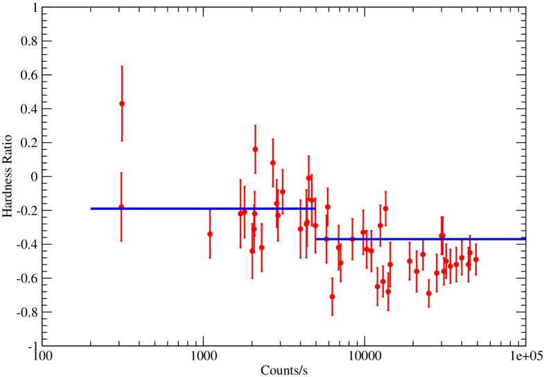
Figure 4: Hardness-intensity plot of the time resolved hardness ratio, Eq. (4.95). Data have been extract from Fig. 3 of Ref. [82]. Blue lines are our Eqs. (4.100) and (4.102).

Recently, it has been reported evidence for a hardness-intensity anti correlation within bursts from SGR 1806-20 [82]. Indeed, the authors of Ref. [82] reported observations of the soft gamma ray repeaters SGR 1806-20 obtained in October 2003, during a period of bursting activity. They found that some bursts showed a significant spectral evolution. However, in the present Section we focus on the remarkable correlation between hardness ratio and count rate. Following Ref. [82] we define the hardness ratio as:

$$HR\;=\frac{H\;-\;S}{H\;+\;S}\;\;\;,$$ (4.95)

where $H$ and $S$ are the background subtracted counts in the ranges $40-100\;KeV$ and $15-40\;KeV$ respectively. In Figure 4 we report the hardness ratio data extracted from Fig. 3 of Ref. [82]. A few comments are in order. First, the hardness ratio becomes negative for large enough burst intensities. Moreover, there is a clear decrease of the hardness ratio with increasing burst intensities. Note that, no detailed predictions are available within the standard magnetar model. On the other hand, within our approach we are able to explain why the hardness ratio is negative and decreases with increasing burst intensities. To see this, we note that the hardness ratio Eq. (4.95) is defined in terms of total luminosities in the relevant spectral intervals. Thus, to determine the total luminosity in the spectral interval $\omega_{1}-\omega_{2}$ we may use:

$$L(\omega_{1}-\omega_{2})\;=\;\int_{\omega_{1}}^{\omega_{2}}\;F(\omega)\;d\omega\;\;,$$ (4.96)

where $F(\omega)$ is given by Eq. (4.70). A straightforward integration gives:

$$L(\omega_{1}-\omega_{2})\;\simeq\;2\;\pi^{2}\;n_{e}\;e\;\frac{\delta B_{S}}{\delta t_{spike}}\;R^{4}\;\left(\frac{r_{1}}{R}\;-\;\frac{r_{2}}{R}\right)\;\;,$$ (4.97)

where $r_{1}$ and $r_{2}$ are given by:

$$\omega_{1,2}\;\simeq\;\gamma^{2}\;\frac{eB_{S}}{m_{e}}\;\left(\frac{R}{r_{1,2}}\right)^{3}\;\;\;.$$ (4.98)

Assuming $\gamma\thicksim 1$, we may rewrite Eq. (4.98) as:

$$\omega_{1,2}\;\simeq\;10\;MeV\;\left(\frac{R}{r_{1,2}}\right)^{3}\;\;\;.$$ (4.99)

Using Eqs. (4.97) and  (4.99) it is easy to determine the hardness ratio:

$$HR\;=\frac{L(40-100\;KeV)\;-\;L(15-40\;KeV)}{L(40-100\;KeV)\;+\;L(15-40\;KeV)}\;\simeq\;\frac{1.66\;-\;2.44}{1.66\;+\;2.44}\;\simeq\;-\;0.19\;\;.$$ (4.100)

In Figure 4 we display our estimate of the hardness ratio Eq. (4.100). We see that data are in quite good agreement with Eq. (4.100) at least up to count rate $\thicksim\,5\,10^{3}\;\frac{counts}{sec}$. For larger count rates data seem to lie below our value. We believe that, within our approach, there is a natural explanation for this effect. Indeed, for increasing count rates we expect that the hard tail $\omega\gtrsim 2\,m_{e}\simeq 1\,MeV$ of the spectrum will begin to contribute to the luminosity. According to the discussion in Sect. 4.3 these hard photons are reprocessed leading to an effective blackbody with temperature $T_{1}$. Now, for small and intermediate bursts the blackbody temperature $T_{1}$ is considerably smaller than Eq. (4.84), so that the effective blackbody contributes mainly to the soft tail of the spectrum. Obviously, the total luminosity of the effective blackbody is:

$$L(1-10\;MeV)\;\simeq\;2\;\pi^{2}\;n_{e}\;e\;\frac{\delta B_{S}}{\delta t_{spike}}\;R^{4}\;\left(2.15\;-\;1\right)\;\;.$$ (4.101)

Since this luminosity contributes to the soft part of the emission spectrum, Eq. (4.100) gets modified as:

$$HR\;\simeq\;\frac{1.66\;-\;3.59}{1.66\;+\;3.59}\;\simeq\;-\;0.37\;\;.$$ (4.102)

Equation (4.102) is displayed in Fig. 4 for rates $\gtrsim 5\,10^{3}\;\frac{counts}{sec}$. Note that we did not take into account the proton contribution to the luminosity. Observing that protons contribute mainly to luminosities at low energy $\omega\lesssim 10\,KeV$, we see that adding the proton contributions leads to smaller hardness ratios bringing our estimates to a better agreement with data. In any case, we see that our theory allows to explain in a natural way the puzzling anti correlation between hardness ratio and intensity.

5 LIGHT CURVES

In our magnetar theory the observed burst activities are triggered by glitches which inject magnetic energy into the magnetosphere where, as discussed in previous Sections, it is dissipated. As a consequence the observed luminosity is time depended. In this Section we set up an effective description which allows us to determine the light curves, i.e. the time dependence of the luminosity. In general, the energy injected into the magnetosphere after the glitch decreases due to dissipative effects described in Sect. 4.3, leading to the luminosity $L(t)=-\frac{dE(t)}{dt}$. Actually, the precise behavior of $L(t)$ is determined once the dissipation mechanisms are known. However, since the dissipation of the magnetic energy involves the whole magnetosphere, we may accurately reproduce the time variation of $L(t)$ without a precise knowledge of the microscopic dissipative mechanisms. Indeed, on general grounds we have that the dissipated energy is given by:

$$L(t)\;\;=\;\;-\;\frac{dE(t)}{dt}\;\;=\;\kappa(t)\;E^{\eta}\;\;,\;\;\eta\;\leq\;1\;\;\;,$$ (5.1)

where $\eta$ is the efficiency coefficient. Obviously the parameter $\kappa(t)$ does depend on the physical parameters of the magnetosphere. For an ideal system, where the initial injected energy is huge, the linear regime, where $\eta=1$, is appropiate. Moreover, we expect that the dissipation time $\thicksim\frac{1}{\kappa}$ is much smaller than the characteristic time needed to macroscopic modifications of the magnetosphere. Thus, we may safely assume $\kappa(t)\simeq\kappa_{0}$ constant. So that we get:

$$L(t)\;\;=\;\;-\;\frac{dE(t)}{dt}\;\;\simeq\;\kappa_{0}\;E\;\;.$$ (5.2)

It is straightforward to solve Eq. (5.2):

$$E(t)\;=\;E_{0}\;\exp(-\frac{t}{\tau_{0}})\;\;\;\;,\;\;\;L(t)\;=\;L_{0}\;\exp(-\frac{t}{\tau_{0}})\;\;,\;\;L_{0}\;=\;\frac{E_{0}}{\tau_{0}}\;\;,\;\;\tau_{0}\;=\;\frac{1}{\kappa_{0}}\;\;\;.$$ (5.3)

Note that the dissipation time $\tau_{0}=\frac{1}{\kappa_{0}}$ encodes all the physical information on the microscopic dissipative phenomena. Since the injected energy is finite, the dissipation of energy degrades with the decreasing of the available energy. Thus, the relevant equation is Eq. (5.1) with $\eta<1$. In this case, solving Eq. (5.1) we find:

$$L(t)\;=\;L_{0}\;\left(1-\frac{t}{t_{dis}}\right)^{\frac{\eta}{1-\eta}}\;\;,$$ (5.4)

where we have introduced the dissipation time:

$$t_{dis}\;\;=\;\;\frac{1}{\kappa_{0}}\;\frac{E_{0}^{1-\eta}}{1-\eta}\;\;.$$ (5.5)

Then, we see that the time evolution of the luminosity is linear up to some time $t_{break}$, after that we have a break from the linear regime $\eta=1$ to a non linear regime with $\eta<1$. If we indicate with $t_{dis}$ the total dissipation time, we get:

$$\begin{split}L(t)\;&=\;L_{0}\;\exp(-\frac{t}{\tau_{0}})\;\;\;\;\;\;,\;\;\;\;\;\;\;\;\;\;\;\;\;\;\;\;\;\;\;\;\;\;\;\;\;\;\;\;\;\;\;\;\;\;0\;<\;t\;<\;t_{break}\;\;,\\ L(t)\;&=\;L(t_{break})\;\left(1-\frac{t-t_{break}}{t_{dis}-t_{break}}\right)^{\frac{\eta}{1-\eta}}\;\;,\;\;\;\;\;\;\;\;\;t_{break}\;<\;t\;<\;t_{dis}\;\;.\end{split}$$ (5.6)

Equation (5.6) is relevant to describe the light curve after a giant burst, where there is a huge amount of magnetic energy dissipated into the magnetosphere. It is interesting to compare our light curves, Eq. (5.6), with the standard magnetar model. The decay of the luminosity in the standard magnetar model is due to the evaporation by a fireball formed after a giant burst and trapped onto the stellar surface [45, 83]. Indeed, the authors of Ref. [81] considered the light curves after the giant flare of 1998, August 27 from SGR 1900+14, and the giant flare of 1979 March 5 from SGR 0526-66. Assuming that the luminosity varies as a power of the remaining fireball energy $L\thicksim E^{a}$, they found:

$$L(t)\;=\;L_{0}\;\left(1-\frac{t}{t_{evap}}\right)^{\frac{a}{1-a}}\;\;,$$ (5.7)

where $t_{evap}$ is the time at which the fireball evaporates, and the index $a$ accounts for the geometry and the temperature distribution of the trapped fireball. For a spherical fireball of uniform temperature $a=\frac{2}{3}$, so that the index $a$ must satisfies the constrain:

$$a\;\leqslant\frac{2}{3}\;\;\;.$$ (5.8)

Note that our Eq. (5.6) reduces to Eq. (5.7) if $t_{break}=0$ and $\eta=a$. However, we stress that our efficiency exponent must satisfy the milder constraint $\eta\leqslant 1$.

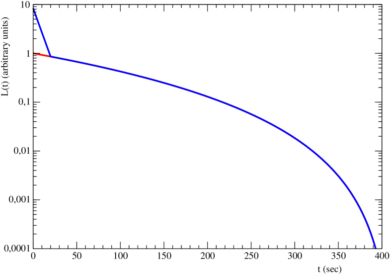
Figure 5: Light curve after the giant flare of 1998, August 27 from SGR 1900+14. Red continuous line is the light curve in the standard magnetar model, Eq. (5.7) with parameters given in Eq. (5.9). Blue line is our light curve Eq. (5.6) with parameters in Eq. (5.10)

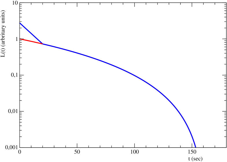
Figure 6: Light curve after the giant flare of 1979 March 5 from SGR 0526-66. Red continuous line is the light curve in the standard magnetar model, Eq. (5.7) with parameters given in Eq. (5.11). Blue line is our light curve Eq. (5.6) with parameters in Eq. (5.12)

The authors of Ref. [81] performed a best fit of the light curve of the August 27 flare, background subtracted and binned to $5\,sec$, to Eq. (5.7) and found:

$$a\;=\;0.756\;\pm\;0.003\;\;\;,\;\;\;t_{evap}\;=\;414\;sec\;\;\;.$$ (5.9)

Indeed, from Fig. 2 in Ref. [81] one sees that the trapped fireball light curve account for the decay trend of the experimental light curve and matches the sudden final drop of the flux. However, it should stressed that the fitting parameter $a$ in Eq. (5.9) does not satisfy the physical constraint Eq. (5.8). Even more, any deviations from spherical geometry or uniform temperature distribution lead to parameters $a$ smaller than the upper bound $\frac{2}{3}$. Moreover, the trapped fireball light curve underestimate by about an order of magnitude the measured flux during the first stage of the outburst. We interpreted the different behavior of the flux during the initial phase of the outburst as a clear indication of the linear regime described by our Eq. (5.3). As a matter of fact, we find that the measured light curve could be better described by Eq. (5.6) with parameters (see Fig. 5):

$$\tau_{0}\;=\;8.80\;sec\;\;,\;\;t_{break}\;=\;20\;sec\;\;,\;\;\;\eta\;=\;0.756\;\;\;,\;\;\;t_{dis}\;=\;414\;sec\;\;\;.$$ (5.10)

The same criticisms apply to the fit within the standard magnetar model of the light curve after the giant flare of 1979 March 5 from SGR 0526-66. The trapped fireball light curve fit in Ref. [81] gives:

$$a\;=\;0.71\;\pm\;0.01\;\;\;,\;\;\;t_{evap}\;=\;163\;\pm\;5\;sec\;\;\;.$$ (5.11)

Again the parameter $a$ exceeds the bound Eq. (5.8), and the fit underestimates the flux during the first stage of the outburst (see Fig. 14, Ref. [81]). Fitting our Eq. (5.6) to the measured flux reported in Fig. 14 of Ref. [81], we estimate:

$$\tau_{0}\;=\;15\;sec\;\;,\;\;t_{break}\;=\;20\;sec\;\;,\;\;\;\eta\;=\;0.71\;\;\;,\;\;\;t_{dis}\;=\;163\;sec\;\;\;.$$ (5.12)

In Figs. 5 and 6 we compare our light curves Eqs. (5.6), (5.10) and (5.12) with the best fits performed in Ref. [81]. Obviously, both light curves agree for $t>t_{break}$, while in the linear regime $t<t_{break}$, where the trapped fireball light curves underestimate the flux, our light curve follow the exponential decay and seem to be in closer agreement with observational data.

Several observations indicate that after a giant burst there are smaller and recurrent bursts. According to our theory these small and recurrent bursts are the effect of several small glitches following the giant glitch. We may think about these small bursts like the seismic activity following a giant earthquake. These seismic glitches are characterized by light curves very different from the giant burst light curves. In the standard magnetar model these light curves are accounted for with an approximate $t^{-0.7}$ decay [84]. Below we compare this prediction with observations and argue that the standard theory is unable to adequately describe observational data. On the other hand, within our theory there is a natural way to describe the seismic burst activity. Indeed, during these seismic bursts, that we shall call settling bursts, there is an almost continuous injection of energy into the magnetosphere which tends to sustain an almost constant luminosity. This corresponds to an effective $\kappa$ in Eq. (5.1) which decreases smoothly with time. The simplest choice is:

$$\kappa(t)\;=\;\frac{\kappa_{0}}{1+\kappa_{1}t}\;\;\;.$$ (5.13)

Inserting into Eq. (5.1) and integrating, we get:

$$E(t)\;=\;\left[E_{0}^{1-\eta}\;-(1-\eta)\;\frac{\kappa_{0}}{\kappa_{1}}\;\ln(1+\kappa_{1}t)\right]^{\frac{\eta}{1-\eta}}\;\;\;.$$ (5.14)

So that the luminosity is:

$$L(t)\;=\;\frac{L_{0}}{(1+\kappa_{1}t)^{\eta}}\;\left[1\;-(1-\eta)\;\frac{\kappa_{0}}{\kappa_{1}E_{0}^{1-\eta}}\;\ln(1+\kappa_{1}t)\right]^{\frac{\eta}{1-\eta}}\;\;\;.$$ (5.15)

After defining the dissipation time:

$$\ln(1+\kappa_{1}t_{dis})\;=\;\frac{\kappa_{1}}{\kappa_{0}}\;\frac{E_{0}^{1-\eta}}{1-\eta}\;\;\;,$$ (5.16)

we rewrite Eq. (5.15) as

$$L(t)\;=\;\frac{L_{0}}{(1+\kappa_{1}t)^{\eta}}\;\left[1\;-\;\frac{\ln(1+\kappa_{1}t)}{\ln(1+\kappa_{1}t_{dis})}\right]^{\frac{\eta}{1-\eta}}\;\;\;.$$ (5.17)

Note that the light curve Eq. (5.17) depends on two characteristic time constants $\frac{1}{\kappa_{1}}$ and $t_{dis}$. We see that $\kappa_{1}t_{dis}$, which is roughly the number of small bursts occurred in the given event, gives an estimation of the seismic burst intensity. Moreover, since during the seismic bursts the injected energy is much smaller than in giant bursts, we expect that fitting Eq. (5.17) to the observed light curves will result in values of $\eta$ smaller than the typical values in giant bursts. In the following Sections we show that, indeed, our light curves Eq. (5.17) are in good agreement with several observations.

5.1 AXP 1E 2259+586

On 2002, June 18 SGR-like bursts was recorded from AXP 1E 2259+586. Coincident with the burst activity were gross changes in the pulsed flux, persistent flux, energy spectrum, pulse profile and spin down of the source [60]. As discussed in previous Sections, these features are naturally accounted for within our theory. However, we believe that the most remarkable and compelling evidence for our proposal comes from the observed coincidence of the burst activity with a large glitch. Moreover, the time evolution of the unabsorbed flux from AXP 1E 2259+586 following the 2002 June outburst reported in Ref. [60] can be explained naturally within our theory, but it is completely unreachable within the standard magnetar theory. So that we consider the June 18 SGR-like bursts from AXP 1E 2259+586 the Rosetta Stone for our magnetar theory.
The temporal decay of the flux during the burst activity displays a rapid initial decay which lasted about $1\;days$, followed by a more mild decay during the year following the onset of the burst activity. Indeed, the authors of Ref. [60] splitted the data into two segments, and fit each independently to a power law:

$$\begin{split}F(t)\;&\;\;\thicksim\;\;t^{\alpha_{1}}\;\;,\;\alpha_{1}\;=\;-\;4.8\;\pm\;0.5\;\;\;\;\;\;,\;\;t\;\lesssim 1\;\;days\;\;\;,\\ F(t)\;&\;\;\thicksim\;\;t^{\alpha_{2}}\;\;,\;\alpha_{2}\;=\;-\;0.22\;\pm\;0.01\;\;\,,\;\;t\;\gtrsim 1\;\;days\;\;\;.\end{split}$$ (5.18)

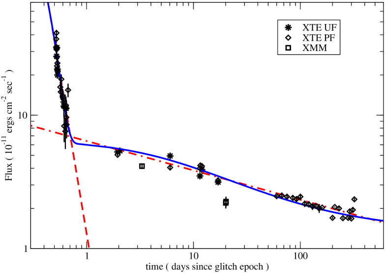
Figure 7: The time evolution of the unabsorbed flux from AXP 1E 2259+586 following the 2002 June outburst. Data have been extracted from Fig. 13 in Ref. [60]. Red dashed and dot-dashed lines are the phenomelogical power law fits, Eq. (5.18). Blue continuous line is our light curve Eq. (5.20), with parameters in Eq. (5.23).

It is evident from Eq. (5.18) that the standard magnetar model is completely unable to reproduce the phenomelogical power law fit. On the other hand, even the phenomenological parametrization cannot account for the time evolution of the flux. Indeed, if we assume the power law Eq. (5.18) for the decay of the flux, then we cannot explain why and how the source returns in its quiescent state with quiescent flux [60]:

$$F_{Q}\;\;\simeq\;\;1.53\;10^{-11}\;\frac{ergs}{cm^{2}\,sec}\;\;.$$ (5.19)

Note that adding the quiescent flux to the power law decay does not resolve the problem, for in that case the fits worst considerably. Our interpretation of the puzzling light curve displayed in Fig.7 is that AXP 1E 2259+586 has undergone a giant burst at the glitch epoch, and soon after the pulsar has entered into a intense seismic burst activity. Accordingly, the flux can be written as:

$$F(t)\;=\;F_{GB}(t)\;+\;F_{SB}(t)\;+\;F_{Q}\;\;\;\;,$$ (5.20)

where $F_{Q}$ is the quiescent flux, Eq. (5.19), $F_{GB}(t)$ is the giant burst contribution to the flux given by Eq. (5.6), and $F_{SB}(t)$ is the seismic burst contribution given by Eq. (5.17). Since during the first stage of the outburst there are no available data, we may parameterize the giant burst contribution as:

$$F_{GB}(t)\;=\;F_{GB}(0)\;\left(1-\frac{t}{t_{GB}}\right)^{\frac{\eta_{GB}}{1-\eta_{GB}}}\;\;,\;\;\;0\;<\;t\;<\;t_{GB}\;\;,$$ (5.21)

while $F_{SB}(t)$ is given by:

$$F_{SB}(t)\;=\;\frac{F_{SB}(0)}{(1+\kappa_{1}t)^{\eta_{SB}}}\;\left[1\;-\;\frac{\ln(1+\kappa_{1}t)}{\ln(1+\kappa_{1}t_{SB})}\right]^{\frac{\eta_{SB}}{1-\eta_{SB}}}\;\;,\;\;\;0\;<\;t\;<\;t_{SB}\;\;\;,$$ (5.22)

where $t_{GB}$ and $t_{SB}$ are the dissipation time for giant and seismic bursts respectively. In Fig. 7 we display our light curve Eq. (5.20) with the following parameters:

$$\begin{split}F_{GB}(0)\;&\simeq\;1.5\;10^{-8}\;\frac{ergs}{cm^{2}\,sec}\;\;,\;\;\eta_{GB}\;\simeq\;0.828\;\;,\;\;t_{GB}\;\simeq\;0.91\;days\;\\ F_{SB}(0)\;&\simeq\;5.0\;10^{-11}\;\frac{ergs}{cm^{2}\,sec}\;,\;\eta_{SB}\;\simeq\;0.45\;,\;t_{SB}\;\simeq\;10^{3}\;days\;,\;\kappa_{1}\;\simeq\;0.20\;days^{-1}\;.\end{split}$$ (5.23)

A few comments are in order. First, the agreement with data is rather good. Second, our efficiency exponent $\eta_{GB}$ is consistent with the values found in the giant bursts from SGR 1900+14 and SGR 0526-66, and cannot be justify in the standard magnetar model. On the other hand, quite consistently, we have $\eta_{SB}<\eta_{GB}$. Finally, we stress that from our interpretation of the light curve it follows that the onset of the intense seismic burst activity ($\kappa_{1}t_{SB}\sim 200$) did not allow a reliable estimation of $\frac{\delta\dot{\nu}}{\dot{\nu}}$, which we predicted to be of order $10^{-2}$.

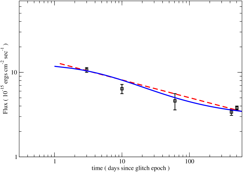
Figure 8: The time evolution of the unabsorbed IR flux from AXP 1E 2259+586 following the 2002 June outburst. Data have been extracted from Fig. 1 in Ref. [85]. Red dashed line is the phenomelogical power law fit $t^{-0.21\pm 0.01}$. Blue continuous line is our light curve Eq. (5.24).

Interestingly enough, following the 2002 June outburst it was detected a infrared flux changes correlated with the $X$-ray flux variability [85]. Since the observations began three days after the 2002 June outburst, according to our theory the infrared flux is parameterized as:

$$F_{SB}^{IR}(t)\;=\;\frac{F_{SB}^{IR}(0)}{(1+\kappa_{1}t)^{\eta_{SB}}}\;\left[1\;-\;\frac{\ln(1+\kappa_{1}t)}{\ln(1+\kappa_{1}t_{SB})}\right]^{\frac{\eta_{SB}}{1-\eta_{SB}}}\;\;+\;\;F_{Q}^{IR}\;\;,\;\;\;0\;<\;t\;<\;t_{SB}\;\;,$$ (5.24)

with the same parameters as in Eq. (5.22). Indeed, assuming $F_{SB}^{IR}(0)\simeq 9.5\;10^{-15}\frac{ergs}{cm^{-2}sec^{-1}}$ and $F_{Q}^{IR}\simeq 3.3\;10^{-15}\frac{ergs}{cm^{-2}sec^{-1}}$, we found that our light curve Eq. (5.24) is in remarkable good agreement with data (see Fig. 8). The strong correlation between infrared and $X$-ray flux decay observed after the 2002 June outburst from AXP 1E 2259+586 strongly suggest a physical link between the origin of both type of radiation. In particular, this unambiguously implies that the infrared flux originates from the magnetosphere. Indeed, in Appendix we argue that the soft emission from gamma-ray repeaters, anomalous $X$-ray pulsars, and isolated $X$-ray pulsars originates from thermal photons reprocessed by electrons trapped above the polar cups. On the other hand, we have already shown that the burst activity produces an increases of the thermal flux from the pulsar surface. So that, we see that in our theory the observed correlation between infrared and $X$-ray flux decays finds a natural explanation.

5.2 SGR 1900+14

Soon after the 1998, August 27 giant burst, the soft gamma repeater SGR 1900+14 entered a remarkable phase of activity. On August 29 an unusual burst from SGR 1900+14 was detected [86] which lasted for a long time $\thicksim 10^{3}sec$. As discussed in Ref. [86], on observational grounds it can be ruled out extended afterglow tails following ordinary bursts. Moreover, the standard magnetar model predicts faint transient afterglows on a time scale comparable to the duration of the bright $X$-ray emission of the burst peak. So that such mechanism cannot explain the long extended afterglow tail of August 29.

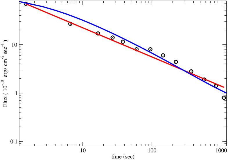
Figure 9: Flux evolution of the August 29 burst from SGR 1900+14. Data has been extracted from Fig. 4, panel (d), of Ref. [86]. Red line is the phenomenological power law fit Eq. (5.25); blue line is our light curve Eqs. (5.27) and (5.28).

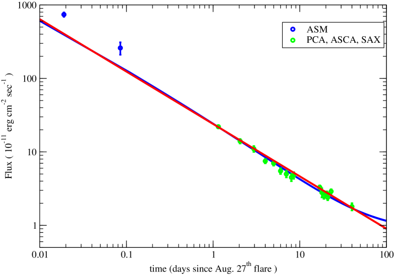
Figure 10: The time evolution of the unabsorbed flux from SGR 1900+14 following the 1998 August outburst. Data has been extracted from Fig. 2 of Ref. [88]. Red line is the power law best fit $F(t)\thicksim t^{-(0.713\pm 0.025)}$. Blu line is our light curve Eqs. (5.27) and (5.29).

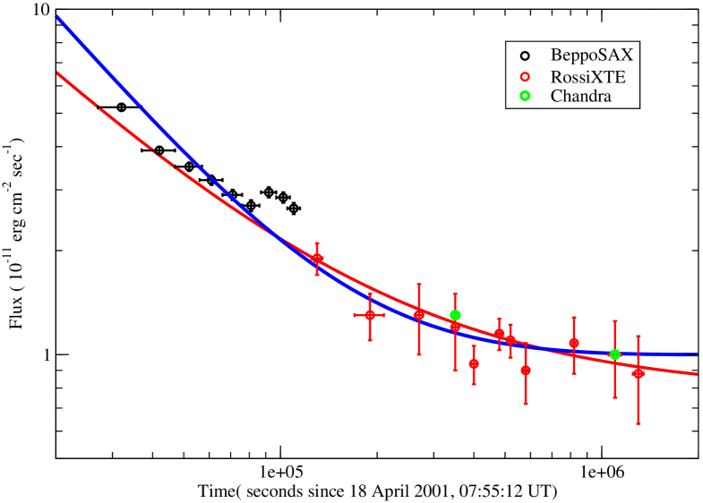
Figure 11: Temporal behavior of the $X$-ray flux from SGR 1900+14 in the aftermath of the 2001 April 18 flare. Data have been extracted from Fig. 2 of Ref. [89]. Red line is the power law best fit Eqs. (5.30) and (5.31). Blu line is our light curve Eqs. (5.27) and (5.32).

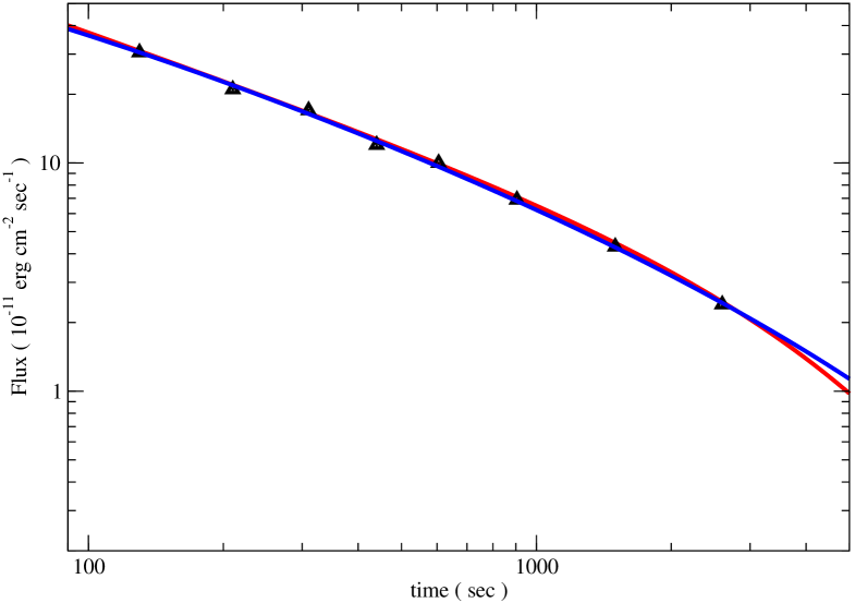
Figure 12: The temporal decay of the flux from the 2001 April 28 burst from SGR 1900+14 in the energy band $2-20\;KeV$. The data has been extracted from Fig. 5 of Ref. [90]. Red continuous line is the phenomenological best-fit power law times exponential function adopted in Ref. [90] to describe data, Eqs. (5.33) and (5.34). Blue continuous line is our light curve Eqs. (5.27) and (5.35).

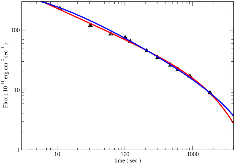
Figure 13: The temporal decay of the flux from the 1998 August 29 burst from SGR 1900+14 in the energy band $2-20\;KeV$. The data has been extracted from Fig. 10 of Ref. [90]. Red continuous line is the phenomenological best-fit power law times exponential function adopted in Ref. [90] to describe data, Eqs. (5.33) and (5.36). Blue continuous line is our light curve Eqs. (5.27) and (5.37).

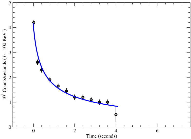
Figure 14: Time history of the 2001 July 2 burst from SGR 1900+14 in the energy band $7-100\;KeV$ as observed by FREGATE. The data has been extracted from Fig. 1 of Ref. [91] by binning the light curve histogram. Blue continuous curve is our light curve Eqs. (5.27) and (5.38).

In Figure 9 we display the flux decay after the August 29 burst. Data has been extracted from Ref. [86]. In Ref. [86] the temporal behavior of the flux decay has been parameterized as a power law (red line in Fig. 9):

$$F(t)\;\;=\;\;(89.16\;\pm\;1.34)\;10^{-10}\;\frac{ergs}{cm^{2}\,sec}\;t^{-(0.602\pm 0.025)}\;.$$ (5.25)

As already stressed, the phenomenological power law decay cannot explain the return of the source in its quiescent state where the flux is [87]:

$$F_{Q}\;\;=\;\;0.96\;\pm 0.07\;10^{-11}\;\frac{ergs}{cm^{2}\,sec}\;\;.$$ (5.26)

On the other hand, we may easily account for the observed flux decay by our light curve:

$$F(t)\;=\;\frac{F(0)}{(1+\kappa_{1}t)^{\eta}}\;\left[1\;-\;\frac{\ln(1+\kappa_{1}t)}{\ln(1+\kappa_{1}t_{dis})}\right]^{\frac{\eta}{1-\eta}}\;\;+\;\;F_{Q}\;\;,$$ (5.27)

where $F_{Q}$ is fixed by Eq. (5.26). Indeed, in Fig. 9 we compare our light curve Eq. (5.27) with observational data. The agreement is quite satisfying if we take:

$$F(0)\;\simeq\;1.05\;10^{-9}\;\frac{ergs}{cm^{2}\,sec}\;,\;\eta\;\simeq\;0.5\;,\;t_{dis}\;\simeq\;1.2\;10^{3}\;sec\;,\;\kappa_{1}\;\simeq\;0.50\;sec^{-1}\;.$$ (5.28)

The authors of Ref. [88] have analyzed a large set of $X$-ray observations of SGR 1900+14 in order to construct a more complete flux history. They found that the flux level was more than an order of magnitude brighter than the level during quiescence. This transient flux enhancement lasts about $40\;days$ after the giant flare. Unlike the authors of Ref. [88], which argued that this enhancement was an artifact of the August 27 flare, we believe that the flux history can be adequately described as seismic burst activity of the source. In Fig. 10 we report the flux light curve extracted from Fig.2 of Ref. [88] together with their power law best fit. Again we find the the flux history is accounted for quite well by our light curve Eq. (5.27) with the following parameters:

$$F(0)\;\simeq\;4.8\;10^{-8}\;\frac{ergs}{cm^{2}\,sec}\;,\;\eta\;\simeq\;0.55\;,\;t_{dis}\;\simeq\;200\;days\;,\;\kappa_{1}\;\simeq\;2\;10^{3}\;days^{-1}\;.$$ (5.29)

The agreement between our light curve Eqs. (5.27) and (5.29) with the power law best fit is striking. Moreover we see that our curve deviates from the power law fit for $t>60\;days$ tending to $F_{Q}$ at $t=t_{dis}$. The authors of Ref. [88] noted that extrapolating the fit to the August 27 $X$-ray light curve back toward the flare itself, one finds that the expected flux level lies below the ASM flux measurements (blue open points in Fig. 10). Moreover, these authors observed that the discrepancy reduces somewhat when one pushes forward the reference epoch to about 14 minutes after the onset of the flare. However, unlike the authors of Ref. [88] we believe that the discrepancy is due to a true physical effect, namely the observed discrepancy from extrapolated light curve and ASM measurements is a clear indication that the surface luminosity increases after the burst activity. In particular, soon after the August 27 giant flare we have seen in Sect. 4.3 that the surface temperature increases up to $\thicksim 61\;KeV$ and the surface luminosity reaches $\thicksim 10^{44}\;\frac{erg}{sec}$. Almost all the deposited energy is dissipated within the dissipation time of the giant flare $\thicksim 400\;sec$. Nevertheless, it is natural to expect a more gradual afterglow where a small fraction of the energy deposited onto the star surface is gradually dissipated. As a matter of fact, we find that the observed level of luminosity $L_{X}\,\thicksim\,10^{38}\;\frac{erg}{sec}$ (assuming a distance $d=10\;kpc$) at about $0.01\;days$ since the August 27 giant flare, is consistent with the gradual afterglow scenario.

On 2001 April 18 the soft gamma ray repeater SGR 1900+14 emitted an intermediate burst. The light curve of this event did not show any initial hard spike and was clearly spin-modulated. Moreover, the energetics appeared to be intermediate in the $40-700\,KeV$ range, with a total emitted energy of about $1.9\;10^{42}\;ergs$ [89]. In Fig. 11 we report the temporal behavior of the $X$-ray ($2-10\;KeV$) flux from SGR 1900+14 in the aftermath of the 2001 April 18 flare. Data has been extracted from Fig. 2 of Ref. [89]. The authors of Ref. [89] attempted a simple power law function to the flux data:

$$F(t)\;\thicksim\;t^{-\alpha}\;\;+\;\;K\;\;,$$ (5.30)

where the constant $K$ should take care of the quiescent luminosity. Indeed, the authors of Ref. [89] fitting Eq. (5.30) to the data found:

$$\alpha\;=0.89(6)\;\;\;,\;\;K\;=\;0.78(5)\;10^{-11}\;\;\frac{ergs}{cm^{2}\,sec}\;\;.$$ (5.31)

As it is evident from Fig. 11, the power law globally fits the data quite nicely. However, the reduced $\chi^{2}$ turns out to be in excess to $3$, mainly due to the bump occurring in the light curve at $t\thicksim 10^{5}\,sec$ [89]. Indeed, after excluding the bump they get a good fit with $\chi^{2}/dof\simeq 1$ without an appreciable variation of the fit parameters [89]. However, there is still a problem with the phenomelogical power law decay of the flux. As a matter of fact, Eq. (5.31) shows that the power law fit underestimates the quiescent luminosity. In our opinion this confirms that the phenomenological power law decay of the flux is not adeguate to describe the time variation of the flux. On the other hand, we find that our light curve Eq. (5.27), with quiescent luminosity fixed to the observed value Eq. (5.26), furnishes a rather good description of the flux decay once the parameters are given by:

$$F(0)\;\simeq\;2.6\;10^{-7}\;\frac{ergs}{cm^{2}\,sec}\;,\;\eta\;\simeq\;0.68\;,\;t_{dis}\;\simeq\;3\;10^{6}\;sec\;,\;\kappa_{1}\;\simeq\;0.25\;sec^{-1}\;.$$ (5.32)

Within our interpretation, Eq. (5.32) shows that the flux decay in the aftermath of the April 18 flare is characterized by a very large seismic burst activity ($\kappa_{1}t_{dis}\thicksim 10^{6}$), which lasts for about $10^{6}\;sec$. So that the bump in the flux at $t\thicksim 10^{5}\,sec$ is naturally explained as fluctuations in the intensity of the seismic bursts.

In Ref. [90] it is reported the spectral evolution and temporal decay of the $X$-ray tail of a burst from SGR 1900+14 recorded on 2001 April 28, 10 days after the intense April 18 event. In Fig. 12 we display the temporal decay of the flux from the 2001 April 28 burst in the energy band $2-20\;KeV$. The data has been extracted from Fig. 5 of Ref. [90]. These authors attempted several functional forms to fit the decay of the flux. They reported that the decay was equally well fitted by a either power law times exponential or broken power law. We stress that both fits are phenomenological parametrization of the observational data, and that both fits are unable to recover the quiescent flux. For definitiveness, we shall compare our light curve with the power law times exponential fit:

$$F(t)\;\thicksim\;t^{-\alpha}\;\exp(-\frac{t}{\tau})\;\;\;\;,$$ (5.33)

The best fit to the temporal decay of the flux from the 2001 April 28 burst in the energy band $2-20\;KeV$ gives [90]:

$$\alpha\;=0.68\;\pm\;0.04\;\;\;\;,\;\;\;\;\tau\;=\;5\;\pm\;1\;10^{3}\;sec\;\;\;\;.$$ (5.34)

In Figure 12 we compare the phenomenological best fit Eqs. (5.33) and (5.34) with our light curve Eq. (5.27), where the quiescent luminosity is fixed to the observed value Eq. (5.26), and the parameters are given by:

$$F(0)\;\simeq\;1.4\;10^{-9}\;\frac{ergs}{cm^{2}\,sec}\;,\;\eta\;\simeq\;0.5\;,\;t_{dis}\;\simeq\;5.5\;10^{3}\;sec\;,\;\kappa_{1}\;\simeq\;0.06\;sec^{-1}\;.$$ (5.35)

Again, we see that our light curve gives a quite satisfying description of the flux decay.

Interestingly, the authors of Ref.[90] analyzed with the same techniques the 1998 August 29 burst from SGR 1900+14. The fit to the decay of the flux in the energy band $2-20\;KeV$ with Eq. (5.33) resulted in:

$$\alpha\;=\;0.510\;\pm\;0.008\;\;\;,\;\;\;\tau\;=\;2.9\;\pm\;0.2\;10^{3}\;sec\;\;\;\;.$$ (5.36)

Even in this case our light curve is able to follow the time decay of the flux in a satisfying way. In Fig. 13 we compare our light curve with parameters:

$$F(0)\;\simeq\;5.0\;10^{-9}\;\frac{ergs}{cm^{2}\,sec}\;,\;\eta\;\simeq\;0.45\;,\;t_{dis}\;\simeq\;7.0\;10^{3}\;sec\;,\;\kappa_{1}\;\simeq\;0.25\;sec^{-1}\;,$$ (5.37)

and the phenomelogical power law times exponential fit Eqs. (5.33) and (5.36).

Let us consider, finally, the light curve for the intermediate burst from SGR 1900+14 occurred on 2001 July 2 [91]. In Figure 14 we display the time decay of the flux after the July 2 burst. The data have been extracted from Fig. 1 of Ref. [91] by binning the light curve histogram. The displayed errors are our estimate, so that the data should be considered as purely indicative of the decay of the flux. We find that Fig. 1 of Ref.[91] is very suggestive, for it seem to indicate that the burst results from several small bursts, i.e. according to our theory the burst is a seismic burst. As a consequence we try the fit with our light curve Eq. (5.27). In this case the quiescent flux has been fixed to $F_{Q}\simeq 0$, for the observational data has been taken in the energy range $7-100\;KeV$ where the quiescent flux is very small. Attempting the fit to the data we find:

$$F(0)\;\simeq\;4.07\;10^{4}\;\frac{counts}{sec}\;,\;\eta\;\simeq\;0.36\;,\;t_{dis}\;\simeq\;40\;sec\;,\;\kappa_{1}\;\simeq\;5.0\;sec^{-1}\;.$$ (5.38)

The resulting light curve is displayed in Fig. 14. The peculiarity of this burst resides in the fact that the burst activity terminates suddenly at $t\simeq 4\;sec$ well before the natural end at $t_{dis}\simeq 40\;sec$.

5.3 SGR 1627-41

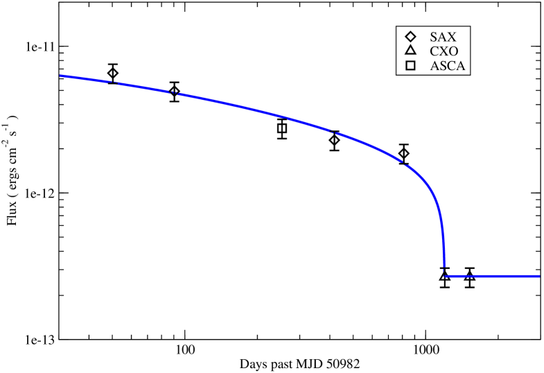
Figure 15: Time decay of the flux from SGR 1627-41. The data has been taken from Table 1 of Ref. [94]. Blue continuous line is our best fitted light curve Eqs. (5.27), (5.39) and (5.40).

SGR 1627-41 was discovered with the Burst And Transient Source Experiment (BATSE) on the Compton Gamma-Ray Observatory (CGRO) in June 1998 [92, 93] when it emitted over 100 bursts within an interval of 6 weeks. The authors of Ref [94] presented the results of the monitoring of the flux decay of the $X$-ray counterpart of SGR 1627-41 spanning an interval of roughly five years. Moreover, these authors attempted to understand the three year monotonic decline of SGR 1627-41 as cooling after a single deep crustal heating event coinciding with the burst activity in 1998 within the standard magnetar model. They assumed an initial energy injection to the crust of the order of $10^{44}\;ergs$. However, it must be pointed out that this assumption is highly unrealistic, for the estimate of the total energy released in bursts during the activation of SGR 1627-41 range between $4\;10^{42}-2\;10^{43}\;ergs$. In addition, since gamma rays was not detected, they assume that the conversion efficiency of the total energy released during the activation into soft gamma rays were considerable less than $100\;\%$. They also assumed that the core temperature is low, i.e. the core cools via the direct URCA process [30]. Notwithstanding these rather ad hoc assumptions, the authors of Ref. [94] was unable to explain the March 2003 data point, which clearly showed that the flux did not decay further (see Fig. 15). In other words, the levelling of the flux during the third year followed by its sharp decline is a feature that is challenging that standard magnetar model based on neutron stars, and that beg for an explanation within that model. On the other hand, we now show that the peculiar SGR 1627-41 light curve find a natural interpretation within our theory. In Fig. 15 we display the time decay of the flux. The data has been taken from Table 1 of Ref. [94]. In this case we are able to best fit our light curve Eq. (5.27) to available data. Since the number of observations is rather low, to get a sensible fit we have fixed the dissipation time to $1200\;days$ and the quiescent luminosity to the levelling value at $t\gtrsim 1200\;days$:

$$F_{Q}\;\simeq\;2.7\;10^{-13}\;\frac{ergs}{cm^{2}\,sec}\;\;\;,\;\;\;t_{dis}\;\simeq\;1200\;days\;\;.$$ (5.39)

The best fit of our light curve to data gives:

$$F(0)\;=\;0.83(11)\;10^{-11}\;\frac{ergs}{cm^{2}\,sec}\;,\;\eta\;=\;0.25(8)\;,\;\kappa_{1}\;=\;0.04(1)\;days^{-1}\;.$$ (5.40)

with a reduced $\chi^{2}\,\thicksim\,1$. From Fig. 15, where we compare our best fitted light curve with data, we see that our theory allow a quite satisfying description of the three year monotonic decline of the flux.

5.4 SGR 1806-20

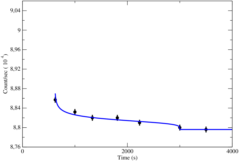
Figure 16: Time history of the second component after the 2004 December 27 giant burst from SGR 1806-20. The data has been extracted from Fig. 5 of Ref. [95] by binning the light curve histogram. Blue continuous curve is our light curve Eqs. (5.27), (5.42) and (5.43).

SGR 1806-20 entered an active phase in 2003, culminating in a gigantic flare on 2004 December 27, with energy greatly exceeding that of all previous events. In Figure 3 of Ref. [80] it is reported the time history of the flux averaged over the rotation period of the pulsar soon after the giant flare. These authors fitted the light curve within the standard magnetar model based on the evaporation of a fireball formed after the giant burst and trapped onto the stellar surface, Eq. (5.7). The fit of the rotation smoothed curve to the fireball function gives [80]:

$$a\;=\;0.606\;\pm\;0.003\;\;\;,\;\;\;t_{evap}\;=\;382\;\pm\;3\;\;sec\;\;\;.$$ (5.41)

However, from Figure 3 of Ref. [80] it is evident that fireball light curve underestimate the luminosity for $t\lesssim 30\;sec$. Thus we see that the light curve can be better accounted for by our light curve Eq. (5.6) with $t_{break}\simeq 30\;sec$, quite close to the values found for the giant bursts from SGR 1900+14 and SGR 0526-66. A more precise determination of the parameters of our light curve, however, must await for more precise data in the initial phase of the afterglow. Instead, in the present Section we discuss the light curve of a second, separate component after the giant burst reported in Ref. [95]. The authors of Ref. [95] found evidence for a separate component in the light curve starting at $t\thicksim 400\;sec$ from the onset of the giant burst, forming a peak at $t\thicksim 600\;sec$ and ending at $t\thicksim 3000\;sec$ (see Fig. 5 of Ref. [95]). As already discussed, in our theory it is expected that there is a intense seismic burst activity following a giant burst. In Figure 16 we display the flux history starting from the giant flare. We show a few point of the second component extracted from Fig. 5 of Ref. [95] by binning the light curve histogram. The displayed errors are our estimate, so that the data should be considered as purely indicative of the decay of the flux. We fit the data with our light curve Eqs. (5.27) assuming:

$$F_{Q}\;\simeq\;8.796\;10^{4}\;\frac{count}{sec}\;\;,\;\;t_{dis}\;=\;t_{end}\;-\;t_{start}\;\;,\;\;t_{start}\;\simeq\;625\;sec\;\;,\;\;t_{end}\;\simeq\;3000\;sec\;\;.$$ (5.42)

The best fit of our light curve to data gives:

$$F(0)\;=\;0.074\;10^{4}\;\frac{count}{sec}\;,\;\eta\;=\;0.18\;,\;\kappa_{1}\;=\;0.10\;sec^{-1}\;.$$ (5.43)

Indeed, in Fig. 16 we compare our light curve with data and find that our theory allow a quite satisfying description of the time history of the flux.

6 CONCLUSIONS

Let us summarize the main results of the present paper. We have discussed p-stars endowed with super strong dipolar magnetic field. We found a well defined criterion to distinguish rotation powered pulsars from magnetic powered pulsars (magnetars). We showed that glitches, that in our magnetars are triggered by magnetic dissipative effects in the inner core, explain both the quiescent emission and bursts from soft gamma-ray repeaters and anomalous $X$-ray pulsars. In particular, we were able to account for the braking glitch from SGR 1900+14 and the normal glitch from AXP 1E 2259+586 following a giant burst. We accounted for the observed puzzling anti correlation between hardness ratio and intensity. Within our magnetar theory we were able to account quantitatively for light curves for both gamma-ray repeaters and anomalous $X$-ray pulsars. In particular we explained the light curve after the June 18, 2002 giant burst from AXP 1E 2259+586. Finally, in Appendix we discussed the origin of the soft emission from soft gamma-ray repeaters, anomalous $X$-ray pulsars, isolated $X$-ray pulsars.
We believe that anomalous $X$-ray pulsars and soft gamma-ray repeaters are two class of intriguing objects that are challenging the standard paradigm based on neutron stars. In the present paper we convincingly argued that the standard magnetar theory is completely unable to account for the observational properties of anomalous $X$-ray pulsars and soft gamma-ray repeaters. On the other hand, we feel that the ability of our p-star theory to reach a complete understanding of several observational features of soft gamma-ray repeaters and anomalous $X$-ray pulsars strongly supports our proposal for a drastic revision of the standard paradigm of relativistic astrophysics.
Let us conclude by briefly addressing the theoretical foundation of our theory. As a matter of fact, our proposal for p-stars stems from recent numerical lattice results in QCD [96, 97], which suggested that the gauge system gets deconfined in strong enough chromomagnetic field. This leads us to consider the new class of compact quark stars made of almost massless deconfined up and down quarks immersed in a chromomagnetic field in $\beta$-equilibrium. Our previous studies showed that these compact stars are more stable than neutron stars whatever the value of the chromomagnetic condensate. This remarkable result indicates that the true ground state of QCD in strong enough gravitational field is not realized by hadronic matter, but by p-matter. In other words, the final collapse of an evolved massive star leads inevitably to the formation of a p-star.

Appendix A ORIGIN OF THE SOFT EMISSION IN $X$-RAY PULSARS

A number of anomalous $X$-ray pulsars have recently been detected in the optical-infrared wavelengths (for a recent review, see Ref. [98]). Since pulsar surface emission cannot account for the observed soft emission spectra, the emission must be magnetospheric in origin. This is clearly demonstrated by the correlation of the infrared flux with the bursting activity recently observed for the anomalous $X$-ray pulsar AXP 1E 2259+586 [85] (see Sect. 5.1). Remarkably, there is compelling evidence for an excess of the flux in the infrared band in anomalous $X$-ray pulsars with respect to the thermal component extrapolated from $X$-ray data. Up to now the standard magnetar model, is unable to account for the observed infrared emission or variability. In any case, irrespective to the actual mechanism responsible for the soft emission there is no doubt that the optical-infrared emission originates in the magnetosphere. Looking at the broad band energy spectrum of anomalous $X$-ray pulsars one realizes quickly that the spectra are amazingly similar to the ones of isolated $X$-ray pulsars, like RXJ 1856.5-3754 or RXJ 0720.4-3125. This strongly suggest that it must exist some natural mechanism capable to generate the soft tail of the spectrum of isolated pulsar, anomalous $X$-ray pulsars and soft gamma ray repeaters. In Refs. [9, 10] we already advanced the proposal that the faint emissions from RXJ 1856.5-3754 and RXJ 0720.4-3125 originate in the magnetosphere from synchrotron radiation emitted by electrons. That proposal was based on the observational fact that the faint emission can be parameterized quite well by a non thermal power law. However, we did not address the problem of the physical mechanism which is at the heart of the electron energy spectrum needed to generate the power law emission. In this Appendix we shall discuss a fair natural mechanism which is able to explain the faint emission for isolated pulsars as well as anomalous $X$-ray pulsars and soft gamma ray repeaters. In our mechanism the power law emission in the infrared-optical band is due to thermal radiation reprocessed in the magnetosphere by electrons trapped near the magnetic polar cups.
To start with, let us consider the motion of a charged particle in the pulsar magnetic dipolar field. We are assuming the presence of neutral plasma formed by electrons and protons with number densities $n_{e}=n_{p}$. Now, as is well known, for strong enough magnetic fields the plasma near the stellar surface will be channelled toward the magnetic pole. So that we are led to consider the motion of charged particles which are drifting toward the magnetic polar cups. Further, we may consider a polar region with area small enough such that the dipolar magnetic field depends only on the distance from the surface. If the magnetic polar axis is in direction $z$, then charged particles moving towards the stellar surface will feel an almost uniform magnetic field having z-component $B(z)$. Thus we are led to consider the motion of charge particle in the magnetic field:

$$B(z)\;=\;-\;B_{S}\;\frac{R^{3}}{z^{3}}\;\;,\;z\;\geq\;R\;\;,$$ (A.1)

where, for the sake of definitiveness we are considering the north magnetic pole where the magnetic field is entering into the stellar surface. Let us consider, firstly, electron with charge $-e$ and mass $m_{e}$. The electron wave function $\psi(x,y,z)$ can be obtained by solving the Schrödinger equation in presence of the magnetic field $B(z)$. We are interested in the physical problem where an electron, starting from a distance $z_{0}$ from the star, is approaching the stellar surface. Usually, it is assumed that the magnetic field is almost constant, so that our problem reduces to the well known motion in an uniform magnetic field. In this case one gets:

$$\psi(x,y,z)\;=\;\exp(-ip_{z}z)\;\phi_{n}(x,y)\;\;\;,$$ (A.2)

with energy eigenvalues:

$$\varepsilon_{n,p_{z}}\;=\;\frac{p_{z}^{2}}{2m_{e}}\;+\;\frac{eB_{S}}{m_{e}}\;(n\,+\frac{1}{2}\,\pm\,\frac{1}{2})\;\;\;\;\;n\,=\,0,1,....\;.$$ (A.3)

However, if $z_{0}\gg R$ the uniform field approximation is no longer valid, but the weakly varying field is more appropriate. In this case we may write:

$$\psi(x,y,z)\;=\;\zeta(z)\;\phi_{n}(x,y)\;\;\;,$$ (A.4)

where $\phi_{n}(x,y)$ is the solution of the Schrödinger equation in the weakly varying $B(z)$:

$$\frac{1}{2m_{e}}\left[-\,\frac{\partial^{2}}{\partial x^{2}}\;+\;e^{2}B^{2}(z)y^{2}\;+\;2iB(z)\frac{\partial}{\partial x}\;-\,\frac{\partial^{2}}{\partial y^{2}}\;\right]\phi_{n}(x,y)\;=\;\varepsilon_{n}(z)\phi_{n}(x,y)\;,$$ (A.5)

$$\varepsilon_{n}(z)\;=\;\frac{eB(z)}{m_{e}}\;(n\,+\frac{1}{2}\,\pm\,\frac{1}{2})\;\;\;\;\;n\,=\,0,1,....\;.$$ (A.6)

So that, writing the total energy of electrons drifting from $z_{0}$ toward the star as:

$$E\;=\;\varepsilon_{n}(z_{0})\;+\;\varepsilon_{drift}\;\;\;\;,$$ (A.7)

the wave function $\zeta(z)$ satisfies the effective Schrödinger equation:

$$\frac{1}{2m_{e}}\left[-\frac{d^{2}}{dz^{2}}\;+\;V_{B}(z)\right]\zeta(z)\;=\;\varepsilon_{drift}\;\zeta(z)\;,$$ (A.8)

where:

$$V_{B}(z)\;=\;\frac{eB_{S}}{m_{e}}\;\frac{R^{3}}{z_{0}^{3}}\;(n\,+\frac{1}{2}\,\pm\,\frac{1}{2})\;\;\left[\left(\frac{z_{0}}{z}\right)^{3}\;-\;1\right]\;\;\;\;R\;\leq\;z\;\leq\;z_{0}\;\;.$$ (A.9)

Inspection of Eq. (A.9) shows that, as long as the total momentum is not exactly parallel to the magnetic field, electrons will feel a repulsive barrier which at the stellar surface is:

$$V_{0}\;=\;\frac{eB_{S}}{m_{e}}\;\simeq 11.6\;KeV\;B_{12}\;\;\;,\;\;\;B_{12}\;=\;\frac{B_{S}}{10^{12}\;Gauss}\;\;,$$ (A.10)

at least. This effect is the quantum mechanical counterpart of the well known fact that classical charges moving towards regions with increasing magnetic fields are subject to a repulsive force. On the other hand, when we consider protons the minimal height of the magnetic barrier is:

$$V_{0}\;=\;\frac{eB_{S}}{m_{p}}\;\simeq 6.3\;B_{12}\;eV\;\;\;\;.$$ (A.11)

In other words, protons drifting towards the surface almost do not feel any barrier. As a consequence, there is an accumulation of positive charge on the surface. Note that on the surface of the star there is a positively charged layer which is able to support a thin crust of ordinary matter. Thus, protons do not dissolve into the star, but they are trapped in the atmosphere of electrons which extends over a distance $\delta\thicksim 10^{3}\;\emph{fermis}$ beyond the edge. Let $n$ be the number density of trapped protons, then on the surface of the star there is a surface charge density $\sigma\simeq\delta\,n$ which, in turn, gives rise to an uniform electric field. It follows that electrons that are moving toward the star are subject to both the repulsive magnetic potential and the attractive electric potential. So that the effective potential is:

$$V(z)\;=\;\frac{eB_{S}}{m_{e}}\;\frac{R^{3}}{z_{0}^{3}}\;(n\,+\frac{1}{2}\,\pm\,\frac{1}{2})\;\;\left[\left(\frac{z_{0}}{z}\right)^{3}\;-\;1\right]\;+4\,\pi\,e^{2}\,n\,\delta\,z\;,\;\;R\;\leq\;z\;\leq\;z_{0}\;\;.$$ (A.12)

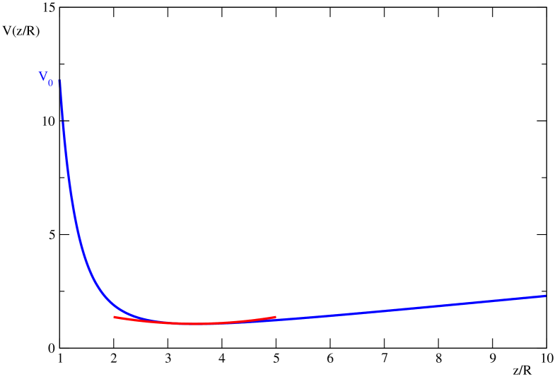
Figure 17: Blue line is the effective potential Eq. (A.13) for electrons drifting toward the stellar surface in the polar cup regions. The red line is the harmonic approximation to the potential.

In the case of minimal magnetic barrier, using Eq. (A.10) we rewrite Eq. (A.12) as:

$$V(z)\;\simeq\;11.6\;KeV\;B_{12}\;\frac{R^{3}}{z_{0}^{3}}\;\left[\left(\frac{z_{0}}{z}\right)^{3}\;-\;1\right]\;+\;0.23\;KeV\;n_{13}\;\frac{z}{R}\;,\;\;1\;\leq\;\frac{z}{R}\;\leq\;\frac{z_{0}}{R}\;\;,$$ (A.13)

where $n_{13}=\frac{n}{10^{13}\,cm^{-3}}\,$. In Fig. 17 we display the effective potential Eq. (A.13) assuming $z_{0}\simeq 10\,R$. We see that the effective potential $V(z)$ displays a minimum at $z=\bar{z}$ where the repulsive magnetic force is balanced by the attractive electric force. Then, electron are trapped above the polar cup at a distance of order $\bar{z}$. To determine the energy spectrum we need to solve the Schrödinger equation with the effective potential:

$$\frac{1}{2m_{e}}\left[-\frac{d^{2}}{dz^{2}}\;+\;V(z)\right]\zeta(z)\;=\;\varepsilon_{drift}\;\zeta(z)\;.$$ (A.14)

We may adopt the harmonic approximation to the potential by expanding around $\bar{z}$. A straightforward calculation gives:

$$\bar{z}\;\simeq\;3.5\;R\;B_{12}^{\frac{1}{4}}\;n_{13}^{-\frac{1}{4}}\;\;,\;\;\bar{V}\;\equiv\;V(\bar{z})\;\simeq\;1.08\;KeV\;B_{12}^{\frac{1}{4}}\;n_{13}^{\frac{3}{4}}\;\;\;.$$ (A.15)

Moreover:

$$R^{2}\;V^{{}^{\prime\prime}}(\bar{z})\simeq\;0.261\;KeV\;B_{12}^{-\frac{1}{4}}\;n_{13}^{\frac{5}{4}}\;\;\;.$$ (A.16)

Note that, as long as $z_{0}\gg R$, $\bar{z}$, $\bar{V}$ and $V^{{}^{\prime\prime}}(\bar{z})$ do not depend on $z_{0}$. In this approximation $\zeta(z)$ satisfies the harmonic oscillator equation centered at $\bar{z}$ with frequency:

$$\omega_{m}\simeq\;0.46\;10^{-12}\;eV\;B_{12}^{-\frac{1}{8}}\;n_{13}^{\frac{5}{8}}\;\;\;.$$ (A.17)

Thus, we find for the drift energy the quasi continuum spectrum:

$$\varepsilon_{drift,j}\;=\;\bar{V}\;+\;\omega_{m}\;(j\;+\;\frac{1}{2})\;\;,\;\;j\;\geq\;0\;\;\;.$$ (A.18)

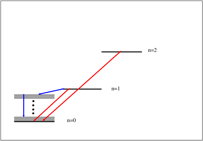
Figure 18: Energy spectrum for electrons trapped in the magnetosphere near the polar cups. Heavy lines are the Landau levels with cyclotron frequency $\omega_{B}$. Light lines are the quasi continuum spectrum Eq. (A.18). Red and blue arrows indicate possible radiative transitions.

Let us pause to briefly summarize our results. Our quantum mechanical treatment of charges which are drifting toward the star in the weakly varying dipolar magnetic field has shown that electrons feel a huge magnetic barrier. On the other hand, the magnetic barrier is reduced by a factor $\frac{m_{e}}{m_{p}}$ for protons. As a consequence, protons are free to reach the stellar surface, where they are trapped in the electron atmosphere, while electrons are repelled into the magnetosphere. The resulting charge separation produces an electric field which trapped electron at a distance $\sim\bar{z}$. Obviously, the neutrality of the plasma implies that the number densities of trapped electrons and protons are equal. The resulting picture is very interesting. We have electrons which oscillate around $\bar{z}$ along the magnetic field. On the other hand, these electrons feel the magnetic field $B(\bar{z})$, which now is truly almost constant. So that, if $\omega_{B}$ is the cyclotron frequency at $\bar{z}$, then using Eq. (A.15) we get:

$$\omega_{B}\;=\;\frac{eB(\bar{z})}{m_{e}}\simeq\;0.268\;KeV\;B_{12}^{\frac{1}{4}}\;n_{13}^{\frac{3}{4}}\;\;\;.$$ (A.19)

Then, the energy spectrum of these electrons is:

$$E_{n,j}\;=\;\bar{V}\;+\;\omega_{B}\;n\;+\;\omega_{m}\;(j\;+\;\frac{1}{2})\;\;,\;\;\;\;n\;,\;j\;\geq\;0\;\;\;.$$ (A.20)

In Figure 18 we illustrate schematically the spectrum Eq. (A.20). According to Eq. (A.20) the spectrum comprises discrete Landau levels with cyclotron frequency $\omega_{B}$ and an almost continuum associated to the drifting motion. As discussed below, electrons perform radiative transition between Landau levels. These transitions are responsible for absorption and spectral features observed in isolated $X$-ray pulsars, anomalous $X$-ray pulsars and soft gamma ray repeaters. Moreover, we see that there are also transitions where electrons absorb thermal photons with frequency $\omega\sim\omega_{B}$ and emit photons with frequencies $\omega^{{}^{\prime}}\ll\omega$. These radiative transitions give rise to the soft spectrum. Before addressing the problem of the soft spectrum, let us discuss the puzzling absorption features detected in the isolated $X$-ray pulsar 1E 1207.4-5209 [99]. The spectrum of 1E 1207.4-5209 shows three distinct features, regularly spaced at $0.7\;KeV$, $1.4\;KeV$ and $2.1\;KeV$, plus possibly a fourth at $2.1\;KeV$. These features vary in phase with the star rotation. Indeed, it turns out that the $X$-ray source pulsation is largely due to the phase variation of the lines with the pulsar rotation. The most natural and logical explanation for the observed features is cyclotron resonant absorption. In this case the fundamental cyclotron frequency is $0.7\;KeV$. Thus, the inferred magnetic field is $\sim 8\,10^{10}\;Gauss$ for electrons and $\sim 2\,10^{14}\;Gauss$ for protons. However, the magnetic field inferred from the spin parameters turns out to $B_{S}\simeq 2.4\,10^{12}\;Gauss$. Obviously, as noted in Ref. [99] electron cyclotron scattering at a distance $3-4\;R$ above the pulsar surface would fit all the observations. Remarkably, using the inferred magnetic field $B_{S}$ and Eq. (A.19) we find:

$$\omega_{B}\;\simeq\;0.7\;KeV\;\;,\;\;\;B_{S,12}\;\simeq\;2.4\;\;\;\;n_{13}\;\simeq\;2.69\;\;\;.$$ (A.21)

Moreover from Eq. (A.15) we get $\bar{z}\;\simeq\;3.4\;R$, in perfect accord with observations. Finally, we stress that the presence of the almost continuum spectrum associated to the drifting motion along the magnetic field leads naturally to rather broader spectral features in accord with several observations. Even though it is beyond the aim of the present Section an accurate comparison with available data, we would like to stress that our proposal is in gratifying qualitative agreement with observations. Indeed, absorption features have been found in the thermal emission of several isolated $X$-ray pulsars which range in $0.2-0.7\;KeV$. The thermal spectrum of isolated $X$-ray pulsar is a blackbody with typical temperature $T\sim 0.1KeV$. Now Eq. (A.19) shows that for typical pulsar magnetic field $B_{12}\sim 1$ the electrons trapped at $\sim\bar{z}$ are able to absorb thermal photons in the observed range. Note that for magnetars the typical blackbody temperature is $T\sim 1.0\;KeV$ (the relevant temperature is the polar cup blackbody temperature), and $B_{12}\sim 10^{2}$. So that Eq. (A.19) gives $\omega_{B}\;\sim\;0.85\;KeV$, indicating that also for magnetars the trapped electrons may efficiently absorb the thermal photons from the polar cups.
Let us discuss, now, the radiative transitions from trapped electrons. To evaluate the rate of transitions we need to evaluate:

$$\left|\frac{ie}{m_{e}}\;<n^{{}^{\prime}},j^{{}^{\prime}}|\;\exp(-i\vec{k}\cdot\vec{r})\;\vec{l}\cdot\vec{\nabla}\;|n,j>\right|^{2}\;\;\;,$$ (A.22)

where:

$$|n,j>\;=\;\zeta_{j}(z)\;\phi_{n}(x,y)\;\;\;,\;\;\vec{l}\cdot\vec{k}\;=\;0\;\;\;,$$ (A.23)

$\vec{k}$ and $\vec{l}$ being the photon momentum and polarization respectively. Without loss in generality, we may write:

$$\vec{k}\;=\;(k_{\bot},0,k_{3})\;\;\;,\;\;\;\vec{l}\;=\;(0,1,0)\;\;\;,$$ (A.24)

so that:

$$\left|\frac{ie}{m_{e}}\;<n^{{}^{\prime}},j^{{}^{\prime}}|\;\exp(-i\vec{k}\cdot\vec{r})\vec{l}\cdot\vec{\nabla}\;|n,j>\right|^{2}\;=\;\frac{e^{2}}{m_{e}^{2}}\;I_{n^{{}^{\prime}},n}\;J_{j^{{}^{\prime}},j}\;\;\;,$$ (A.25)

where:

$$I_{n^{{}^{\prime}},n}\;=\;\left|\;<n^{{}^{\prime}}|\;\exp(-ik_{\bot}x)\frac{\partial}{\partial y}\;|n>\right|^{2}\;\;\;\;,$$ (A.26)

$$J_{j^{{}^{\prime}},j}\;=\;\left|\;<j^{{}^{\prime}}|\;\exp(-ik_{3}z)\;|j>\right|^{2}\;\;\;\;.$$ (A.27)

Obviously we have also:

$$|\vec{k}|\;=\;E_{n^{{}^{\prime}},j^{{}^{\prime}}}\;-\;E_{n,j}\;=\;\omega_{B}\;(n^{{}^{\prime}}\;-\;n)\;+\;\omega_{m}\;(j^{{}^{\prime}}\;-\;j)\;\;\;.$$ (A.28)

We are interested in processes where trapped electrons absorb thermal photons with energy $\sim\omega_{B}$ (red lines in Fig 18) and emits photons with $|\vec{k}|\ll\omega_{B}$ (blue lines in Fig. 18). Since $\omega_{m}\sim 10^{-12}\;eV$, from Eq. (A.28) it follows that $\Delta j\gg 1$. Then, the transitions $j\rightarrow j^{{}^{\prime}}$ cannot be induced by the electromagnetic field. Indeed, these transitions are induced by thermal collisions. To see this, we note that for $j\gg 1$ the wave function $\zeta(z)$ is quasi classical:

$$\zeta(z)\;\sim\;\exp[-ip(z)z]\;\;\;,$$ (A.29)

where $p(z)$ is the quasi classical momentum. Now, Eq. (A.27) means that $J_{j^{{}^{\prime}},j}$ is different from zero if the momentum is conserved. However, for vastly different quasi momenta the overlap of the quasi classical wave function is very small. So that we are lead to the conclusion that $|k_{3}|\ll|k_{\bot}|$. As a consequence we see that the transitions must be induced by collisions, so that we may safely assume $|J_{j^{{}^{\prime}},j}|\simeq 1$. To evaluate $I_{n^{{}^{\prime}},n}$ we need the wave functions $\phi_{n}(x,y)$:

$$\phi_{n}(x,y)\;=\;\frac{\exp(-ip_{x}x)}{\sqrt{2\pi}}\;\sqrt{\frac{m_{e}\omega_{B}}{n!2^{n}}}\;\frac{1}{\pi^{\frac{1}{4}}}\;\exp[-\frac{m_{e}\omega_{B}}{2}(y-\frac{p_{x}}{m_{e}\omega_{B}})^{2}]\;\;H_{n}[\sqrt{m_{e}\omega_{B}}(y-\frac{p_{x}}{m_{e}\omega_{B}})]\;\;.$$ (A.30)

The most important transition is for $n^{{}^{\prime}}=1,n=0$. A standard calculations gives:

$$I_{1,0}\;=\;\frac{m_{e}\omega_{B}}{2}\;\left(1\;-\;\frac{k_{\bot}^{2}}{2m_{e}\omega_{B}}\right)^{2}\;\exp\left[-\frac{k_{\bot}^{2}}{2m_{e}\omega_{B}}\right]\;\;\;,$$ (A.31)

so that:

$$\left|\frac{ie}{m_{e}}\;<n^{{}^{\prime}},j^{{}^{\prime}}|\;\exp(-i\vec{k}\cdot\vec{r})\;\vec{l}\cdot\vec{\nabla}\;|n,j>\right|^{2}\;\simeq\;\frac{e^{2}\omega_{B}}{2m_{e}}\;\left(1\;-\;\frac{k_{\bot}^{2}}{2m_{e}\omega_{B}}\right)^{2}\;\exp\left[-\frac{k_{\bot}^{2}}{2m_{e}\omega_{B}}\right]\;.$$ (A.32)

Note that in our approximation $|\vec{k}|=k\simeq|k_{\bot}|\ll\omega_{B}$. Thus, we have:

$$\left|\mathcal{A}_{if}\right|^{2}\;\equiv\;\left|\frac{ie}{m_{e}}\;<n^{{}^{\prime}},j^{{}^{\prime}}|\;\exp(-i\vec{k}\cdot\vec{r})\;\vec{l}\cdot\vec{\nabla}\;|n,j>\right|^{2}\;\simeq\;\frac{e^{2}\omega_{B}}{2m_{e}}\;\;\;.$$ (A.33)

It is clear that Eq. (A.33) leads to a power law emission flux with the cutoff $k\ll\omega_{B}$. Moreover, to get the flux we need to assume some energy distribution for the trapped electrons, which, however, goes beyond the aim of the present paper. Nevertheless, there is a general aspect which is worthwhile to stress. We have seen that the soft spectrum in isolated pulsar can be understood as thermal photons reprocessed by electrons trapped in the magnetosphere above the polar cups. These electrons absorb thermal photons with frequency $\sim\;\omega_{B}$ and emit photons with frequencies $\ll\;\omega_{B}$. So that the number of these electrons is proportional to the number of thermal photons with energy $\sim\;\omega_{B}$. We know that $\omega_{B}\sim T$, where $T$ is the blackbody temperature. As a consequence, recalling that the number density of thermal photons scale as $\sim T^{3}$, we have that the soft fluxes in magnetars should be about a factor $(T_{magnetar}/T_{pulsar})^{3}\sim 10^{3}$ greater than the one in isolated $X$-ray pulsars, in fair agreement with observations.
Let us conclude this Appendix by roughly estimating the soft flux $F_{\omega}$. The probability for emission of a photon in the frequency range $\omega$, $\omega+d\omega$ is:

$$\frac{dP}{dt\;d\omega}\;=\;\frac{\omega}{2\pi}\;\left|\mathcal{A}_{if}\right|^{2}\;\delta[\omega\;-\;(E_{1,j^{{}^{\prime}}}\;-\;E_{0,j})]\;\;\;,$$ (A.34)

where we used $\omega=|\vec{k}|=k\simeq|k_{\bot}|$, and the delta function ensures the energy conservation Eq. (A.28). Summing over the degenerate final states of the almost continuum spectrum, and using $d\omega=\omega_{m}\;dj^{{}^{\prime}}$, we get:

$$\frac{dP}{dt\;d\omega}\;\simeq\;\frac{1}{2\pi}\;\frac{\omega}{\omega_{m}}\;\frac{e^{2}\omega_{B}}{2m_{e}}\;\;\;.$$ (A.35)

Finally, the spectral flux is obtained multiplying by the photon energy $\omega$ and by the number of active electrons. Let $n_{act}$ be the number density of active electrons, we have:

$$F_{\omega}\;\simeq\;\frac{1}{2\pi}\;\frac{\omega^{2}}{\omega_{m}}\;\frac{e^{2}\omega_{B}}{2m_{e}}\;n_{act}\;V\;\;,\;\;\;\omega\;\ll\;\omega_{B}\;\;\;,$$ (A.36)

where $V$ is the volume of the emitting region. Note that $F_{\omega}$ has a Rayleigh-Jeans power law form with an upper cutoff which, however, cannot be easily estimated without a precise knowledge of electron energy distribution. Using Eqs. (A.17) and (A.19), we rewrite Eq. (A.36) as:

$$F_{\omega}\;\simeq\;8.2\;10^{-6}\;\frac{ergs}{sec\;Hz}\;(\frac{\omega}{1eV})^{2}\;B_{12}^{\frac{3}{8}}\;n_{13}^{\frac{1}{8}}\;\;n_{act}\;V\;\;\;\;\;.$$ (A.37)

The number density of active electrons is not easily estimated without the knowledge of the energy distribution of electrons trapped into the magnetosphere. In general, $n_{act}$ depends on the number of thermal photons with energy $\omega\sim\omega_{B}$. Nevertheless, we may estimate the needed number density $n_{act}$ by comparing with observed soft fluxes. For typical isolated $X$-ray pulsar with $B_{12}\sim 1$ and $n_{13}\sim 1$ we infer:

$$F_{\omega}\;\simeq\;\;10^{13}\;\frac{ergs}{sec\;Hz}\;\;,\;\;\omega\;\simeq\;1eV\;\;.$$ (A.38)

So that, assuming for the emitting volume the reasonable value $V\,\sim\,10^{10}\;cm^{3}$, from Eq. (A.37) we get:

$$n_{act}\;\sim\;\;10^{8}\;cm^{-3}\;\sim\;10^{-5}\;n\;\;\;.$$ (A.39)

It is interesting to compare Eq. (A.39) with the number density of active electrons obtained assuming that trapped electrons have an uniform distribution. In this case, observing that the probability for transitions from the $n=0$ to $n=1$ Landau levels is given by Eq. (A.32) with $k_{\bot}\simeq\omega_{B}$, we get:

$$n_{act}\;\simeq\;\frac{e^{2}\omega_{B}}{2m_{e}}\;n\;\;\;.$$ (A.40)

So that, for typical isolated $X$-ray pulsars we have:

$$n_{act}\;\simeq\;2.4\;10^{-5}\;n\;\;\;,$$ (A.41)

that, indeed, is in reasonable agreement with our estimate Eq. (A.39).

References

- [1] A. Hewish, S. G. Bell, J. D. H. Pilkington, P. F. Scott, and R. A. Collins, Nature 217 (1968) 709 .
- [2] W. Baade and F. Zwicky, Proc. Nat. Acad. Sci. 20 (1934) 254 ; Phys. Rev. 45 (1934) 138 ; Phys. Rev. 46 (1934) 76.
- [3] F. Pacini, Nature 219 (1968) 145.
- [4] T. Gold, Nature 218 (1968) 731.
- [5] See, for instance: F. C. Michel, Rev. Mod. Phys. 54 (1982) 1; F. C. Michel, The State of Pulsar Theory , astro-ph/0308347.
- [6] F. C. Michel, Theory of Neutron Star Magnetospheres, (The University of Chicago Press, Chicago, 1991).
- [7] P. Goldreich and W. H. Julian, Astrophys. J. 157 (1969) 869.
- [8] P. A. Sturrock, Astrophys. J. 164 (1971) 529.
- [9] P. Cea, Int. J. Mod. Phys. D13 (2004) 1917.
- [10] P. Cea, JCAP 0403011 (2004).
- [11] For a review, see: H. A. Bethe, Rev. Mod. Phys. 62 (1990) 801.
- [12] M. R. Gargcia, J. E. McClintock, R. Narayan, P. Callanan, and S. S. Murray, Astrophys. J. 553 (2001) L47.
- [13] S. Campana and L. Stella, Astrophys. J. 541 (2000) 849 .
- [14] S. L. Robertson and D. J. Leiter, Astrophys. J. 565 (2002) 447 .
- [15] For instance, see: J. Frank, A. King, and D. Raine, Accretion Power in Astrophysics, (Cambridge University Press, Cambridge, 2002).
- [16] S. L. Robertson and D. J. Leiter, Mon. Not. Roy. Astron. Soc. 350 (2004) 1391.
- [17] S. L. Robertson and D. J. Leiter, Astrophys. J. 596 (2003) L203 .
- [18] D. J. Leiter and S. L. Robertson , Found. Phys. Lett. 16 (2003) 143 .
- [19] For a review see: F. Melia and H. Falcke, Ann. Rev. Astron. Astroph. 39 (2001) 309.
- [20] F. K. Baganoff et al., Astrophys. J. 591 (2003) 891
- [21] M. P. Muno et al., Diffuse X-ray Emission in a Deep Chandra Image of the Galactic Center, astro-ph/0402087.
- [22] S. Nayakshin, Using close stars as probes of hot accretion flow in Sgr A*, astro-ph/0410455.
- [23] J.-H. Zhao, G. C. Bower, and W. M. Goss, Astrophys. J. 547 (2001) L29.
- [24] A. Miyazaki, t. Tsutsumi, and M. Tsuboi, Astron. Nachr. Suppl. 324 (2003) 363.
- [25] F. Haberl, AXPs and X-ray dim neutron stars: Recent XMM-Newton and Chandra results, astro-ph/0302540.
- [26] G. G. Pavlov and V. E. Zavlin, Proceedings 21st Texas Symposium on Relativistic Astrophysics, Edited by R. Bandiera, R. Maiolino and F. Mannucci, Singapore, World Scientific, 2003, pag. 319.
- [27] V. Burwitz, F. Haberl, R. Neuhäuser, P. Predehl, J. Trümper, and V. E. Zavlin, Astron. Astrophys. 399 (2003) 1109 .
- [28] D. Kaplan, Optical Observations of Isolated Neutron Stars, contribute to the workshop Physics and Astrophysics of Neutron Stars, July 28 - August 1, 2003, Santa Fe, New Mexico.
- [29] X.-D. Li, Z. G. Dai, and Z.-R. Wang, Astron. Astrophys. 303 (1995) L1.
- [30] See, for insatnce: S. L. Shapiro and S. A. Teukolsky, Black Holes, White Dwarfs, and Neutron Stars, (John Wiley & Sons , 1983).
- [31] A. P. Reynolds, P. Roche, and H. Quaintrell, Astron. Astrophys. 317 (1997) L25.
- [32] S. M. Ransom, J. W. T. Hessels, I. H. Stairs, P. C. C. Freire, F. Camilo, V. M. Kaspi and D. L. Kaplan, Twenty-One Millisecond Pulsars in Terzan 5 Using the Green Bank Telescope, astro-ph/0501230.
- [33] O. Barziv et al., Astron. Astrophys. 377 (2001) 925.
- [34] H. Quaintrell et al., Astron. Astrophys. 401 (2003) 313.
- [35] S. Mereghetti, The Anomalous -ray Pulsars, astro-ph/9911252.
- [36] S. Mereghetti, L. Chiarlone, G. L. Israel, and L. Stella, The Anomalous -ray Pulsars, astro-ph/0205122.
- [37] V. M. Kaspi and F. P. Gavriil, Nucl. Phys. Proc. Suppl. 132 (2004) 456.
- [38] K. Hurley, The 4.5 0.5 Soft Gamma Repeaters in Review, astro-ph/9912061.
- [39] P. M. Woods, The Dynamic Behavior of Soft Gamma Repeaters, astro-ph/0304372.
- [40] V. M. Kaspi, Soft Gamma Repeaters and Anomalous -ray Pulsars: Together Forever, astro-ph/0402175.
- [41] P. M. Woods and C. Thompson, Soft Gamma Repeaters and Anomalous -ray Pulsars: Magnetar Candidates, astro-ph/0406133.
- [42] R. C. Duncan and C. Thompson, Astrophys. J. 392 (1992) L9.
- [43] B. Paczyński, Acta Astron. 42 (1992) 145.
- [44] R. C. Duncan and C. Thompson, Mon. Not. Astron. Soc. 275 (1995) 255.
- [45] R. C. Duncan and C. Thompson, Astrophys. J. 473 (1996) 322.
- [46] R. C. Duncan and C. Thompson, Astrophys. J. 408 (1993) 194.
- [47] M. Chaichian, S. S. Masood, C. Montonen, A. Perez Martinez and H. Perez Rojas, Phys. Rev. Lett. 84 (2000) 5261.
- [48] R. N. Manchester and J. H. Taylor, Pulsars, (W. H. Freeman and Company, San Francisco, 1977).
- [49] http://www.atnf.csiro.au/research/pulsar/psrcat.
- [50] P. Cea, On the Pulsar Emission Mechanism, astro-ph/0403568.
- [51] M. Burgay et al., Nature 426 (2003) 531.
- [52] A. G. Lyne et al., Science 303 (2004) 1153.
- [53] M. A. McLaughlin et al., Astrophys. J. 613 (2004) L57.
- [54] M. G. Baring and A. K. Harding, Astrophys. J. 507 (1998) L55.
- [55] G. Hobbs et al., Mon. Not. Astron. Soc. 352 (2004) 1439.
- [56] M. A. McLaughlin et al., Astrophys. J. 591 (2003) L135.
- [57] M. Cropper, F. Haberl, S. Zane, and V. E. Zavlin, Mon. Not. Roy. Astron. Soc. 351 (2004) 1099.
- [58] B. Cheng, R. I, Epstein, R. A. Guyer, and A. Cody Young, Nature 382 (1995) 518.
- [59] K. J. Hurley, B. McBreen, M. Rabbette, and S. Steel, Astron. Astrophys. 288 (1994) L49.
- [60] P. M. Woods et al., Astrophys. J. 605 (2004) 378.
- [61] P. M. Woods et al., Astrophys. J. 524 (1999) L55.
- [62] C. Thompson, R. C. Duncan, P. M. Woods, C. Kouveliotou, M. H. Finger, and J. Van Paradijs, Astrophys. J. 543 (2000) 340.
- [63] S. Mereghetti et al., A XMM-Newton View of the Soft Gamma-ray Repeater SGR 1806–20: Long Term Variability in the pre-Super Giant Flare Epoch, astro-ph/0502417.
- [64] K. A. Van Riper, Astrophys. J. 372 (1991) 251.
- [65] E. H. Gundmundsson, C. J. Pethick, and R. I. Epstein, Astrophys. J. 272 (1983) 286.
- [66] D. Marsden and N. E. White, Astrophys. J. 551 (2001) L155.
- [67] M. Morii et al., Publ. Astr. Soc. Japan 55 (2003) L45.
- [68] F. Özel, Astrophys. J. 575 (2002) 397.
- [69] See, for instance: W. H. Wallace, Radiation Processes in Astrophysics (MIT Press, Cambridge, 1977); V. L. Ginzburg, Theoretical Physics and Astrophysics (Pergamon, Oxford, 1979).
- [70] D. A. Frail, S. R, Kulkarni, and J. S. Bloom, Nature 398 (1999) 127.
- [71] B. M. Gaensler et al., An expanding radio nebula produced by a giant flare from the magnetar SGR 1806-20, astro-ph/0502393.
- [72] P. B. Cameron et al., Discovery of a Radio Afterglow following the 27 December 2004 Giant Flare from SGR 1806-20, astro-ph/0502428.
- [73] X. Y. Wang, X. F. Wu, Y. Z. Fan, Z. G. Dai, and B. Zhang, An energetic blast wave from the December 27 giant flare of the soft gamma-ray repeater 1806-20, astro-ph/0502085.
- [74] J. Granot et al., Diagnosing the outflow from the SGR 1806-20 Giant Flare with Radio Observations, astro-ph/0503251.
- [75] J. D. Gelfand et al., A Re-brightening of the Radio Nebula associated with the 2004 December 27 giant flare from SGR 1806–20, astro-ph/0503269.
- [76] J. Schwinger, Phys. Rev. 75 (1949) 1912 .
- [77] See, for instance: P. J. E. Peebles, Principles of Physical Cosmology, (Princeton University Press, Princeton, New Jersey, 1993).
- [78] C. Alcock, E. Farhi, and A. V. Olinto, Astrophys. J. 310 (1986) 261.
- [79] M. Feroci et al., Astrophys. J. 515 (1999) L9.
- [80] K. Hurley et al., A tremendous flare from SGR1806-20 with implications for short-duration gamma-ray bursts, astro-ph/0502329.
- [81] M. Feroci, K. Hurley, R. C. Duncan, and C. Thompson, Astrophys. J. 549 (2001) 1021.
- [82] D. Götz, S. Mereghetti, I. F. Mirabel, and K. Hurley, Astron. Astrophys. 417 (2004) L45.
- [83] R. C. Duncan and C. Thompson, Astrophys. J. 561 (2001) 980.
- [84] Y. Lyubarski, D. Eichler, and C. Thompson, Astrophys. J. 580 (2002) L69.
- [85] C. R. Tam, V. M. Kaspi, M. H. van Kerkwijk and M. Durant, Correlated Infrared and X-ray Flux Changes Following the 2002 June Outburst of the Anomalous X-ray Pulsar 1E 2259+586, astro-ph/0409351.
- [86] A. I. Ibrahim et al., Astrophys. J. 558 (2001) 237.
- [87] K. Hurley et al., Astrophys. J. 510 (1999) L111.
- [88] P. M. Woods et al., Astrophys. J. 552 (2001) 748.
- [89] M. Feroci et al., Astrophys. J. 596 (2003) 470.
- [90] G. T. Lenters et al., Astrophys. J. 587 (2003) 761.
- [91] J. F. Olive, J. L. Atteia, K. Hurley, G. Crew, G. Ricker, and G. Pizzichini, Time-resolved X-ray spectral modeling of an intermediate burst from SGR1900+14 observed by HETE-2/FREGATE, astro-ph/0403162.
- [92] C. Kouveliotou, M. Kippen, P. Woods, G. Richardson, V. Connaughton, and M. McCollough, IAU Circ. 6944, 1998.
- [93] P. M. Woods et al., Astrophys. J. 519 (1999) L139
- [94] C. Kouveliotou et al., Astrophys. J. 596 (2003) L79.
- [95] S. Mereghetti, D. Götz, A. von Kienlin, A. Rau, G. Lichti, G. Weidenspointner, and P. Jean, The first giant flare from SGR 1806-20: observations with the INTEGRAL SPI Anti-Coincidence Shield, astro-ph/0502577.
- [96] P. Cea and L. Cosmai, Nucl. Phys. Proc. Suppl. 119 (2003) 700.
- [97] P. Cea and L. Cosmai, JHEP02 (2003) 031.
- [98] G. Israel et al., Unveiling the multi-wavelength phenomenology of Anomalous X-ray Pulsars, astro-ph/0310482.
- [99] G. F. Bignami, P. A. Caraveo, A. De Luca, and S. Mereghetti, Nature 423 (2003) 725.