Applying Machine Learning to Catalogue Matching in Astrophysics

Abstract

We present the results of applying automated machine learning techniques to the problem of matching different object catalogues in astrophysics. In this study we take two partially matched catalogues where one of the two catalogues has a large positional uncertainty. The two catalogues we used here were taken from the HI Parkes All Sky Survey (HIPASS), and SuperCOSMOS optical survey. Previous work had matched $44\%$ ($1887$ objects) of HIPASS to the SuperCOSMOS catalogue.

A supervised learning algorithm was then applied to construct a model of the matched portion of our catalogue. Validation of the model shows that we achieved a good classification performance ($99.12\%$ correct).

Applying this model, to the unmatched portion of the catalogue found $1209$ new matches. This increases the catalogue size from $1887$ matched objects to $3096$. The combination of these procedures yields a catalogue that is $72\%$ matched.

1 Introduction

The Virtual Observatory will bring new opportunities and new challenges. Our study works with a problem that may become typical in the virtual observatory context: the problem of matching catalogues with significant positional uncertainties.

The Virtual Observatory will allow efficient access to the vast amounts of data being collected by all sky surveys in many wavelengths. A fundamental operation for increasing the utility of this data will be the matching of catalogues. Matching catalogues will utilise many components of the virtual observatory. The main task of these services will be to perform a fuzzy (probabilistic) distributed spatial join. Distributed computing is required so that catalogues can be published at appropriate sites all over the world. Special indexes have also been developed to aid in doing fast spatial joins; at present Open SkyQuery (Budavári et al., 2004) is leading progress toward making this a reality. The study reported in this paper is focused on the fuzzy or probabilistic component of this problem. That is, for a given source, how is the correct counterpart chosen out of a number of candidate matches within the error ellipse? Supervised learning techniques have already been applied to the astronomy problems of star-galaxy classification (Bertin & Arnout, 1996; Andreon et al., 2000), galaxy morphology classification (Bazell & Aha, 2001) and the search for quasars in photometric data (Richards et al., 2001). A review paper of astronomical applications in machine learning can be found in Tagliaferri et al. (2003). Both within astronomy and in other applications the focus of supervised learning techniques is on regression or pattern classification. The specific type of pattern classification problem (the matching problem) which we consider here is reasonably novel and the authors believe warrants further attention. A related, but underdeveloped field in computer science is the problem of record linkage (Fellegi & Sunter, 1969). The solution to the problem of matching catalogues is likely to have an impact on record linkage, which demonstrates just one way that the development of the virtual observatory may impact on fields outside astronomy. Borrowing from computer science this paper uses the term linkage to refer to the problem of resolving the ambiguity in the matching problem. We draw the distinction between this problem and the computational and network problems associated with matching catalogues. The database term of joining suggests itself as being appropriate for describing catalogue matching problems focused on the computational or distributed nature of the problem. In this paper we focus on the problem of linkage.

A number of simple approaches to linkage are commonly used in astronomy. Often taking the closest match (in terms of position only) is considered adequate especially when the positional uncertainties are small, for example Drinkwater et al. (1997) (positional uncertainties are of the order of arcseconds). Another more sophisticated technique, the likelihood ratio, compares the probability that the object is a match in comparison to the probability that it is a chance background object (Sutherland & Saunders, 1992). The likelihood ratio itself only utilises a small number of parameters (and only those from the more dense catalogue).

Our work uses supervised learning techniques from machine learning in order to link these two catalogues using all available information. Our overall goal is to provide a proof of concept that the full parameter list (or an intelligently chosen subset) contains useful information that can be used to reliably link catalogues. While a simple method of performing linkage using a simple supervised learning algorithm (decision trees) has been previously demonstrated by Voisin & Donas (2001), no follow up work on the topic has been published. This study offers a more complete treatment of the problem in a number of ways. External information is used to construct the training set; Voisin and Donas simply used a cut on proximity to assign labels. We also analyse the scientific implications of different matching algorithms and investiage different and arguably more powerful algorithms.

The linkage method we propose is well suited to a certain class of problem. First of all there must be a significant linkage problem; the positional uncertainty of one catalogue must be large enough that there are frequently multiple candidate links in the more dense catalogue. This method also requires that there is a minimum and maximum amount of information available. There must be a significant subset of the catalogues that is already linked; this is vital for us to pursue a supervised learning procedure. It is also important that a significant subset of the catalogue remains unlinked in order for the procedure to cause a significant increase in the catalogue size.

The problem we discuss here involves joining a catalogue with comparatively poor positional uncertainties (HICAT, Meyer et al. (2004)) to a catalogue with good positional uncertainties (SuperCOSMOS, Hambly et al. (2001)). In general the positional resolution of the survey affects both the positional uncertainties and the density of sources per unit area of sky. In this study the SuperCOSMOS catalogue is the more dense catalogue and HICAT is the sparse catalogue. A general statement of our problem is for each object in the sparse catalogue to choose the correct counterpart from the dense catalogue. While it is not guaranteed that there is a single link in the dense catalogue, we are only dealing with the cases where we assume this to be true.

In this paper, we extend the work previously presented in Rohde et al. (2004) by considering the output (new matches) of the matching procedure that we have developed. This work is also applied to the final version of the HOPCAT Catalogue.

This paper has the following structure. Section 2 discusses the problem domain that we are investigating (in particular the catalogues involved). Section 3 discusses the construction and validation of the model. Section 4 discusses how we apply the model to the unmatched portion of the HIPASS Optical Catalogue (HOPCAT) in order to match a further $1209$ objects. Section 5 concludes by making some overall comments about our results.

2 Problem Domain and Catalogue Details

2.1 HICAT

The HI Parkes All Sky Survey (HIPASS) is a survey of the entire southern sky for HI. The HIPASS catalogue (HICAT) (Meyer et al., 2004) was produced by signal processing software run over the HIPASS data cubes. The result of this catalogue is 4315 HI sources with accurate redshifts and significant positional uncertainties where (RA has a $\sigma=0.78$ arcminutes (Zwaan et al., 2004)). HICAT describes each source using many parameters, the most important of these are velocity, peak flux ($S_{p}$), integrated flux ($S_{int}$) and velocity width.

2.2 SuperCOSMOS

SuperCOSMOS is a survey of the entire southern sky on photographic plates taken by the UK Schmidt Telescope. This is imaging data and as such has accurate positions but no redshift.

A catalogue has been produced of the SuperCOSMOS Images, the description of the image processing used to extract this catalogue is described in Hambly et al. (2001). For this application it was decided that it was best to reprocess the images using the SExtractor package (Bertin & Arnout, 1996) to obtain better segmentation. The SuperCOSMOS parameters are area, semi-major axis, semi-minor axis, $B_{j}$ (mag), $R$ (mag) and $I$ (mag). This catalogue contained a large number of stars which obviously were non-matching, for this reason it was decided to also provide a star-galaxy classification. SExtractor can only provide star-galaxy separation using its built in neural network when the images are from a CCD rather than a photographic plate. For this reason the following two step procedure was used to obtain classes. Diffraction spikes were observed as an obvious feature to assist in star-galaxy classification. Software was written using the cfitsio library which analysed the images and measured the length of the spikes of all objects. A training set was then constructed of $1000$ galaxies and $1000$ stars and a support vector machine(see Section 3.3) was trained to classify these objects using all of the previously mentioned SuperCOSMOS features as well as the diffraction spike feature. The use of machine learning techniques have been common place for the problem of star-galaxy classification for some time (Tagliaferri et al., 2003; Bertin & Arnout, 1996). Using a cross validation methodology where the algorithm is tested on data that it was not trained on the star-galaxy classifier was able to show a performance of 88%.

2.3 HOPCAT

A complementary study by Doyle et al. (2004) produced the HOPCAT catalogue, which matched 1887 of the 4315 HICAT sources. The procedure for matching involved joining the optical candidates to redshift observations taken from the Six Degree Field survey (6dF) (Wakamatsu et al., 2003) and the NASA Extragalactic Database (NED). If all of the optical candidates had redshift information and if there was exactly one object matching the HICAT redshift then it was deemed to be a match. Please see (Doyle et al., 2004) for more details.

This procedure allowed the matching of many HICAT sources to optical counterparts. It is however a slow procedure requiring heavy human intervention and it also was inconclusive in cases where there was no additional redshift information from 6dF or NED.

3 Construction and Validation of Model

While supervised learning algorithms automate much of the model construction process, human judgment must be used at a number of steps. The choice of input variables must be made for the algorithm, this procedure is known as feature selection. There is no correct procedure for doing this, except to call upon human judgment. Learning algorithm performance is generally improved by the choice of a small but informative set of features.

Closely related to feature selection is the preprocessing of input variables. For example is it advantageous to provide raw magnitudes or colour index information? If the distribution of a variable is not uniform it may be advantageous to transform it prior to learning.

In this study a number of algorithms will be attempted and a procedure known as 10-fold cross validation is used to estimate the generalisation performance of these models (see Section 3.3). The best of these models is selected and performance is reported.

3.1 Feature Selection

In order for an optical parameter to be useful it must convey some useful information, either a relation between the optical parameter and radio parameters or something that will identify that the object is a galaxy likely to be a strong HI source. In contrast a radio parameter is only useful if it can be used to identify a relation between radio and optical parameters. The asymmetry above is due to the fact that there are many optical candidate matches for a single radio object.

In machine learning the parameters that are selected to build a model are called features. The rationale for our choice of features is as follows: log area and $B_{j}$ (mag) should be roughly correlated with log peak flux ($S_{p}$) and log integrated flux ($S_{int}$). Velocity is also a measure of distance so an inversely proportional relationship would be expected between velocity and either area or magnitude. We would expect highly elliptical optical objects to link with radio objects with high velocity widths. It was unclear if galaxy colour would contribute to the classifier, although it may be a means of detecting late-type galaxies that are likely to contain significant amounts of HI.

The only parameter not mentioned is separation, this is obviously useful as we would expect objects with low separation to be more likely to be matches.

The logarithm was taken of integrated flux, peak flux and area so that these would all roughly correlate with magnitude. A list of all the features selected as machine learning inputs is given in Table 1.

Feature	Origin	Name
1	Radio-Optical	Separation
2	Radio	Velocity
3	Radio	Velocity Width
4	Radio	Log Integrated Flux ($S_{int}$)
5	Radio	Log Peak Flux ($S_{p}$)
6	Optical	Log Isophotal Area
7	Optical	Semi-major Axis
8	Optical	Semi-minor Axis
9	Optical	$B_{j}$ (Magnitude)
10	Optical	$B_{j}-R$
11	Optical	$B_{j}-I$
12	Optical	Star-Galaxy classification

Table 1: Selected Features for machine learning inputs

3.2 Framing the Matching Problem as a Pattern Classification Problem

The matching problem is not framed automatically as a pattern classification problem. In order to make it one we combine inputs of radio and optical objects into a single vector. If the pair of objects are matching then the vector gets a positive label, otherwise the pair is given a negative label. The negative training points are determined by taking all the non-matching objects from the dense catalogue and pairing them with the respective object in the sparse catalogue. We also employ a mismatched set of negative examples which is discussed later.

It is normal to report the error on both the negative and the positive parts of the training set separately. This is particularly helpful in situations where the amount of positive and negative training data is unbalanced (we have $6.3$ negative examples for every positive). If a classifier was to always give a negative response it would trivially give a classification of $\frac{6.3}{7.3}$ or $86\%$ over all examples: $0\%$ on the positive data and 100% on the negative. For this reason the performance on the positive and negative data is reported separately. In order to avoid the inclusion of massive numbers of small and faint objects, only objects with an area greater than $600$ pixels were included in this study.

Here we report success rates rather than error rates. Error rates over the negative data are known as false positives and error rates over the positive data are known as false negatives. False positives and false negatives are related to traditional measures of completeness and efficiency. Both completeness and false negatives refer to the objects that are lost from the sample due to misclassification. Likewise efficiency and false positives refer to the incorrect objects that are found in our sample.

In this situation the relationships between completeness and false negatives, and efficiency and false positives are complicated by the framing of the problem in terms of binary pattern classification. In this situation the classifier is not constrained to give exactly one match; the ‘combinatorial’ nature of the output causes there to be no direct relationship between completeness and false negatives and efficiency and false positives.

3.3 Model Selection

There are a number of supervised learning algorithms that are appropriate to apply to this problem. One is the Support Vector Machine. The Support Vector Machine (SVM) computes a nonlinear mapping that transforms its input data into a high dimensional feature space where patterns of different classes can be separated by a hyperplane (Vapnik, 1995). The software being used is SVM Light (Joachims, 1998); this software is free for scientific use. SVMs have a number of parameters that can be tuned for optimal performance, including the kernel function. Kernel functions map the data to a high dimensional feature space. The SVM searches for a function that is linear in this high dimensional space, but non-linear in input space to separate these two classes. Popular kernels include linear, polynomial and radial basis functions (RBF) (Schölkopf & Smola, 2002).

SVMs also allow the soft margin (Cristianini & Shawe-Taylor, 2000) to be adjusted which is a parameter that controls the trade off between smooth and overly complex functions. Controlling this trade off is necessary to obtain good generalization. Functions that represent the training data well but do not generalise to novel examples are said to have overfit the data in machine learning terminology. The soft margin is a tool for the SVM to avoid overfitting.

Another popular and older algorithm is the neural network (Bishop, 1995). Neural networks are functions with a network-like topology and many free parameters. A gradient descent optimisation algorithm is used to partially search the parameter space for a suitable representation of the data. There are a countless number of heuristics for improving or altering the performance of neural networks, however in this study we implement the simplest of these algorithms i.e. backpropagation. The neural network is used with $3$, $4$, $5$ and $6$ hidden units. A neural network without any hidden units (the perceptron) is also used.

There is no way to know a priori which algorithm will give the best performance. The recommended procedure is to run a battery of tests using a good selection of candidate algorithms and parameters and measure the generalisation ability of each. An effective method for getting an accurate measure of generalisation ability is the 10-fold test. This involves dividing the training data into 10 equal parts, an algorithms is then trained on 9 of the subsets and tested on the 10th. This procedure is repeated 10 times in order to average this result over the entire dataset. The model which gave the best generalisation should then be selected. This procedure is known as cross validation. Table  1 shows the generalisation performance of multiple learning algorithms with different parameters. The SVM has different kernels (linear, polynomial and RBF) and different soft margins ($0.1$, $1$ and $10$). The neural networks have different number of hidden units (free parameters). Each network was trained for $1000$ iterations (“epochs”).

Table 2: Performance of Algorithms and parameters

Algorithm	Soft Margin	Pos Data	Neg Data	Overall
(Kernel)	(c) / hu	% correct	% correct	% correct
SVM	0.1	87.47 $\pm$2.24	98.70 $\pm$0.27	97.17
Linear	1	88.94 $\pm$2.43	98.75 $\pm$0.50	97.41
	10	88.80 $\pm$2.44	98.80 $\pm$0.25	97.43
SVM	0.1	90.04 $\pm$0.31	99.04 $\pm$1.67	97.93
Poly	1	94.18 $\pm$1.91	99.44 $\pm$0.20	98.72
d=2	10	96.02 $\pm$1.47	99.53 $\pm$0.29	99.05
SVM	0.1	94.91 $\pm$1.93	99.46 $\pm$0.27	98.84
Poly	1	96.24 $\pm$1.83	99.54 $\pm$0.20	99.09
d=3	10	96.69 $\pm$1.26	99.50 $\pm$0.42	99.12 *
SVM	0.1	89.39 $\pm$2.58	99.21 $\pm$0.27	97.87
RBF	1	93.66 $\pm$2.47	99.50 $\pm$0.28	98.70
$\gamma=1$	10	95.43 $\pm$1.69	99.66 $\pm$0.17	99.08
Perceptron		86.81 $\pm$7.73	97.52 $\pm$2.78	96.05
Neural Net	hu=3	93.81 $\pm$1.68	95.50 $\pm$1.41	95.27
	hu=4	94.10 $\pm$2.07	95.46 $\pm$1.38	95.27
	hu=5	93.50 $\pm$3.59	95.48 $\pm$1.26	95.21
	hu=6	93.45 $\pm$2.01	95.62 $\pm$1.23	95.32

Note: The errors reported are the standard deviation on the performance rate found when doing a 10-fold test. The asterisk (*) denotes the model with the best overall performance. The overall result takes in to account that there is approximately $6.3$ times as much negative data as positive, this results in more importance being required on classifying negative data correctly. The overall percentage correct is given by the formula : $R_{overall}=0.1365\times R_{pos}+0.8635\times R_{neg}$

In the second column, hu refers to hidden units in a neural network.

3.4 Model Performance

Running a battery of different algorithms showed that a SVM with a third degree polynomial and a soft margin of 10 was optimal (see Table  2). The percentages reported here are the result of 10-fold tests reported separately over positive and negative examples. This is useful, because sometimes the performance over the dataset and the performance over the positives and negatives vary considerably. Performance (in terms of percentage correct) over the positive and negative examples are reported separately. As the correctly classified examples (true positives and true negatives) are in all cases distributed over positives and negative data we can say that in all cases non-trivial models are found.

3.5 Feature Importance

Feature importance is the determination of how much information is given by each input. Feature importance is notoriously difficult (Guyon & Elisseeff, 2003). The reason for this is that in different combinations features have different effects, so in reality importance is a combinatorial problem. In the case of a matching problem the combinatorial nature is emphasised because inputs are of interest in the amount that they correlate with other inputs.

The measuring of the importance of the input is also highly tied to the problem of estimating the classification model. Adding features can make the estimation more difficult due to the curse of dimensionality . This has the potential to make the addition of useful features reduce overall classification performance.

The construction of our learning problem leads to some unusual characteristics. The positive learning vectors consist of variables from the sparse catalogue and the dense catalogue joined together. This means that the information from the sparse catalogue is repeated for every entry candidate match in the dense catalogue. Simulations on input importance have shown that optical parameters alone are often sufficient to achieve moderate classification. In this case we obtain a classification of 94%. At the outset of this project it was hoped that there would exist relationships between the radio and optical parameters which would aid in classification. This simulation shows that apriori, rejection of objects (stars and galaxies) from the dense catalogue is a more powerful element of this problem.

A special mismatched dataset was introduced to test the hypothesis that radio data could contribute any useful information. The dataset consisted of the normal positive matches, plus a random sample of radio sources matched to distant optical sources. The separation feature was removed from this simulation. Without radio information on this dataset 47% classification was achieved, while when radio information was added classification improved to 72%. This confirmed that relationships do exist between the radio and optical parameters of these galaxies.

4 Application of the Model to Unmatched Data

     

      (a)                    (b)                    (c)

     

      (d)                    (e)                    (f)

     

      (g)                    (h)                    (i)

Figure 1: A sample of the new matching objects

     

      (a)                    (b)                    (c)

     

      (d)                    (e)                    (f)

     

      (g)                    (h)                    (i)

Figure 2: Misclassified objects. a), b) are spurious ellipses marked as matches. c) d) and e) optical measurements of the velocities of the galaxies show that machine learning chose the wrong galaxy. f) g) and h) machine learning disagrees with HOPCAT, but there is insufficient information to establish which is correct. i) a bright star at close proximity is chosen as a match.

In order to apply our binary classification model to a HICAT source it must be evaluated against every candidate match in the HICAT region of uncertainty. This increases the chance of error from the above estimate because many model evaluations are required. There is also the chance that the classifier will find no matches, a single match or multiple matches. The performance measures given previously were for binary classification problems. The statistics of false positives and false negatives are highly related to, but are not measures of completeness and efficiency.

In order to see how well our model applies to the actual problem we examine only the unique velocity matches and test what agreement level this has with the HOPCAT catalogue. We take only the $1608$ unique velocity matches, out of $1887$ (this has an immediate bearing on the completeness of the catalogue). A sample of images of newly matching objects is shown in Fig  1. Of the 1608 only 9 are misclassified, indicating that the catalogue has high efficiency.

Accurate estimates of completeness and efficiency are not possible in this case for three reasons. The training data, and the data to which we apply the model have slightly different distributions. Our classifier output is a binary output over each output, allowing for ambiguous situations such as multiple matches to exist. A cross validation method (taking in to account unique matches) should be applied to produce this estimate. Finally we do not know how accurate the labels on our training data are (HOPCAT).

By ignoring cases of multiple matches we are able to sacrifice completeness for efficiency. We only get a false match when there are exactly two matches (one false positive and one false negative). This provides a level of error checking and means that the classifier is not applied to the difficult or ambiguous examples.

It is noteworthy that an error here requires exactly two errors over all the candidates and one of these must be on the match. The 9 misclassified objects are shown in Fig  2. This provides a form of error checking as if there are multiple matches then the chance that either the classifier has failed or that the match is ambiguous is high. A sample of images correctly classified are shown in Fig  1 and the 9 images incorrectly classified are shown in Fig  2.

HOPCAT contained 2221 objects which had insufficient information to match. It is this data that we wish to extract new information from, by matching it using machine learning.

The machine learning model found $1209$ of these were assigned unique matches by the model. The high accuracy on the test set suggests that a very high proportion of these matches are correct.

A plot of radio flux against optical magnitude of the old and new points is shown in Fig  3. The new data points appear to follow the same trend as the old data points. Although it is obvious that the two distributions are different: the new points are more likely to be fainter in both the optical and radio flux. This is most likely due to a selection effect where the training data contains brighter objects. It appears that the model is successfully extrapolating to fainter objects than the training data. The authors would like to stress that the quality of the machine learning model should be judged on the cross-validation performance, not the good agreement found here.

The SuperCOSMOS catalogue goes deeper than HICAT. The non-linear detection limits on HICAT can be seen in the distribution of integrated flux ($S_{int}$) Fig  4 and peak flux ($S_{p}$) Fig  5. The effect of this threshold is that objects with an $S_{int}$ $<0.5JyKms^{-1}$ are under represented in Fig  3, while the limit on optical magnitude is low enough to have negligible effect. This may be responsible for a subtle curve upwards for the faint end of the spectrum in Fig 3.

Over the $216$ blank fields $6(3\%)$ had one or more match on them. This gives a rough indication of the frequency of false positives.

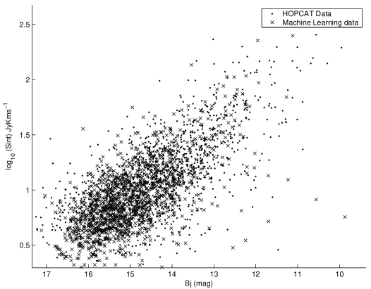
Figure 3: Magnitude Flux plot of old and newly obtained datapoints

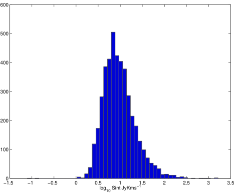
Figure 4: Distribution of integrated flux ($S_{int}$)

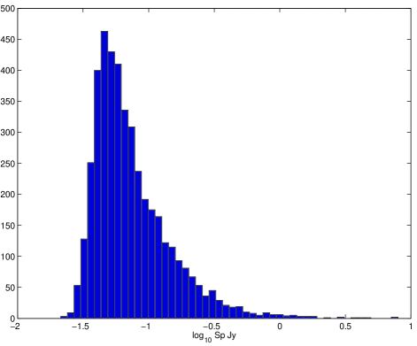
Figure 5: Distribution of peak flux ($S_{p}$)

5 Discussion

The matching of catalogues can be framed as a supervised learning, pattern classification problem. Despite differences between matching and pattern classification the algorithms performed remarkably well on this data, showing performance over $99\%$. The model we found produced the most discriminating power from the optical (dense) catalogue, however we were able to show that important relations existed between the two catalogues.

This method was successful in generating $1209$ new matches to the HOPCAT Catalogue, bringing the total number of matches to $3096$ out of $4315$. For a significant portion of the HICAT sources it is difficult or impossible to find a match because there are many optical counterparts; or the optical counterparts are obscured by the zone of avoidance.

The quality of both the source of the training data (HOPCAT) and the additional counterparts found using machine learning, need to be verified using high resolution radio data from the Australian Telescope Compact Array. Verification of some or all of the data would further validate the methods used here.

This work uncovers a number of new avenues to investigate further. There are simple methods that could be applied to get a probability that each candidate is a match. This would allow assumptions such as allowing at most one match to be built in to the classifier.

The selection effects that could be caused by such a method are potentially complex. The newly matched data-points are likely to show similarity to points in the training data. This opens up two questions. Firstly, if we do not have any rare objects in the training data, then we are probably unlikely to find these objects in the newly matched data. Moreover if our new data points resemble our old datapoints, what aspects of the new distribution of points are simply resemblance to the old data, and what aspects are giving us new information, not in the original sample?

6 Acknowledgments

This research has been supported by a University of Queensland Research Development Grant and an Australian Research Council Linkage Infrastructure Equipment and Facilities Grant.

This research has made use of the NASA/IPAC Extragalactic Database (NED) which is operated by the Jet Propulsion Laboratory, California Institute of Technology, under contract with the National Aeronautics and Space Administration.

The authors would like to thank the HIPASS Multibeam Group for access to an early release of HIPASS and for assistance throughout the project.

References

- Andreon et al. (2000) Andreon S., Gargiulo G., Longo G., Tagliaferri R., Capuano N., 2000, MNRAS, 319, 700
- Bazell & Aha (2001) Bazell D., Aha D. W., 2001, AJ, 548, 219
- Bertin & Arnout (1996) Bertin E., Arnout S., 1996, A&A, pp 393–403
- Bishop (1995) Bishop C. M., 1995, Neural Networks for pattern recognition. Oxford University Press, pp 116–161
- Budavári et al. (2004) Budavári T., Szalay A. S., Gray J., O’Mullane W., Williams R., Thakar A., Malik T., Yasuda N., Mann R., 2004, in ASP Conf. Ser. 314: Astronomical Data Analysis Software and Systems (ADASS) XIII Open SkyQuery – VO Compliant Dynamic Federation of Astronomical Archives. p. 177
- Cristianini & Shawe-Taylor (2000) Cristianini N., Shawe-Taylor J., 2000, Support Vector Machines. Cambridge University Press, pp 103–112
- Doyle et al. (2004) Doyle M. T., Drinkwater M. J., et al., 2004, MNRAS, p. (in preparation)
- Drinkwater et al. (1997) Drinkwater M. J., Webster R. L., Francis P. J., Condon J. J., Ellison S. L., Jauncey D. L., Lovell J., Peterson B. A., Savage A., 1997, MNRAS, 284, 85
- Fellegi & Sunter (1969) Fellegi I. P., Sunter A. B., 1969, Journal of the American Statistical Association, 64, 1183
- Guyon & Elisseeff (2003) Guyon I., Elisseeff A., 2003, The Journal of Machine Learning Research, 3, 1157
- Hambly et al. (2001) Hambly N. C., Irwin M. J., MacGillivray H. T., 2001, MNRAS, pp 1295–1314
- Hambly et al. (2001) Hambly N. C., MacGillivray H. T., Read M. A., Tritton S. B., Thomson E. B., Kelly B. D., Morgan D. H., Smith R. E., Driver S. P., Williamson J., Parker Q. A., Hawkins M. R. S., Williams P. M., Lawrence A., 2001, MNRAS, 326, 1279
- Joachims (1998) Joachims T., 1998, in Schölkopf B., Burges C., Smola A., eds, , Advances in Kernel Methods: Support Vector Machines. MIT Press, Cambridge, MA
- Meyer et al. (2004) Meyer M. J. Zwaan M. A., Webster R. L., Staveley-Smith L., Ryan-Weber E., Drinkwater M. J., Barnes D. G., Howlett M., Kilborn V. A., Stevens J., Waugh M., et al., 2004, MNRAS, 350, 1195
- Richards et al. (2001) Richards G. T., et al., 2001, The Astronomical Journal, p. 1151
- Rohde et al. (2004) Rohde D. J., Drinkwater M. J., Gallagher M. R., Downs T., Doyle M. T., 2004, in Proceedings of Intelligent Data Engineering and Automated Learning 2004 Machine learning for matching catalogues
- Schölkopf & Smola (2002) Schölkopf B., Smola A. J., 2002, Learning with kernels : support vector machines, regularization, optimization, and beyond. MIT Press
- Sutherland & Saunders (1992) Sutherland W., Saunders W., 1992, MNRAS, 259, 413
- Tagliaferri et al. (2003) Tagliaferri R., L. G., D’Argenio B., Incoronato A., 2003, Neural Networks, 16, 297
- Vapnik (1995) Vapnik V., 1995, The Nature of Statistical Learning Theory. Springer, pp 437–500
- Voisin & Donas (2001) Voisin B., Donas J., 2001, in Proc. SPIE Vol. 4477, p. 35-42, Astronomical Data Analysis, Jean-Luc Starck; Fionn D. Murtagh; Eds. Data mining for multiwavelength cross-referencing. pp 35–42
- Wakamatsu et al. (2003) Wakamatsu K., Colless M., Jarrett T., Parker Q., Saunders W., Watson F., 2003, in ASP Conf. Ser. 289: The Proceedings of the IAU 8th Asian-Pacific Regional Meeting, Volume I The 6dF Galaxy Survey. pp 97–104
- Zwaan et al. (2004) Zwaan M. A., Meyer M. J., Webster R. L., Staveley-Smith L., Drinkwater M. J., Barnes D. G., Bhathal R., et al., 2004, MNRAS, 350, 1210