Dynamical One-Armed Spiral Instability in Differentially Rotating Stars

Abstract

We investigate the dynamical one-armed spiral instability in differentially rotating stars with both eigenmode analysis and hydrodynamic simulations in Newtonian gravity. We find that the one-armed spiral mode is generated around the corotation radius of the star, and the distribution of angular momentum shifts inwards the corotation radius during the growth of one-armed spiral mode. We also find by investigating the distribution of the canonical angular momentum density that the low $T/|W|$ dynamical instability for both $m=1$ and $m=2$ mode, where $T$ is the rotational kinetic energy and $W$ is the gravitational potential energy, is generated around the corotation point. Finally, we discuss the feature of gravitational waves generated from these modes.

I Introduction

Stars in nature are usually rotating and may be subject to non-axisymmetric rotational instabilities. An exact treatment of these instabilities exists only for incompressible equilibrium fluids in Newtonian gravity, e.g. Chandra69 ; Tassoul . For these configurations, global rotational instabilities may arise from non-radial toroidal modes $e^{im\varphi}$ (where $m=\pm 1,\pm 2,\dots$ and $\varphi$ is the azimuthal angle).

For sufficiently rapid rotation, the $m=2$ bar mode becomes either secularly or dynamically unstable. The onset of instability can typically be marked by a critical value of the dimensionless parameter $\beta\equiv T/|W|$, where $T$ is the rotational kinetic energy and $W$ the gravitational potential energy. Uniformly rotating, incompressible stars in Newtonian theory are secularly unstable to bar-mode formation when $\beta\geq\beta_{\rm sec}\simeq 0.14$. This instability can grow only in the presence of some dissipative mechanism, like viscosity or gravitational radiation, and the associated growth timescale is the dissipative timescale, which is usually much longer than the dynamical timescale of the system. By contrast, a dynamical instability to bar-mode formation sets in when $\beta\geq\beta_{\rm dyn}\simeq 0.27$. This instability is independent of any dissipative mechanism, and the growth time is the hydrodynamic timescale.

There are several papers indicating that dynamical instability of the rotating stars occurs at low $T/|W|$, which is far below the standard criterion of dynamical instability in Newtonian gravity. Tohline and Hachisu TH90 find in the self-gravitating ring and tori that $m=2$ dynamical instability occurs around $T/|W|\sim 0.16$ in the lowest case in the centrally condensed configurations. Shibata, Karino, and Eriguchi SKE find that $m=2$ dynamical instability occurs around $T/|W|\sim O(10^{-2})$ in the high degree ($\Omega_{\rm c}/\Omega_{\rm eq}\approx 10$) of differential rotation. Note that $\Omega_{\rm c}$ and $\Omega_{\rm eq}$ are the angular velocity at the center and at the equatorial surface, respectively. Centrella et al. CNLB01 found dynamical $m=1$ instability around $T/|W|\sim 0.09$ in the $n=3.33$ polytropic toroidal star with high degree ($\Omega_{\rm c}/\Omega_{\rm eq}=26$) of differential rotation, and Saijo, Baumgarte, and Shapiro SBS03 extended the results of dynamical $m=1$ instability to $n\gtrsim 2.5$, $\Omega_{\rm c}/\Omega_{\rm eq}\gtrsim 10$. Note that $n$ is the polytropic index of the star.

There are some indications that corotation resonance triggers dynamical bar instability. Papaloizou and Pringle PP84 found that non-selfgravitating tori with constant specific angular momentum are unstable to low order non-axisymmetric modes and that the modes grow on a dynamical time-scale. Watts, Andersson, and Jones WAJ05 argue that the shear instabilities occur when the degree of differential rotation exceeds a critical value and the $f$-mode develops a corotation point associated with the presence of a continuous spectrum. They also point out that dynamical bar instability that Shibata et al. SKE found is in the corotation band.

Table 1: Three differentially rotating equilibrium stars that trigger dynamical instability

Model	$n$	$d/R_{\rm eq}$	$R_{\rm p}/R_{\rm eq}$	$\Omega_{\rm c}/\Omega_{\rm eq}$	$\rho_{\rm c}/\rho_{\rm max}$	$R_{\rm maxd}/R_{\rm eq}$	$T/|W|$	dominant unstable mode
I	$3.33$	$0.20$	$0.413$	$26.0$	$0.491$	$0.198$	$0.146$	$m=1$
II	$1.00$	$0.20$	$0.250$	$26.0$	$0.160$	$0.383$	$0.119$	$m=2$
III	$1.00$	$1.00$	$0.250$	$2.0$	$0.837$	$0.388$	$0.277$	$m=2$

Our purpose in this paper is to investigate the nature of dynamical $m=1$ instability with both eigenmode analysis and hydrodynamical analysis. A non-linear hydrodynamical simulation is indispensable for investigation of evolutionary process and final outcome of instability. The nature of instability as a source of gravitational wave, which interests us most, is only accessible through non-linear hydrodynamical computations. On the other hand, a linear eigenmode analysis is in general easier to approach the dynamical instability of given equilibria and it may be helpful to have physical insight on the mechanism and the origin of instability. Therefore a linear eigenmode analysis and a non-linear simulation are complementary to each other and they both help us to understand the nature of dynamical instability.

For a hydrodynamical simulation, we used the numerical code developed in Ref. SBS03 , while we introduced a toy cylinder model that mimics differentially rotating stars to study the instability. Self-gravitating cylinder models have been used to study general dynamical nature of such gaseous masses as stars, accretion disks and of stellar system as galaxies. Although there is no cylinder with infinite length in reality, it is expected to share some qualitative similarities with realistic astrophysical objects, e.g. Ostriker65 . In fact, it has served as a useful model to investigate secular and dynamical instabilities of rotating masses.

This paper is organized as follows. In § II we present our hydrodynamical results of dynamical one-armed spiral and dynamical bar instability. We present our diagnosis of dynamical $m=1$ and $m=2$ instability by using canonical angular momentum in § III, and briefly summarize our findings in § IV. Throughout this paper we use gravitational units with $G=1$. A more detailed discussion will be presented in Ref. SY05 .

II Dynamical instabilities in differentially rotating stars

First we explain features of our initial data sets of differentially rotating stars on which we performed non-linear hydrodynamical computations. We assume a polytropic equation of state,

$$P=\kappa\rho^{1+1/n},$$ (1)

where $P$ is the pressure, $\kappa$ is a constant, $\rho$ is the density, $n$ is the polytropic index. One feature of the polytropic equation of state is that all matter quantities can be renormalized in terms of $\kappa$ so that $\kappa$ does not explicitly appear. We also assume the “$j$-constant” rotation law as

$$\Omega=\frac{j_{0}}{d^{2}+\varpi^{2}},$$ (2)

where $\Omega$ is the angular velocity, $j_{0}$ is a constant parameter with units of specific angular momentum, and $\varpi$ is the cylindrical radius. The parameter $d$ determines the length scale over which $\Omega$ changes; uniform rotation is achieved in the limit $d\rightarrow\infty$, with keeping the ratio $j_{0}/d^{2}$ finite. We choose the same data sets as Ref. SBS03 for investigating low $T/|W|$ dynamical instability in differentially rotating stars. We also construct the equilibrium of a star with weak differential rotation in high $T/|W|$, which excites the standard dynamical bar instability, e.g. Chandra69 . The characteristic parameters are summarized in Table 1.

To enhance any $m=1$ or $m=2$ instability, we disturb the initial equilibrium density $\rho_{\rm eq}$ by a non-axisymmetric perturbation according to

$$\rho=\rho_{\rm eq}\left(1+\delta^{(1)}\frac{x+y}{R_{\rm eq}}+\delta^{(2)}\frac{x^{2}-y^{2}}{R_{\rm eq}^{2}}\right),$$ (3)

where $R_{\rm eq}$ is the equatorial radius, with $\delta^{(1)}=\delta^{(2)}\approx 1.7-2.8\times 10^{-3}$ in all our simulations. We also introduce “dipole” $D$ and “quadrupole” $Q$ diagnostics to monitor the development of $m=1$ and $m=2$ modes as

$$D = \left<e^{im\varphi}\right>_{m=1}=\frac{1}{M}\int\rho\frac{x+iy}{\sqrt{x^{2}+y^{2}}}d^{3}x,$$ (4)

$$Q = \left<e^{im\varphi}\right>_{m=2}=\frac{1}{M}\int\rho\frac{(x^{2}-y^{2})+i(2xy)}{x^{2}+y^{2}}d^{3}x,$$

respectively.

We compute approximate gravitational waveforms by using the quadrupole formula. In the radiation zone, gravitational waves can be described by a transverse-traceless, perturbed metric $h_{ij}^{TT}$ with respect to a flat spacetime. In the quadrupole formula, $h_{ij}^{TT}$ is found from

$$h_{ij}^{TT}=\frac{2}{r}\frac{d^{2}}{dt^{2}}I_{ij}^{TT},$$ (6)

where $r$ is the distance to the source, $I_{ij}$ the quadrupole moment of the mass distribution, and where $TT$ denotes the transverse-traceless projection. Choosing the direction of the wave propagation to be along the rotational axis ($z$-axis), the two polarization modes of gravitational waves can be determined from

$$h_{+}\equiv\frac{1}{2}(h_{xx}^{TT}-h_{yy}^{TT})\mbox{~{}~{}~{}and~{}~{}~{}}h_{\times}\equiv h_{xy}^{TT}.$$ (7)

For observers along the rotation axis, we thus have

$$\frac{rh_{+}}{M} = \frac{1}{2M}\frac{d^{2}}{dt^{2}}(I_{xx}^{TT}-I_{yy}^{TT}),$$ (8)

$$\frac{rh_{\times}}{M} = \frac{1}{M}\frac{d^{2}}{dt^{2}}I_{xy}^{TT}.$$ (9)

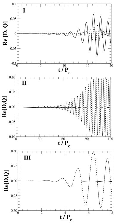
Figure 1: Diagnostics $D$ and $Q$ as a function of $t/P_{\rm c}$ for 3 differentially rotating stars (see Table 1). Solid and dotted lines denote the values of $D$ and $Q$, respectively. The Roman numeral in each panel corresponds to the model of the differentially rotating stars, respectively. Hereafter $P_{\rm c}$ represents the central rotation period.

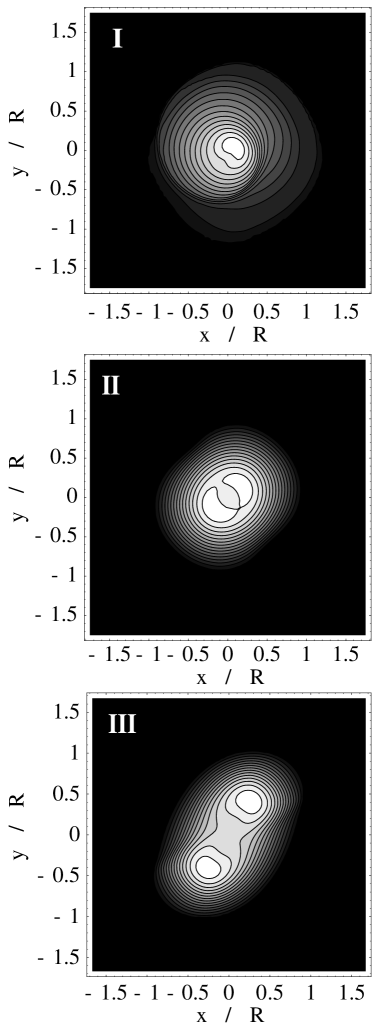
Figure 2: Density contours in the equatorial plane for 3 differentially rotating stars (see Table 1). Models I, II, and III are plotted at the parameter ($t/P_{\rm c}$, $\rho_{\rm max}/\rho_{\rm max}^{(0)}$) = ($16.3$, $3.63$), ($132$, $1.25$), and ($5.49$, $1.20$), where $\rho_{\rm max}$ is the maximum density, $\rho_{\rm max}^{(0)}$ is the maximum density at $t=0$, and $R$ is the equatorial radius at $t=0$. The contour lines denote densities $\rho/\rho_{\rm max}=10^{-(16-i)d}(i=1,\cdots,15)$ for model I and $\rho/\rho_{\rm max}=6.67(16-i)\times 10^{-2}(i=1,\cdots,15)$ for models II and III, respectively.

The time evolutions of dipole diagnostic and the quadrupole diagnostic are plotted in Fig. 1. We determine that the system is stable to $m=1$ ($m=2$) mode when the dipole (quadrupole) diagnostic remains small throughout the evolution, while the system is unstable when the diagnostic grows exponentially at the early stage of the evolution. It is clearly seen in Fig. 1 that the star is more unstable to the one-armed spiral mode for model I, and more unstable to the bar mode for models II and III. In fact, both diagnostics grow for model I. The dipole diagnostic, however, grows more markedly than the quadrupole diagnostic, indicating that the $m=1$ mode is the dominant unstable mode.

The density contour of the differentially rotating stars are shown in Fig. 2. It is clearly seen in Fig. 2 that one-armed spiral structure is formed at the intermediate stage of the evolution for model I, and that bar structure is formed for models II and III once the dynamical instability sets in.

We also show gravitational waves generated from dynamical one-armed spiral and bar instability in Fig. 3. For $m=1$ modes, the gravitational radiation is emitted not by the primary mode itself, but by the $m=2$ secondary harmonic which is simultaneously excited, albeit at a lower amplitude. Unlike the case for bar-unstable stars, the gravitational wave signal does not persist for many periods, but instead is damped fairly rapidly.

III Canonical Angular Momentum

We introduce canonical angular momentum following Ref. FS78 to diagnose oscillations in rotating fluids. For adiabatic linear perturbations on a perfect fluid configuration in stationary, axisymmetric spacetime, it is possible to introduce canonical conserved quantities. Since we only use canonical angular momentum $J_{\rm c}$ in this paper, we write down its explicit form as

$$J_{\rm c} = m\int(\Re[\sigma]-m\Omega)\rho|\xi|^{2}d^{3}x$$ (10)

$$-2m\int\rho\varpi\Omega\cdot\Im[\xi^{\varpi}\xi^{\varphi*}]d^{3}x,$$

where $\sigma$ is the eigenfrequency, $\xi^{i}$ is Lagrangian displacement vector. Note that total canonical angular momentum becomes zero when dynamical instability sets in.

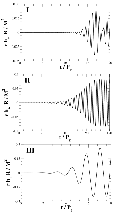
Figure 3: Gravitational waveform for 3 differentially rotating stars (see Table 1) as seen by a distant observer located on the rotational axis of the equilibrium star.

Next we apply the method of canonical angular momentum to the linearized oscillations of a cylinder. We prepare two $m=1$ stable modes (A-i, A-iii) and one $m=1$ unstable mode (A-ii), summarized in Table 2. We plot the integrand of canonical angular momentum $\varpi j_{\rm c}$

$$j_{c}=m(\Re[\sigma]-m\Omega)\rho|\xi|^{2}-2m\rho\varpi\Omega\cdot\Im[\xi^{\varpi}\xi^{\varphi*}],$$ (11)

for $m=1$ mode in Fig. 4. We define corotation radius $\varpi_{\rm crt}$ of modes as $\Re[\sigma]-m\Omega(\varpi)=0$. This means that the pattern speed of mode coincides with the local rotational frequency of background flow there. We find that the distribution of canonical angular momentum changes its sign around corotation radius in $m=1$ unstable case, and that it is positive for $\varpi<\varpi_{\rm{crt}}$, while it is negative for $\varpi>\varpi_{\rm{crt}}$. The behavior of the canonical angular momentum suggests us that this instability is related to the existence of corotation point inside the cylinder. We also find that the positive case of the canonical angular momentum (A-iii) corresponds to the case when the pattern speed of the mode is faster than the rotation of cylinder in all radius, while the negative (A-i) corresponds to the opposite. We also check the low $T/|W|$ bar instability in cylindrical model and find that the same behavior as $m=1$ mode (B) appears in the distribution of the canonical angular momentum density (Fig. 5).

Table 2: Parameters for equilibrium gaseous fluid and eigenfrequency

Model	$\Omega_{\rm c}/\Omega_{\rm s}$	$T/|W|$	$\sigma/\Omega_{\rm c}$	$\varpi_{\rm{crt}}/\varpi_{\rm s}$
A-i	11.34	0.460	$-0.245$	—
A-ii	11.34	0.460	$0.551+0.0315i$	0.281
A-iii	11.34	0.460	$1.15$	—
B	13.00	0.170	$0.327+0.0126i$	0.507

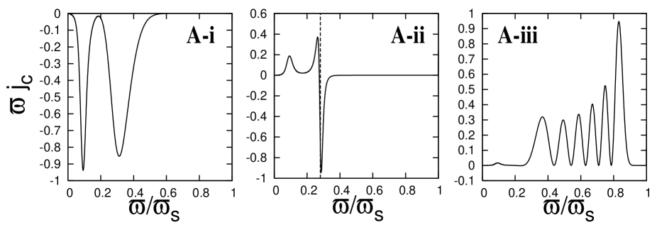
Figure 4: Distribution of canonical angular momentum density for $m=1$ unstable mode (see Table 2). Vertical dashed line represents the location of corotation radius of the mode. The Roman character in each panel corresponds to the model of the cylindrical gaseous fluid, respectively. Note that we normalized the distribution of the canonical angular momentum in an appropriate value, since the eigenfunction can be scaled arbitrarily.

Figure 5: Distribution of canonical angular momentum density for $m=2$ unstable mode (see Table 2). The Roman character in the panel corresponds to the model of the cylindrical gaseous fluid. Vertical dashed lines mark the locations of corotation radius of the mode.

We furthermore investigate $m=2$ instability of Bardeen disk and classical bar instability of Maclaurin spheroid. In these cases, the canonical angular momentum density that is analytically obtained is zero in all cylindrical radius. Therefore the behavior of the canonical angular momentum density shows a clear contrast between $m=1$, $2$ instability with high degree of differential rotation and $m=2$ classical instability of uniformly rotating fluid.

Finally, we adopt the method of canonical angular momentum to the nonlinear hydrodynamics. We identify the complex eigenfrequency and the corotation radius from dipole or quadrupole diagnostics which is summarized in Table 3. Note that we read off the eigenfrequency from those plots at the early stage of the evolution. The Eulerian perturbed velocity is defined by subtracting the velocity at equilibrium from the velocity. The Lagrangian displacement vector is extracted by using a linear formula for a dominant mode in each case.

Table 3: Eigenfrequency and the corotation radius of 3 differentially rotating stars

Model	$\sigma$ $[\Omega_{\rm c}]$	$\varpi_{\rm crt}$ $[R_{\rm eq}]$
I	$0.590+0.0896i$	$0.167$
II	$0.284+0.0121i$	$0.492$
III	$0.757+0.200i$	—

We show the snapshots of canonical angular momentum density in Fig. 6. Since we determine the corotation radius using the extracted eigenfrequency and the angular velocity profile at equilibrium, the radius does not change throughout the evolution. For low $T/|W|$ dynamical instability, the distribution of the canonical angular momentum drastically changes its sign around the corotation radius, and the maximum amount of canonical angular momentum density increases at the early stage of evolution. This means that the angular momentum flows inside the corotation radius in the evolution. On the other hand, for high $T/|W|$ dynamical instability that is related to the classical bar instability, the distribution of the canonical angular momentum is smooth with no particular feature and tends to have a positive portion outside. This means that the canonical angular momentum flows outwards in the evolution, which is in clear contrast to the case of low $T/|W|$ one.

From these different behaviors of the distribution of the canonical angular momentum, we see that the mechanisms working in the low $T/|W|$ instabilities and the classical bar instability may be quite different, i.e., in the former the corotation resonance of modes are essential, while the instability is global in the latter case.

IV Discussion

We have studied the nature of dynamical one-armed spiral instability in differentially rotating stars both in linear eigenmode analysis and in hydrodynamic simulation using canonical angular momentum distribution.

We have found that the one-armed spiral instability occurs around the corotation radius of the star by investigating the distribution of the canonical angular momentum. We have also found by investigating the canonical angular momentum that the instability grows through the inflow of the angular momentum inside the corotation radius. The feature also holds for the dynamical bar instability in low $T/|W|$, which is in clear contrast to that of classical dynamical bar instability in high $T/|W|$. Therefore the existence of corotation point inside the star plays a significant role of exciting one-armed spiral mode and bar mode dynamically in low $T/|W|$.

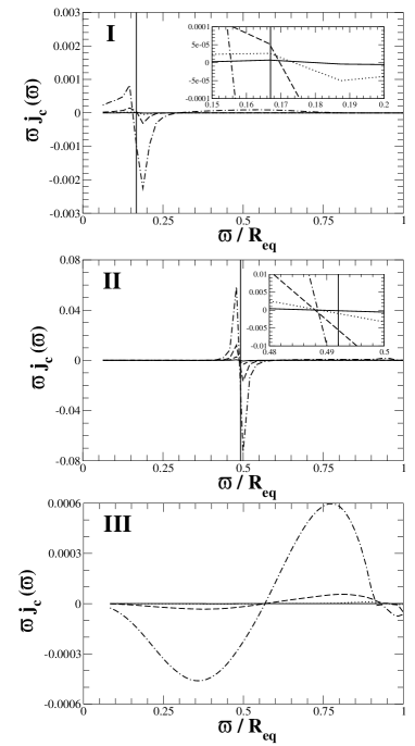
Figure 6: Snapshots of the canonical angular momentum distribution $\varpi j_{\rm c}(\varpi)$ in the equatorial plane for 3 differentially rotating stars (see Table 1). Solid, dotted, dashed, and dash-dotted line represents the time $t/P_{\rm c}=$(3.47, 6.93, 10.40, 13.86) for model I, $t/P_{\rm c}=$(45.68, 56.43, 67.18, 77.97) for model II, and $t/P_{\rm c}=$(1.10, 2.19, 3.29, 4.39) for model III, respectively. Note that vertical line in panels I and II denotes the corotation radius of the star (model III does not have a corotation radius). We also enlarged the figure around the corotation radius for panels I and II, which is presented in the right upper part of each panel. Although our method of determining the corotation radius is not precise, we clearly find that the distribution significantly changes around the corotation radius.

Finally, we mention the feature of gravitational waves generated from this instability. Quasi-periodic gravitational waves emitted by stars with $m=1$ instabilities have smaller amplitudes than those emitted by stars unstable to the $m=2$ bar mode. For $m=1$ modes, the gravitational radiation is emitted not by the primary mode itself, but by the $m=2$ secondary harmonic which is simultaneously excited, possibly through non-linear self-coupling of m=1 mode. (Remarkably the precedent studies CNLB01 ; SBS03 found that the pattern speed of $m=2$ mode is almost the same as that of $m=1$ mode, which suggest the former is the harmonic of the latter.) Unlike the case for bar-unstable stars, the gravitational wave signal does not persist for many periods, but instead is damped fairly rapidly.

References

- (1) S. Chandrasekhar, Ellipsoidal Figures of Equilibrium, (Yale Univ. Press, New York, 1969), 61.
- (2) J. Tassoul, Theory of Rotating Stars (Princeton Univ. Press, Princeton, 1978).
- (3) M. Shibata, S. Karino, and Y. Eriguchi, Mon. Not. R. Astron. Soc. 334, L27 (2002); 343, 629 (2003).
- (4) J. E. Tohline, and I. Hachisu, Astrophys. J. 361, 394 (1990).
- (5) J. M. Centrella, K. C. B. New, L. L. Lowe, and J. D. Brown, Astrophys. J. 550, L193 (2001).
- (6) M. Saijo, T. W. Baumgarte, and Shapiro, Astrophys. J. 595, 352 (2003).
- (7) J. C. B. Papaloizou, J. E. Pringle, Mon. Not. R. Astron. Soc. 208, 721 (1984).
- (8) A. Watts, N. Andersson, D. I. Jones, Astrophys. J. 618, L37 (2005).
- (9) J. Ostriker, Astrophys. J. Suppl. 11, 167 (1965).
- (10) M. Saijo and S’i. Yoshida, in preparation (2005).
- (11) J. L. Friedman and B. F. Schutz, Astrophys. J. 221, 937 (1978).