Projection effects in cluster mass estimates : the case of MS2137-23

We revisit the mass properties of the lensing cluster of galaxies MS2137-23 and assess the mutual agreement between cluster mass estimates based on strong/weak lensing, X-rays and stellar dynamics. We perform a thorough elliptical lens modelling using arcs and their counter-images in the range $20\lesssim R\lesssim 100$ kpc and weak lensing ($100\lesssim R\lesssim 1000$ kpc). We confirm that the dark matter distribution is well consistent with an NFW profile with high concentration $c\sim 11.7\pm 0.6$.
We further analyse the stellar kinematics data of Sand et al. (2004) with a detailed modelling of the line-of-sight velocity distribution of stars in the cD galaxy and quantify the small bias due to non-Gaussianity of the LOSVD. After correction, the NFW lens model is unable to properly fit kinematical data and is a factor of $\sim 2$ more massive than suggested by X-rays analysis (Allen et al. 2001).
The discrepancy between projected (lensing) and tridimensional (X-rays,dynamics) mass estimates is studied by assuming prolate (triaxial) halos with the major axis oriented toward the line-of-sight. This model well explains the high concentration and the misalignement between stellar and dark matter components $(\Delta\psi\sim 13^{\circ})$.
We then calculate the systematic and statistical uncertainties in the relative normalization between the cylindric $M_{2}(<r)$ and spherical $M_{3}(<r)$ mass estimates for triaxial halos. These uncertainties prevent any attempt to couple 2D and 3D constraints without undertaking a complete tridimensional analysis. Such asphericity/projection effects should be a major concern for comparisons between lensing and X-rays/dynamics mass estimates.

1 Introduction

The issue of the late non-linear evolution of cosmic structure is essentially addressed via large N-body cosmological simulations. It is important to test their validity by comparing the small scale matter distribution to numerical predictions. Two observations act as key-tests for the CDM paradigm: the mass distribution of dark matter halos (radial density profile and triaxiality) and the abundance of sub-halos within main halos. This work focuses on the former issue.

Most CDM simulations predict a universal profile of the general form:

$$\rho(r/r_{s})=\rho_{s}(r/r_{s})^{-\alpha}\left(1+r/r_{s}\right)^{\alpha-3}\,,$$ (1)

with an inner slope $\alpha$ ranging between $\alpha=1$ and $\alpha=1.5$ (Navarro et al. 1997; Moore et al. 1998; Ghigna et al. 2000; Jing & Suto 2000). The parameters $r_{s}$ and $\rho_{s}$ can be related to the halo mass (Bullock et al. 2001; Eke et al. 2001). Though more recent simulations propose a slightly different universal analytical form (Stoehr et al. 2002; Navarro et al. 2004).

The global agreement between observations and simulations is subject to controversy. The inner slope of dark matter halos of low surface brightness (LSB) dwarf galaxies as inferred from rotation curves tends to favor soft cores with $\alpha\lesssim 0.2$ (e.g.  Salucci 2001; de Blok et al. 2003; Gentile et al. 2004), leading to the so-called cusp-core debate. Many observations have focused on LSB galaxies because their baryonic content can be neglected and the dark matter distribution in the halo shall match simulations. However, departs from axisymmetry (triaxial halos) make the interpretation of rotation curves more complex and could reconcile observations and CDM predictions (Hayashi et al. 2004). The question of the very central mass profile on dwarfs scales is still open…

Recently a similar discrepancy at clusters of galaxies scales is claimed by Sand et al. (2002, 2004, hereafter Sa04). Using HST images (allowing the modelling of strong gravitational lensing configurations) together with Keck spectroscopy (providing the radial velocity dispersion of stars in the central cD galaxy of the cluster, the BCG) on a sample of six clusters, these authors found that the inner slope of the dark matter halo must be significantly flatter than that measured in simulations. Typically, on a subsample of three clusters with radial arcs, they found an inner slope $\alpha=0.52\pm 0.05$ (68%CL). This result takes advantage of the joint constraints provided by lensing and stellar kinematics. However, the lensing part of the analysis of Sa04 has been independently discussed by Bartelmann & Meneghetti (2004) and Dalal & Keeton (2003) because they did not take into account the lens ellipticity when using the critical lines radii as a constraint on the density profile. These two latter authors found that the mass profile is consistent with a NFW model. The analysis of Sa04 couples 2D projected (from lensing that deal with mass enclosed in the cylinder of radius $R$) and 3D tridimensional (from stellar dynamics which project an indirect information on the mass enclosed in the sphere of radius $r$) mass estimates.

Comparing lensing and X-rays cluster mass estimates is another way to couple 2D and 3D mass constraints. The overall agreement between X mass and the mass enclosed in the Einstein radius of clusters are been addressed by various authors (Miralda-Escude & Babul 1995; Allen 1998; Wu 2000; Arabadjis et al. 2004; Smith et al. 2005). In most cases, slightly depending on the presence of cooling flows or the degree of relaxation of the cluster, strong lensing mass estimates are often larger by a factor $\gtrsim 1.5$.With better S/N data, there is an increasing evidence that the assumption of spherical symmetry starts being oversimplistic and may play a important role in this systematic trend (Piffaretti et al. 2003; De Filippis et al. 2005; Oguri et al. 2005; Hennawi et al. 2005).

In this paper, we focus on the density profile of the cluster MS2137-21 which is part of the Sa04 sample and search for further evidence for triaxiality in this peculiar cluster. In Sect. 2 we present the strong and weak lensing modelling of MS2137 with a NFW model and show that it is consistent with all the lensing data at hand from 10 kiloparsecs to 1 megaparsec. In Sect. 3 we develop a detailed method for the analysis of stellar kinematics and apply it to the best fit NFW model derived in the previous section. We then discuss the overall agreement between lensing mass estimates and the constraints from the stellar kinematics and X-rays observations of Allen et al. (2001). In Sect. 4 we investigate the origin on the systematic overerestimate of lensing mass estimates as compared to that of 3D analyses, and show that the tridimensional shape of halos (prolate, triaxial) is likely to explain such discrepancies. In Sect. 5 we calculate the statistical properties of the relative normalization between 2D and 3D mass estimates of triaxial halos. We discuss our results and conclude in Sect. 6.

Throughout this paper, we assume a $\Omega_{m}=0.3$, $\Omega_{\Lambda}=0.7$ and $H_{0}=70\,h_{\rm 70}\,{\rm km\,s}^{-1}\,{\rm Mpc}$, leading to the scaling $1\arcsec=4.59\,h_{\rm 70}^{-1}\,{\rm kpc}$.

2 Lens modelling

2.1 Optical data and $\chi^{2}$ definition

In this section we focus on the density profile modeling using lensing constraints only. The lens properties of the cluster of galaxies have been extensively studied (Fort et al. 1992; Mellier et al. 1993; Miralda-Escudé 1995; Bartelmann 1996; Hammer et al. 1997; Gavazzi et al. 2003; Sand et al. 2002, 2004; Dalal & Keeton 2003). The cluster’s redshift is $z_{l}=0.313$ and both radial and tangential arcs lie at $z_{s}=1.501$ (Sand et al. 2002), leading to the critical surface density $\Sigma_{\rm crit}=2.39\times 10^{9}\,h_{70}\,{\rm M}_{\odot}\,{\rm kpc}^{-2}$.

Our analysis builds on the previous work of Gavazzi et al. (2003) (Hereafter G03). More precisely, we use 26 multiple conjugate knots in the tangential and radial arcs systems. The method and the knots location are presented in G03. Here, we inflate the uncertainties on knot positions in order to account for possible bad associations. Basically, the mean positional error is raised to the more realistic value $\sigma_{x}=0\aas@@fstack{\prime\prime}3$. After a more detailed analysis of images, the G03 value $=0.18\arcsec$ turns out to be underestimated. Moreover there was a mistake in the calculation of error bars for model parameters in this earlier paper. The uncertainty on each knot location is just increased by the same amount, so we do not expect any change in the best fit model. Dalal & Keeton (2003) proceeded in the same way by inflating the G03 errors up to a value of $1\arcsec$ which is far too much. We stress that the error bars of G03 on the best fit parameters are larger than the ones we shall present in the following although they assumed smaller uncertainties on knots locations. This is a clear evidence for an error in the analysis. The present updated results should be considered as correct. We also exclude constraints from the fifth central demagnified image reported in G03 since its detection is marginal and is not confirmed by Sa04. We use a personal ray-tracing inversion code which includes many aspects of the lensmodel software (Keeton 2001a, b). In particular, we adopt the same source plane $\chi_{\rm src}^{2}$ definition.

In addition, we simultaneously include weak lensing constraints also presented in G03. The catalogue of background “weakly lensed” galaxies comes from VLT/FORS and VLT/ISAAC images for which we were able to derive a good estimate of photometric redshifts using $UBVRIJK$ bands. We fully compute the likelihood as a function of model parameters (Schneider et al. 2000; King & Schneider 2001).

$$\mathcal{L}_{\rm wl}=\prod_{i=1}^{N_{\rm bg}}p(e_{i})$$ (2)

where $e_{i}$ is the observed ellipticity of the background galaxy. We have

$$p(e_{i})=p_{s}(e_{s}(e_{i},g_{i}))\left|\frac{{\rm d}e_{s}}{{\rm d}e_{i}}\right|,$$ (3)

$e_{s}$ being the source ellipticity and $g_{i}=g(\@vec{\theta}_{i},z_{i})$ is the reduced shear. See Geiger & Schneider (1998) for the description of the relation $e_{s}(e_{i},g)$ and for the corresponding transformation Jacobian. Ellipticities are measured on the I band image. We improved the previous analysis of G03 and built a new PSF smearing correction pipeline based on the KSB method (Kaiser et al. 1995) but leading to a better weighting scheme (Gavazzi et al. 2004). We fully take into account redshift information, either photometric for weak lensing or spectroscopic for strongly lensed arcs. The use of photometric redshifts to select the sample of background galaxies avoids the problem of contamination by foreground unlensed galaxies (Broadhurst et al. 2005). The global $\chi^{2}$ for lensing is :

$$\chi^{2}_{\mathrm{lens}}=\chi^{2}_{\mathrm{src}}-2\ln\mathcal{L}_{\rm wl}\;.$$ (4)

We use the minuit library to minimize this $\chi^{2}$. The error analysis is performed using both minuit facilities and Monte-Carlo Markov Chains (MCMC) based on the implementation of Tereno et al. (2005). We chose to use MCMCs because minuit has difficulties to draw $\Delta\chi^{2}$ contours in the parameter space when there are strong degeneracies. In order to fasten the convergence of the chains, we previously run many minuit optimizations starting from a broad range of initial conditions. From the well defined best fit minimum position, we started up to five chains with each of them ending with $6\times 10^{4}$ relevant iterations. The convergence assessment was done in the same way as in Tereno et al. (2005).

2.2 Luminosity profile

We fitted the central cD surface brightness on the F702/WFPC2 Hubble Space Telescope image (Hammer et al. 1997) with a general projected stellar density profile assuming that all stars have a constant mass-to-light ratio. We assumed the following analytic expression for the three-dimensional radial distribution of stars :

$$\rho_{*}(r)=\rho_{s*}x^{-\delta}(1+x)^{\delta-4},$$ (5)

where $x=r/r_{s*}$, $r_{s*}$ is a scale radius. We considered the particular values $\delta=1$ for the Hernquist profile Hernquist (1990) and $\delta=2$ for the Jaffe profile Jaffe (1983) which were added to the 2 dimensional galaxy model fitting software galfit (Peng et al. 2002). Before fitting the luminosity profile is convolved by the HST/F702 PSF. The Hernquist fit gives an axis ratio $q_{*}=b/a=0.83\pm 0.12$, a scale radius $r_{s*}=11.1\pm 1.9\,h_{\rm 70}^{-1}\,{\rm kpc}=2\aas@@fstack{\prime\prime}4\pm 0\aas@@fstack{\prime\prime}1$ and a reduced $\chi^{2}/{\rm dof}=10.2$. This latter value could be noticeably decreased by taking into account a rotation of the major axis position angle within the inner 3 arcsec (see Fig. 2 of G03). We also tried to fit a Jaffe profile as proposed by Sa04 but we found a much worse $\chi^{2}/{\rm dof}=99.0$. However, Sa04 found that the stellar density profile is well fitted by a De Vaucouleur model which is bracketed by the Hernquist and Jaffe models. Therefore we consider that the stellar component is well modeled by an Hernquist density profile with $r_{s*}=11.1\,h_{\rm 70}^{-1}\,{\rm kpc}$ and a total rest frame V band luminosity $L_{V}=4.77\pm 0.40\times 10^{11}\,\,h_{\rm 70}^{-2}\,L_{\odot}$ (Sa04). The mass content in stars is $M_{*}=2\pi\rho_{s*}r_{s*}^{3}q_{*}\equiv\Upsilon_{V}L_{V}$ where $\Upsilon_{V}$ is the rest-frame V band stellar mass-to-light ratio.

Throughout the paper, we shall discuss the consequences of this particular choice. At this level, we expect the effect of this choice to be more important for stellar kinematics than for lensing. This can be understood because strong lensing constraints probe the total density profile well beyond the stellar scale radius where Hernquist, Jaffe or De Vaucouleur profiles are very similar (see Fig. 2 of Sa04).

Figure 1: NFW best fit model for strong lensing constraints.   Left: Caustic lines with the position of the 26 knots in the source plane.   Right: Critical lines with the observed (resp. model) position of the 26 knots represented with circles (resp. + signs). Geometrical units are arcsec.

2.3 NFW dark matter density profile

The lens is decomposed into two components. The cD stellar component is modeled by the elliptical Hernquist profile of the previous section. The stellar mass-to-light ratio $\Upsilon_{V}$ is treated as a free parameter with a broad uniform prior $1.5\leq\Upsilon_{V}\leq 10$ whereas the scale radius, orientation and ellipticity are fixed by the observed light distribution. The dark matter halo is modeled with an elliptical NFW density profile:

$$\rho_{\rm DM}(r)=\rho_{s}\,(r/r_{s})^{-1}\left(1+r/r_{s}\right)^{-2}\,.$$ (6)

The lens properties of such a density profile are presented in (Bartelmann 1996). We used numerical integrations algorithms for the elliptical Hernquist and NFW density profiles (Keeton 2001a). The model has five free parameters :

• the dark halo scale radius : $r_{s}$,

• the characteristic convergence : $\kappa_{s}\equiv\rho_{s}r_{s}/\Sigma_{\rm crit}$,

• the dark halo axis ratio : $q=b/a$,

• the dark halo major axis position angle : $\psi_{0}$,

• the stellar mass-to-light ratio : $\Upsilon_{V}\equiv M_{*}/L_{V}$.

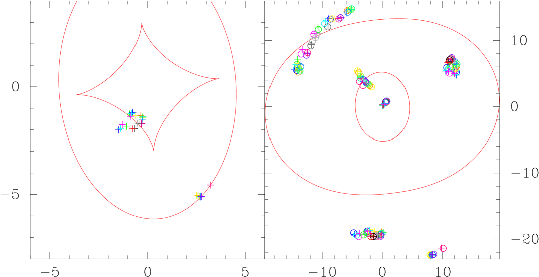
Fig. 1 shows the best fit NFW strong lensing configuration. One can see the source and image planes with caustic and critical lines together with the location of the 26 multiply images knots. Every observed point (circle) is well reproduced by the model (+ signs). The source associated to the tangential arc is clearly crossing the corresponding caustic line (inner astroid) whereas one can only see the part of the source associated to the radial arc that is inside the radial caustic (since the part outside the caustic is not multiply imaged and is useless for modelling). The central image associated to the tangential system is plotted but is not taken into account in the modelling. Besides the critical lines location (the only constraint used by Sa04), our model also remarquably explains the position of counter-images, the azimuthal configuration, the length and width of arcs.

	(SL)	(SL+WL)	(1)	unit
$\kappa_{s}$	$0.67\pm 0.05$	$0.66\pm 0.03$	$0.30\pm 0.15$
$r_{s}$	$158^{+15}_{-13}$	$162^{+11}_{-9}$	$160\pm 30$	$\,h_{\rm 70}^{-1}\,{\rm kpc}$
$r_{\rm 200}$	$1.88\pm{0.05}$	$1.89\pm{0.04}$	$1.39^{+0.49}_{-0.38}$	$\,h_{\rm 70}^{-1}\,{\rm Mpc}$
$M_{\rm 200}$	$7.56^{+0.63}_{-0.54}$	$7.72^{+0.47}_{-0.42}$	-	$10^{14}\,h_{\rm 70}^{-1}M_{\odot}$
$c$	$11.92^{+0.77}_{-0.74}$	$11.73\pm 0.55$	$8.7^{+1.2}_{-0.9}$
$q$	$0.774\pm 0.010$	$0.777\pm 0.007$	-
$\psi_{0}$	$5.86\pm 0.14$	$5.88\pm 0.13$	-	deg
$\Upsilon_{V}$	$2.40\pm 0.45$	$2.48\pm 0.39$	-	$\,h_{\rm 70}\,(M/L)_{\odot}$

Table 1: Best fit NFW model parameters and their 68% CL uncertainty (marginalized over all the other parameters). (SL) corresponds to a model in which weak lensing constraints are ignored whereas (SL+WL) takes both strong and weak lensing constraints into account. (1) refers to the CHANDRA X-rays values of Allen et al. (2001). The apparent disagreement between their estimates and ours is discussed in the text.

The model requires a rest frame V band stellar mass-to-light ratio $\Upsilon_{V}=2.5\pm 0.4$. This value is in good agreement with expectations of evolution of $2\lesssim t\lesssim 4$ Gyr old stellar populations. The reason why the stellar mass content is so tightly constrained is that the stellar and dark matter components are not aligned. There is a position angle misalignment of $\Delta\psi=13^{\circ}$. This was first pointed out by G03. Otherwise, there would be a degeneracy between the relative contribution of dark matter and stars. Here the degeneracy is broken though the contribution of stars is subdominant at all scales (and a factor $\sim 2$ at the centre) as shown in Fig. 3. This situation well explains the small inaccuracy in the radial arc modelling highlighted in Sect. 4.2 of G03. By adding a small misaligned contribution under the form of stars at the center, one is able to twist to isopotentials and precisely reproduce the radial arc and its counter-image. See Romanowsky & Kochanek (1998) and Buote et al. (2002) for a similar example. We shall turn back to this issue in Sect. 4.4 and appendix B. It is worth mentioning that changing the stellar mass profile to a Jaffe model does not make differences. The total (misaligned) stellar mass is well fixed by lensing.

Figure 2: Scatter plot showing the projection of MCMCs on some planes of the parameters space of the NFW lens modelling. The color codes for the ellipticity parameter according to the scale at the bottom right corner. The axes are the virial mass $M_{\rm 200}$, the concentration $c$ and the rest-frame V band stellar mass-to-light ratio $\Upsilon_{V}\equiv M_{*}/L_{V}$.

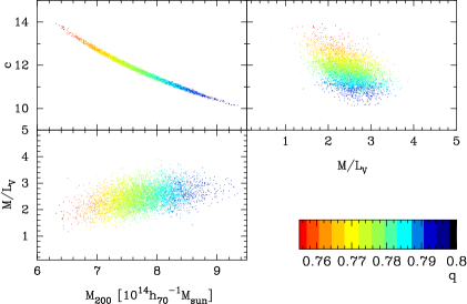
In Table 1 we present the best fit NFW model parameters in terms of more physical quantities like the virial radius $r_{\rm 200}$, the concentration parameter $c=r_{\rm 200}/r_{s}$ or the virial mass $M_{\rm 200}$ that all derive from $\kappa_{s}$, $r_{s}$ and $q$. At the best fit parameter set, the minimum $\chi^{2}$ value is $\chi^{2}/{\rm dof}=4931.20/4965=0.993$. When considering strong lensing constraints only, $\chi^{2}_{\rm src}/{\rm dof}=76.4/130=0.59$ showing that both strong and weak lensing observations are well modeled. The (SL) and (SL+WL) columns detail how the best fit model is changed whether weak lensing constraints are added to the model or not. Basically, errors are just reduced and no significant change in the best fit parameters value is observed. Fig. 2 shows the degeneracies between the concentration parameter, virial mass, stellar mass-to-light ratio and ellipticity (color-coded).

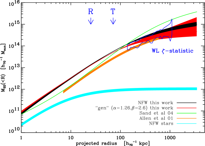
Fig. 3 shows the radial projected mass profile for the best fit NFW+stellar components as well as a detail of the stellar component. The thickness of curves is representative of the 1$-\sigma$ uncertainties. This is done by considering many points of the MCMCs that stand within the 1-$\sigma$ contour about the best fit model.

Figure 3: Projected total mass (stars+DM) profile within cylinder of radius $R$ for the best fit NFW model (black), the best fit general “gen” model with $\alpha=1.26$ and $\beta=2.6$ (red), the best fit model of Sand et al. (2002, 2004) (green) and the best fit NFW model from X-rays constraints (Allen et al. 2001) (orange). The contribution of stars for the NFW model is the cyan dashed curve. The width on the curves is representative of the 1$-\sigma$ uncertainties (except for the Sa04 profile). The blue region is the domain constrained by the weak-lensing $\zeta$-statistic. The location of the tangential (resp. radial) critical lines is reported by a blue “T” (resp. “R”). The “gen” and NFW models match well from the center to the inner radius probed by weak-lensing. Beyond, their are consistent within the weak-lensing uncertainties. For $R\lesssim 40\,{\rm kpc}$ both profiles present large (a factor $\sim 2$) discrepancies with the curves inferred by Sa04 and Al01. See text.

2.4 A more general profile for dark matter

The quality of the fit is such that very few departs from the NFW model we found are allowed. In order to check how restrictive the analytical form (6) is, we also assumed the following profile for the dark matter component (Wyithe et al. 2001)

$$\rho_{\rm DM}(r)=\rho_{s}\,x^{-\alpha}\left(1+x^{2}\right)^{(\alpha-\beta)/2}\>,$$ (7)

with $x=r/r_{s}$ the radius in units of a scale radius $r_{s}$ and two more free parameters: the asymptotic inner and outer slopes $\alpha$ and $\beta$ respectively. We will refer to this model as the “gen” profile. This model slightly differs from the generally assumed generalised gNFW model $\rho\propto x^{-\alpha}\left(1+x\right)^{\alpha-3}$ and a comparison to previous studies is not straightforward. Nevertheless we chose this model because it is computationally tractable even with elliptical symmetry (Chae et al. 1998; Chae 2002) and allows another degree of freedom since the outer slope is not fixed.

For the best fit model, we have $\chi^{2}/{\rm dof}=4915.90/4963=0.990$, and $\chi^{2}_{\rm src}/{\rm dof}=64.2/128=0.50$. Here again, the $\chi^{2}$ value is satisfying. We found $\Upsilon_{V}=2.09\pm 0.16$ also consistent with stellar evolution models, $\beta=2.69^{+0.32}_{-0.22}$ and $\alpha=1.262^{+0.013}_{-0.017}$.The constraints on $\alpha$ are very tight and show that lensing is inconsistent with any soft core $\alpha\ll 1$. However, it does not contradict the NFW behavior $\rho\propto r^{-1}$ at small scales because the fast transition $1+x^{2}$ in the “gen” profile differs from the NFW case $(1+x)$. This can clearly be seen in Fig. 3 where the projected NFW and “gen” mass profiles match over a broad radius range ($r\lesssim 100\,{\rm kpc}$). The differences at larger scales are still within the weak lensing uncertainties. Consequently, we can faithfully trust the radial behavior of the lensing deduced mass profile of the NFW model between $10<R<1000\,{\rm kpc}$.

Here again, changing the Hernquist stellar profile to a Jaffe model does not change our results.

2.5 Comments

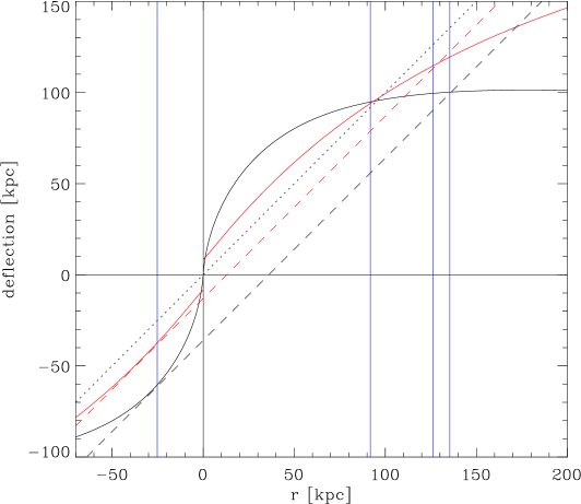
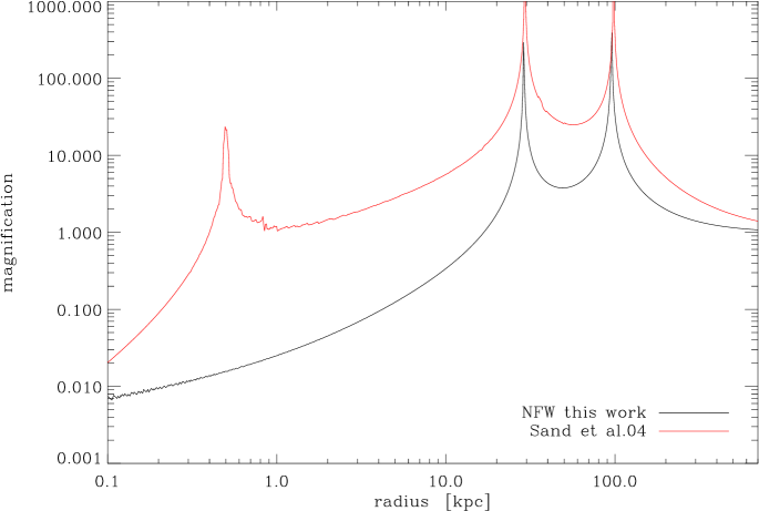
Fig. 3 also shows the best fit model of Sa04 which presents strong discrepancies with both our NFW and “gen” models. Though the projected mass at the tangential arc radius ($\sim 100\,{\rm kpc}$) matches our estimates, the model of Sa04 is inconsistent with most lensing constraints. They imposed the radial critical line to fit the observations but their model cannot reproduce the radial arc length and its counter-images well, nor the tangential arc width and weak lensing at $R\gtrsim 200\,{\rm kpc}$. This can be understood by comparing the circularly averaged deflection $\@vec{\alpha}$ profile of these models in the upper panel of Fig. 4. This plot is used to solve the lens equation graphically. The tangential critical radii (intersection of curves $\alpha(r)$ and $y=r$) are consistent from one model to another. As well the curves $\alpha(r)$ are tangent to the line $y=r+u$ at the same radial critical radius. But the intersections of $\alpha(r)$ and this line at the opposite side, which give the location of the counter-image of the radial arc, significantly differ ($\sim$ 2 arcsec). Moreover, we can see that the Sa04 model predicts a much more elongated radial arc that could extend very close to the lens center. This is clearly excluded by the data. It is worth noticing that the Sa04 model predicts another radial critical line at the very center ($r\sim 0.1\arcsec$) and globally higher magnifications since $\alpha(r)$ is close to the bisectrix $y=r$. The only models consistent with all lensing constraints are the ones similar to the NFW and the “gen” models.

The column (1) of Table 1 also resumes the NFW model parameters deduced from Chandra X-rays observations of Allen et al. (2001, hereafter Al01). The projected mass profile of their model is the orange thick curve on Fig. 3. This NFW profile is twice as low as our NFW and “gen” models over a range $10<R\lesssim 200\,{\rm kpc}$ (i.e. the factor $1/2$ in the value of $\kappa_{s}$ in table 1). At larger scales $R\gtrsim 300\,{\rm kpc}$, the Al01 mass profile becomes consistent with weak lensing and our models. X-rays (Al01) and stellar dynamics (Sa04) mass estimates agree at small scales $R\lesssim 50\,{\rm kpc}$.

Figure 4: Upper panel: Circularly averaged deflection angle for our best NFW fit (solid black curve) compared to that of Sa04 (solid red curve). From left to right, the blue vertical lines represent the radial and tangential critical radii, the Sa04 and our prediction of the radial arc counter-image. The critical radii match from one model to another but the radial arc lenght significantly differs. The dotted $y=r$ line gives the solution of the tangentiel critical radius. The dashed lines $y=r+u$ (with $u$ the source location) give the solution of the radial critical radius where it is tangent to the curve $y=r$. Lower panel: Magnification profile. The Sa04 model predicts high magnifications close to the center with another radial critical line at the very center ($r\sim 0.1\arcsec$).

3 Dynamics of stars in the BCG

The kinematical properties of stars in the central cD galaxy are studied in this section. Instead of using the standard Jeans equation to relate the gravitational potential and the velocity dispersion of tracers, we fully calculate the line-of-sight velocity distribution LOSVD via a thorough dynamical analysis which is detailed in appendix A. By doing so, we can estimate the biased velocity dispersion profile $\sigma_{\rm h_{4}}(R)$ in place of the true velocity dispersion of stars $\sigma_{\rm los}(R)$ due to the assumed gaussianity of absorptions lines.

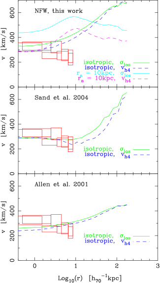
The analysis presented in appendix A shows that departs from gaussianity are kept at a low level for the lensing-deduced NFW mass model. For isotropic orbits Gaussianity is a fair assumption: $(\sigma_{\rm h_{4}}-\sigma_{\rm los})/\sigma_{\rm los}\sim-13\%$ at $R\sim 1\,{\rm kpc}$ and then decreases whereas departs can reach $\sim 30\%$ for anisotropic orbits. With this mass model we plot $\sigma_{\rm los}(R)$ and $\sigma_{\rm h_{4}}(R)$ on the top panel of Fig. 5 for different values of the anisotropy radius $r_{a}=\infty$ and $r_{a}=10\,h_{\rm 70}^{-1}\,{\rm kpc}$. The agreement between the measurements of Sa04 and $\sigma_{\rm h_{4}}(R)$ is better than with $\sigma_{\rm los}(R)$ but introducing anisotropy cannot improve the fit quality for $R\simeq 10\,{\rm kpc}$: the $\sigma_{\rm h_{4}}$ curve of the NFW model raises too fast whereas data indicate a declining tendency. However, if kinematical data would extend to slighly larger scales, we expect the profile to start raising and get closer to the model beyond a few tens of kpc as observed in others cD galaxies (Dressler 1979; Kelson et al. 2002).

We attempted to couple lensing and kinematical constraints by minimizing the merit function $\chi^{2}_{\mathrm{tot}}=\chi^{2}_{\mathrm{lens}}+\chi^{2}_{\mathrm{kin}}$, with

$$\chi^{2}_{\rm kin}=\sum_{i}^{N_{\rm bins}}\frac{({\sigma_{\rm h_{4}}}_{,i}-v_{\rm mes,i})^{2}}{\sigma_{\rm mes,i}^{2}}\>,$$ (8)

that accounts for kinematical constraints and $\chi^{2}_{\mathrm{lens}}$ defined in Eq. (4). $v_{\rm mes,i}$ and $\sigma_{\rm mes,i}$ are the measurements and errors of Sa04, and $N_{\rm bins}=8$. The inferred NFW model is marginaly changed as compared to the one found using lensing only. The NFW model is overconstrained by lensing and cannot fit the Sa04 kinematical data better. We find $\chi^{2}_{\rm kin}/N_{\rm bins}\sim 7$ for the best model. After $\chi^{2}$ minimization, the NFW model is still unable to reproduce the velocity decline at $R\gtrsim 4\,{\rm kpc}$.

Figure 5: Velocity dispersion $\sigma_{\rm los}(R)$ (solid green line) and biased velocity $\sigma_{\rm h_{4}}(R)$ (dashed blue line) profiles for isotropic orbits. The measurements of Sa04 are represented by red boxes.   Top: Our best fit NFW model. In this panel we have also represented another couple of ($\sigma_{\rm los}$,$\sigma_{\rm h_{4}}$) curves (cyan and magenta respectively) which correspond to an anisotropic Osipkov-Merritt case with $r_{a}=10\,{\rm kpc}$. The introduction of anisotropy does not improve the fit quality but leads to huge departs between $\sigma_{\rm los}$ and $\sigma_{\rm h_{4}}$.   Middle: Best fit model of Sa04 which matches the data well.   Bottom: Best fit model of Al01, inferred from X-rays analysis. This model also matches the measurements of Sa01 whereas none of these latter profiles are consistent with lensing observations.

Changing the Hernquist stellar light profile by a Jaffe model as proposed by Sa04 slightly improves the fit of kinematical data without altering the lens modelling (see Sect. 2.3). In this case, we have $\chi^{2}_{\rm kin}/N_{\rm bins}\sim 6.5$. The velocity dispersion curve raises a bit slower as compared to the Hernquist case. However, since the mass budget is dominated by dark matter, there is not much improvement. Lensing constraints are so tight that the allow region in the parameter space is completely fixed.

Likewise the “gen” model also fails in reproducing kinematical data although it has more free parameters. In this case, the inner slope $\alpha=1.250\pm 0.011$ is still fixed by lensing. The inferred stellar mass-to-light ratio is $\Upsilon_{V}=1.83\pm 0.14$ which is a rather low value. For the “gen” profile too, switching the stellar mass profile to a Jaffe model does not significantly improve the fit on kinematical data.

We have shown that departs from gaussian absorption lines induce a small bias which starts being important for dynamical systems with radial orbits. However this bias is unable to explain the discrepancy between lensing and kinematical mass estimates. Furthermore, such a bias cannot be advocated to explain the discrepancy between lensing and X-rays mass estimates. We can see on the central and bottom panels of Fig. 5 that the mass model of Sa04 fairly reproduces kinematical data, as well as the Al01 model (provided one addes the contribution of a central cD galaxy with $\Upsilon_{V}\sim 2.5$).

4 Discrepancies between mass estimates

At this level, let us resume the main problems that arise from the previous sections. A detailed lens modelling predicts a robust projected mass distribution that is consistent with NFW universal profiles. We have used a more general density profile for the dark matter halo in order to check that any other realistic mass profile should match our best fit NFW model over a broad range $20\lesssim R\lesssim 1000\,{\rm kpc}$. This family of models turns out to be inconsistent with the X-rays and kinematical mass estimates that are basically indirect measurements of the 3D mass within radius $r$. These two latter estimates are mutually consistent for $R\lesssim 50\,{\rm kpc}$.

Since lensing is sensitive to the integrated mass contrast along the line of sight, it is natural to expect overestimates due to fortuitous alignments with mass concentrations which are not physically related to the main halo of interest. Likewise, departs from spherical symmetry are observed in N-body simulations (e.g.  Jing & Suto 2002) and may bias lensing estimates. This question has been addressed by various authors (Bartelmann 1995; Cen 1997; Reblinsky & Bartelmann 1999; Clowe et al. 2004; Wambsganss et al. 2004; Hennawi et al. 2005). Conclusions about the importance of unrelated structures (large scale structure LSS) slightly differ from one author to another. Hoekstra (2003) found LSS to add noise to mass estimates on large scales but do not lead to biased estimates since on very large scales the skewness of the density field is negligible and light rays cross overdense regions as well as underdense ones. At smaller scales, this becomes obviously wrong and one expects fortuitous alignments of halos to modify the properties of halos. Wambsganss et al. (2004) claim that such effects can increase the lensing mass of $\sim 30-40\%$ of halos by a factor of $\sim 15-20\%$ whereas Hennawi et al. (2005) found this effect to change the lensing cross-sections of clusters by a smaller amount ($\lesssim 7\%$). See also (Hamana et al. 2004) and (Hennawi & Spergel 2005) for a discussion of projection effects on weak lensing cluster surveys.

On smaller scales, Metzler et al. (2001) found the mass of surrounding (sub)structures like filaments to add a significant contribution to the total convergence of a cluster-size lens whereas Clowe et al. (2004) showed that triaxiality is an important issue for lensing mass estimates. In the following, we shall focus on this paticular aspects which has been found to be important for lensing Oguri et al. (2003); Oguri & Keeton (2004) and/or X-rays observations (Piffaretti et al. 2003; De Filippis et al. 2005; Hennawi et al. 2005).

For a triaxial or oblate/prolate halo, the ratio of the mass enclosed in the cylinder of radius $R$ to the mass enclosed in the sphere of same radius will differ from that of a spherically symmetric situation. In order to illustrate projection effects, we consider an axisymmetric (either oblate or prolate) NFW density profile of the form :

$$\rho(m)=\frac{1}{m(1+m)^{2}}\quad\mathrm{,with}\;\;m^{2}=R^{2}+\frac{z^{2}}{q^{2}}\;.$$ (9)

The line of sight is along the $z$-axis and matches the major axis of a prolate halo when $q>1$ or the minor axis of an oblate halo when $q<1$. We can express $m\equiv r\lambda(q,\mu)$ with $\mu=\cos\theta$ and $\lambda^{2}=1+\mu^{2}(1/q^{2}-1)$. Numerical simulations predict triaxial halos with minor axis and intermediate axes $c$ and $b$ with a distribution given by (37). With these relations, we can numerically calculate the distribution of $q$ which is close to gaussian by approximating $q=c/\sqrt{b}=0.62\pm 0.12$ (resp. $q=1/\sqrt{bc}=1/0.64\pm 0.25$) for an oblate (resp. prolate) halo. This is a rough approximation since realistic triaxial halos are not systematically aligned with the line of sight but this gives an idea of acceptable values of the axis ratio $q$. .

Since we are interested in ratios between mass estimates we pay no attention to normalization constants and write the exact mass $M_{\rm true}(r;q)$ enclosed by the sphere of radius $r$ as

$$M_{\rm true}(r;q)=\int_{0}^{1}\frac{{\rm d}\mu}{\lambda^{3}}M_{\rm true}(\lambda r;1)\;,$$ (10)

where $M_{\rm true}(r;1)=\ln(1+r)-\frac{r}{1+r}$ for a NFW profile. We now calculate the mass $M_{\rm lens}(r;q)$ (resp. $M_{\rm kin}$, $M_{\rm X}$) as it would be found from lensing (resp. stellar kinematics, X-rays) measurements performed assuming spherical symmetry.

4.1 Projection effect on lensing

Since lensing measures the projected mass along the line of sight and owing to the fact that the major/minor axis is aligned, the net effect of asphericity is to multiply the surface mass density by $q$. So, we can write

$$M_{\rm lens}(r;q)=qM_{\rm true}(r;1)\;.$$ (11)

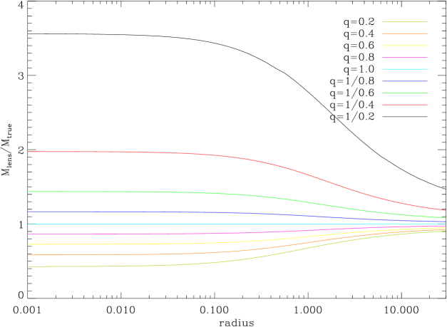
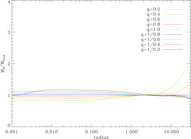
We plot the ratio $M_{\rm lens}(r;q)/M_{\rm true}(r;q)$ as a function of radius for various values of the axis ratio $q$ on the top panel of Fig. 6. We can observe strong discrepancies for extreme values of the axis ratio. Departs between lensing and true masses tend to vanish at large scale. Thus, one expects a lower effect of asphericity on weak lensing based mass estimates.

4.2 Projection effect on kinematics

Regarding stellar kinematics, projection effects are much more complex because stars are expected to move faster along the major axis and boost the mass estimate. Assuming a distribution function of stars of the form $f(E,L_{z})$ and a reduced gravitational potential $\Psi(R,z)$ the Euler–Jeans equations read :

$$\frac{1}{\nu}\partial_{R}(\nu\overline{v_{R}^{2}})+\frac{\overline{v_{R}^{2}}-\overline{v_{\phi}^{2}}}{R}=\partial_{R}\Psi$$ (12a)

$$\frac{1}{\nu}\partial_{z}(\nu\overline{v_{z}^{2}})=\partial_{z}\Psi\;.$$ (12b)

(Chandrasekhar 1960; Hunter 1977; Binney & Tremaine 1987). Thus, we can express the components of the velocity ellipsoid:

$$\nu\overline{v_{R}^{2}}=\nu\overline{v_{z}^{2}}= -\int_{z}^{\infty}{\rm d}z^{\prime}\,\nu\partial_{z}\Psi$$ (13a)

$$\nu R\Omega^{2}= -\int_{z}^{\infty}{\rm d}z^{\prime}\,\left[\partial_{R}\nu\partial_{z}\Psi-\partial_{z}\nu\partial_{R}\Psi\right]\;.$$ (13b)

with $R^{2}\Omega^{2}=\overline{v_{\phi}^{2}}-\overline{v_{R}^{2}}$. The main difficulty is to compute the potential and its derivatives generated by an ellipsoidal distribution of mass $\rho(m)$. To do so we use the formalism of Chandrasekhar (1969) (see also Qian et al. 1995) :

$$\Psi(R,z)-\Psi_{0}= -2\pi Gq\int_{0}^{\infty}\frac{{\rm d}u}{\Delta(u)}\int_{U}^{\infty}{\rm d}m\,m\rho(m)$$ (14a)

$$\partial_{R}\Psi= -2\pi GqR\int_{0}^{\infty}\frac{{\rm d}u}{\Delta(u)(1+u)}\rho(U)$$ (14b)

$$\partial_{z}\Psi= -2\pi Gqz\int_{0}^{\infty}\frac{{\rm d}u}{\Delta(u)(q^{2}+u)}\rho(U)\;,$$ (14c)

with $\Psi_{0}$ the central potential (which is not relevant for our purpose), $\Delta(u)=(1+u)\sqrt{q^{2}+u}$ and $U^{2}=\frac{R^{2}}{1+u}+\frac{z^{2}}{q^{2}+u}$. For simplicity we assume that the density of tracers $\nu(R,z)$ does not contribute to the potential (massless). We also assume that the density of tracers is ellipsoidal $\nu(R,z)=\nu(m)$ with the same axis ratio as the dark halo.

We now calculate the observable luminosity-weighted line-of-light velocity dispersion

$$I\sigma_{\rm los}(R)=\int_{-\infty}^{\infty}{\rm d}z\,\nu(R,z)\overline{v_{z}^{2}}\,.$$ (15)

If this quantity is assumed to be due to a spherically symmetric system and is deprojected according to

$$\nu(r)= -\frac{1}{\pi}\int_{r}^{\infty}\frac{{\rm d}I(R)}{{\rm d}R}\frac{{\rm d}R}{\sqrt{R^{2}-r^{2}}}$$ (16a)

$$\nu\overline{v_{r}^{2}}(r)= -\frac{1}{\pi}\int_{r}^{\infty}\frac{{\rm d}I\sigma_{\rm los}(R)}{{\rm d}R}\frac{{\rm d}R}{\sqrt{R^{2}-r^{2}}}\;,$$ (16b)

one will calculate a biased radial velocity dispersion $\overline{v_{r}^{2}}$. The corresponding biased mass profile $M_{\rm kin}(r)$ is given by the standard Jeans equation (with isotropic velocity tensor):

$$M_{\rm kin}(r)=-\frac{\overline{v_{r}^{2}}r}{G}\frac{{\rm d}\ln\nu\overline{v_{r}^{2}}}{{\rm d}\ln r}\;.$$ (17)

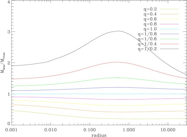
We plot the ratio $M_{\rm kin}(r;q)/M_{\rm true}(r;q)$ as a function of radius for various values of the axis ratio $q$ on the middle panel of Fig. 6. Here again projection effects can be huge for extreme values of $q$. Unfortunately, $M_{\rm kin}(r;q)$ depends on the profile of tracers $\nu(r)$ and the details of this figure cannot be representative of a general oblate/prolate NFW halo. For instance the bump at $r\lesssim 1$ is due to our assumed density of tracers which here corresponds to our model of MS2137. However, departs between $M_{\rm kin}(r;q)$ and $M_{\rm true}$ are always important for high $q$ or $1/q$.

4.3 Projection effect on X-rays

Similarly, we calculate the perturbation of asphericity on X-rays mass estimates. As compared to lensing or dynamics the effect is expected to be weaker since the gravitational potential is systematically rounder than the mass. For simplicity we assume that the gas (with density $\rho_{g}$) is isothermal and in hydrostatic equilibrium.

We have $\rho_{g}\propto\exp[-\Psi/V_{0}^{2}]$ with $V_{0}^{2}=kT/\mu m_{p}$. The X-rays surface brightness of the optically thin gas distribution is

$$S_{X}(R)\propto\int\exp[-2\Psi(R,z)/V_{0}^{2}]{\rm d}z\,,$$ (18)

with $\Psi(R,z)$ given by (14a). Here again, when interpreting this surface brightness distribution as arising from a spherically symmetric system, one will deproject $S_{X}(R)$, obtain a biased gas density $\rho_{g}$ and use it in the following equation to obtain the biased mass profile $M_{\rm X}(r)$.

$$M_{\rm X}(r)=-\frac{V_{0}^{2}r}{G}\frac{{\rm d}\ln\rho_{g}}{{\rm d}\ln r}\,.$$ (19)

We plot the ratio $M_{\rm X}(r;q)/M_{\rm true}(r;q)$ as a function of radius for various values of the axis ratio $q$ on the bottom panel of Fig. 6. As expected $M_{\rm X}(r;q)/M_{\rm true}(r;q)$ exhibits much less scatter about unity as compared to the two previous mass estimates. The asymptotic divergence at very large scales ($r\gtrsim 10$) is a numerical artefact of our crude deprojection algorithm.

Figure 6: Radial behavior of ratio between mass estimates for various values of the axis ratio $q=0.2,0.4,0.6,0.8,1.,1/0.8,1/0.6,1/0.4,1/0.2$.   Top Panel: Ratio $M_{\rm lens}(r;q)/M_{\rm true}(r;q)$.    Middle Panel: Ratio $M_{\rm kin}(r;q)/M_{\rm true}(r;q)$.    Bottom Panel: Ratio $M_{\rm X}(r;q)/M_{\rm true}(r;q)$. In this latter case, one can see much lower values whatever the axis ratio. The asymptotic behavior is slightly affected by numerical instability for $r\gtrsim 10$ and extreme values of $q$.

4.4 Comments and application to MS2137

Fig. 6 clearly shows that moderate values of the axis ratio $q$ can lead to strong discrepancies between 2D and 3D mass estimates or between lensing and X-rays or stellar kinematics.

It is difficult to fully characterize the ratio $M_{\rm lens}(r;q)/M_{\rm kin}(r;q)$ because it depends on the distribution of tracers $\nu(R,z)$ and is severely sensitive to the orientation of the axis ratio relative to the line of sight. Therefore a direct comparison between lensing and dynamical mass estimates is hazardous. $M_{\rm lens}(r;q)/M_{\rm kin}(r;q)$ can have a different radial behavior as a function of radius for a given axis ratio. It can be either greater of less than unity.

Comparing lensing and X-rays mass estimates is easier since the X-rays mass estimate is less sensitive to projection effects. In this respect $M_{\rm lens}(r;q)/M_{\rm X}(r;q)$ will systematically be $>1$ (resp. $<1$) for prolate (resp. oblate) halos with a well known radial behavior.

In the case of MS2137, a prolate halo with $q\sim 0.4$ could well explain most discrepancies between our best fit models and the results of Sa04 and Al01. A prolate halo aligned toward the line of sight is a natural explanation for the high concentration parameter we found $c=11.73\pm 0.55$ and may also explain the high concentrations $c\approx 22$ in CL0024 (Kneib et al. 2003) and $c=13.7^{+1.4}_{-1.1}$ in A1689 (Broadhurst et al. 2005). Recently, Oguri et al. (2005) have investigated the effect of triaxiality in A1689 and have similar conclusions as well as Clowe et al. (2004) who studied numerical simulations (see also Piffaretti et al. 2003).

At this level, it is not possible to simply refine the modelling of MS2137, since our prolate model is idealized. It should be triaxial and/or not perfectly aligned with the line of sight just because the projected density profile is elliptical. However the hypothesis of a projected triaxial halo also provides a direct explanation for the misalignment between the projected diffuse stellar component of the cD and the projected dark matter halo $\Delta\psi=13.0\pm 0.5$ deg. Binney (1985) and Romanowsky & Kochanek (1998) give the necessary formalism to infer the position angle and projected ellipticity of both dark and luminous halos from their tridimensional triaxial shape and orientation. The information that can be derived from the geometry of projected light and dark matter densities is detailed in appendix B. Basically, these independent constraints give the following results for the orientation $\theta$ (polar angle of the major axis with respect to the line of sight), the minor axis ratios $c_{\rm DM}$ and $c_{*}$ of dark matter and stellar components respectively: $\theta=27.4\pm 5.1$, $c_{\rm DM}=0.55\pm 0.08$, and $c_{*}=0.52\pm 0.12$. It is remarquable that this geometrical information is fairly consistent with the value of $c_{\rm DM}\sim 0.4$ and a perfect alignement ($\theta=0$) we assumed to explain the mass discrepancies.

There is sufficient material to be convinced that no simple coupling between 2D and 3D mass estimates is possible. Consequently, we expect that most of the previous analyses based on such a coupling should be considered with caution, either in terms of significance or in terms of possibly biased results.

5 Discrepancies : an expected general trend

The aim of this section is to predict the statistics of such mass discrepancies between lensing and any other mass estimate which is not much sensitive to asphericity effect like X-rays. Let us now consider a more general situation with a triaxial halo $\rho(m)$ where $m^{2}=x^{2}+y^{2}/b^{2}+z^{2}/c^{2}$ with $0<b<c\leq 1$ and an orientation relative to the line of sight parameterized by the polar angles $(\theta,\phi)$ or the unit vector $\@vec{n}$.

The mass within the sphere of radius $r$ is independent on the halo orientation and reads

$$M_{\rm true}(r;b,c)=\frac{1}{4\pi}\int_{0}^{2\pi}{\rm d}\varphi\int_{0}^{\pi}\sin\vartheta{\rm d}\vartheta\,\frac{M_{3}(\nu r;1,1)}{\nu^{3}}\,,$$ (20)

with $\nu^{2}=\sin^{2}\vartheta\left(\sin^{2}\varphi\,/b^{2}+\cos^{2}\varphi\,/c^{2}\right)+\cos^{2}\vartheta$ and again $M_{\rm true}(R;1,1)$ is simply the mass within radius $r$ for a spherically symmetric halo.

The mass $M_{2}$ within cylinder of radius $r$ will depend on their axis ratios and the orientation $\@vec{n}$ but the system is equivalent to an elliptical projected mass distribution with axis ratio $\tilde{q}$ and position angle $\psi$. Thus we can express $M_{2}$ as:

$$M_{2}(r;b,c,\@vec{n})=\frac{\tilde{q}_{x}^{2}}{\sqrt{f}}\int_{0}^{2\pi}\frac{{\rm d}\varphi}{2\pi}\frac{M_{2}(\tau r/\tilde{q}_{x},1)}{\tau^{2}}\,$$ (21)

where $\tau^{2}=\sin^{2}\varphi+\cos^{2}\varphi/\tilde{q}^{2}$ and $\tilde{q}$, $\tilde{q}_{x}$ and $f$ are given by Eqs. (36) in appendix B. They depend on the intrinsic axis ratios and orientation. $M_{2}(r;1,1)$ is simply the cylindric mass within radius $r$ for a spherically symmetric halo.

As before, an observer measuring the 3D mass profile within radius $r$ will find a different normalization as compared to an observer interested in the cylindric mass of radius $r$. They will differ by a factor

$$\eta(R;b,c,\@vec{n})=\frac{M_{2}(r;b,c,\@vec{n})/M_{2}(r;1,1)}{M_{\rm true}(r;b,c)/M_{\rm true}(r;1,1)}\,.$$ (22)

We can now calculate the statistical properties of this ratio by averaging over the $b$ and $c$ PDFs of Jing & Suto (2002) given by (37) and the orientation of the major axis (assumed isotropic). This can be expressed as :

$$p_{R}(\eta)=\frac{1}{4\pi}\int_{0}^{1}{\rm d}c\,p(c)\int_{0}^{1}{\rm d}b\,p(b|c)\\ \int_{0}^{\pi}\sin\theta{\rm d}\theta\,\int_{0}^{2\pi}{\rm d}\phi\,\delta\left[\eta-\eta(R;c,b,\@vec{n})\right]\;.$$ (23)

Figure 7: Upper panel : Distribution for the mass ratio $\eta$ for three different radii $r=0.03$ (the broader black curve), $r=0.3$ (the intermediate red curve) and $r=3.0$ (the narrower green curve). At small scales, the distribution is broad and clearly not centered on $\eta=1$, leading to unreliable direct normalization between 2D and 3D mass estimates like in strong lensing and X-rays/stellar dynamics comparisons. With increasing radius ($r\gtrsim 3.0$), departs significantly vanish and explain the overall agreement between large scale weak lensing and X-rays mass estimates.   Lower panel : Mean (thick black curve) and 68.3, 95.4 and 99.7 % quantiles (thin red, blue and magenta curves respectively) of the $\eta$ distribution as a function of radius.

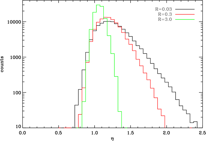
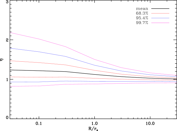
We plot on the upper panel of Fig. 7 the distribution of $\eta$ for three fiducial values of $R=0.03,0.3$ and $3$ which are relevant for strong lensing/stellar dynamics, strong lensing/X-rays and weak lensing/X-rays comparisons respectively. We clearly see a broad, shifted and skewed distribution which converges toward unity with increasing radius. However, at small scales, the median value of $\eta$ is not unity and readily extends toward high values $\eta\gtrsim 1.5$. Typically $\eta=1.24^{+0.23}_{-0.18}$ (resp. $1.19^{+0.17}_{-0.14}$, $1.07\pm 0.06$) for $R=0.03$ (resp. $0.3$, $3.0$). Thus, important departs between $M_{2}$ and $M_{\rm true}$ are naturally expected if halos are effectively triaxial.

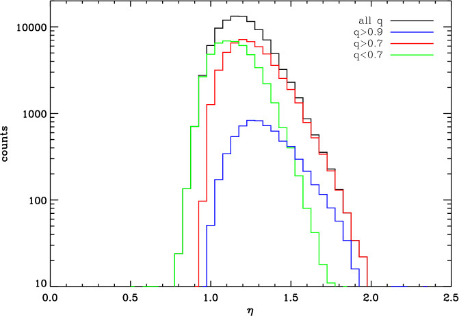
Moreover, there must be a correlation between the observed projected axis ratio $q$ and $\eta$ since the apparently rounder halos are likely to be elongated along the line of sight. This effect can be seen on Fig. 8 where we plot the conditional PDFs $p(\eta)$, $p(\eta|q>0.9)$, $p(\eta|q>0.7)$ and $p(\eta|q<0.7)$ for a radius $R=0.3$. The highest values of $\eta$ are due to the roundest projected halos. For instance, given $q>0.7$ we have $\eta=1.25^{+0.17}_{-0.13}$.

Figure 8: For $r=0.3$, we show the dependence of $\eta$ on the projected axis ratio $q$. The conditional PDFs $p(\eta|q>0.9)$ (blue) $p(\eta|q>0.7)$ (red) and $p(\eta|q<0.7)$ (green) are compared to the overall distribution $p(\eta)$ (black). The rounder the halo is, the more likely is the major axis of the halo oriented toward the line of sight and the higher is $\eta$.

Finally projection effects of triaxial halos have the interesting properties to explain the fact that weak lensing and X-rays measurements generally match since $\eta\sim 1$ for $r\gtrsim$ a few $r_{s}$. Likewise the general trend for strong lensing mass estimates to generally be greater (by a factor of $1-3$) than X-rays since they occur at scales $0.1\lesssim r\lesssim 1$ (Allen et al. 2001; Wu 2000). The relative normalization between lensing and stellar kinematics is more complex and cannot be representated by the $\eta$ statistic. However we expect a similar scatter and a strong dependence on the major axis orientation.

6 Discussion & Conclusion

Regarding the particular case of MS2137, using a detailed modelling of both strong and weak lensing data, we have shown that the dark matter density profile must be close to NFW. See also (Miralda-Escudé 1995; Bartelmann 1996; Gavazzi et al. 2003; Bartelmann & Meneghetti 2004; Dalal & Keeton 2003) for similar conclusions. We have explained the reason why the Sa04 lens model is inconsistent with lensing data (radial arc counter image, weak lensing…). We have highlighted a possible discrepancy between our lens model and other mass estimates from stellar kinematics in the central cD galaxy and X-rays.

We have undertaken a thorough dynamical analysis of the line-of-sight velocity distribution of stars in the cD in order to check whether or not departs from gaussianity may explain the relative inconsistency between our lens models and stellar kinematics. The effect of non-gaussian aborption lines is to slightly lower ($\sim 15\%$) the measured velocity dispersion estimates of Sa04 but does not greatly improve the agreement between our lens model and the bias-corrected data. Moreover such a bias cannot explain the disagreement between our lens model and Al01 X-rays mass estimates. This latter 3D mass estimates turns out to be consistent with stellar dynamics, showing that there must exist some problem in the relative normalization of 2D and 3D mass estimates.

These discrepancies can be alleviated if one considers the possibility of departs from spherical symmetry for the dark matter and stellar components. More precisely, we have shown that a prolate halo with its major axis oriented close to the line of sight and an axis ratio $\sim 0.4$ is likely to explain the discrepancies. This hypothesis is supported by the misalignement ($\Delta\psi\sim 13^{\circ}$) between projected DM and stellar distributions.

Furthermore such a geometrical configuration well explains the concentration parameter we infer from lensing analysis $c=11.73\pm 0.55$. A prefered elongated halo toward the LOS boosts lensing efficiency (Bartelmann 1995; Oguri et al. 2003; Clowe et al. 2004) and may explain the high concentration of some strong lensing clusters (Kneib et al. 2003; Broadhurst et al. 2005; Oguri et al. 2005; Hennawi et al. 2005).

We have shown that triaxiality is a general problem that hampers any attempt to simply couple 2D and 3D mass estimates assuming spherical symmetry. Once projected, triaxial halos are elliptical and lens modelling is able to take ellipticity into account. Usually dynamical or X-rays analyses do not fully incorporate such a complexity. This should be an important work to do before comparison to (or coupling with) lensing. In Sect. 5, we have assumed the statistical distribution of axis ratios proposed by Jing & Suto (2002) in order to calculate the mass $M_{2}(r)$ within cylinder of radius $r$ and the mass $M_{\rm true}(r)$ within the sphere of same radius. The difference is important and can lead to a significant discrepancy in the relative normalization between 2D and 3D mass estimates.

The statistic of $\eta(r)$ shows that, at small scales $R<1$, in average a systematic depart from unity is expected for $\eta$ with an important scatter and skewness toward high values of $\eta$. Therefore the relative normalization at small scales is biased and highly uncertain if one neglects projection effects. At larger scales, the distribution of $\eta$ converges to unity and explains why weak lensing mass estimates are generally in better agreement with X-rays or dynamics of galaxies in clusters (e.g.  Allen 1998; Wu 2000; Arabadjis et al. 2004). Similarly, the coupling between stellar kinematics and strong lensing at clusters scales (Sand et al. 2002, 2004) or at galaxies scales (e.g.  Koopmans & Treu 2002; Treu & Koopmans 2004; Rusin et al. 2003) may be oversimplistic since they do not take asphericity into account. First, the mean value $\eta\sim 1.2$ for $r\lesssim 0.3r_{s}$ leads to a expected systematic bias, but also the $\sim 20\%$ scatter in the distribution of $\eta$ will increase the uncertainty in the mass normalization and prevent the appealing temptation to couple these independent mass estimates.

In conclusion, the density profile of the dark matter halo of MS2137-23 is well consistent with NFW and previous claimed discrepancies may be due to the spherical symmetry assumption. Indeed, it turns out that when coupling lensing to other mass estimates we cannot avoid a detailed (and cumbersome) 3D triaxial modelling of X-rays and dynamical properties. It is worth noticing that such a level of refinement is already achieved in lensing studies that assume elliptical symmetry. The triaxiality of dark matter halos (and stellar components) is a major concern for joint modelling and should systematically be taken into account for future analyses. As well, it is possible that X-rays or optically selected clusters are biased toward elongated configurations, leading to an overefficiency for lensing. The increasing precision of observations makes the assumption of spherical symmetry abusive. Since clusters of galaxies are often seen as an important cosmological probe. It is important to better characterize their properties (mass, temperature, shape, abundance…) with realistic triaxial symmetries.

Appendix A LOSVD of stars in the BCG

The aim of this analysis is to derive the whole line-of-sight velocity distribution (LOSVD) of stars from the gravitational potential $\Phi$. $r$ denotes the three-dimensional radial coordinate whereas $R$ is the 2D projected radius and the density of tracers $\rho_{*}(r)$ (the luminosity density). We assume that the distribution function DF $f(\@vec{r},\@vec{v})$ can be modeled by Osipkov-Merritt (Osipkov 1979; Merritt 1985) distribution functions (DF) which depend on the reduced energy ${\mathcal{E}}=\Psi(r)-v^{2}/2$ and angular momentum $L=rv\sin\zeta$ through the variable

$$Q={\mathcal{E}}-\frac{L^{2}}{2r_{a}^{2}}=\Psi(r)-\frac{v^{2}}{2}\left(1+\frac{r^{2}}{r_{a}^{2}}\sin^{2}\zeta\right)\;.$$ (24)

In these equations $\Psi(r)=\Phi(r_{\rm max})-\Phi(r)$ is the reduced potential, $\zeta$ is the polar angle of the velocity direction with respect to $\@vec{r}$ and $r_{\rm max}$ is the outermost radius at which a particle is bound to the system, i.e. satisfying ${\mathcal{E}}\geq 0$. Otherwise specified, we set $r_{\rm max}=2\,h_{\rm 70}^{-1}\,{\rm Mpc}$ in the following. $r_{a}$ is the anisotropy radius. Orbits are nearly isotropic for $r_{a}\rightarrow\infty$ and nearly radial for $r>r_{a}$.

For Osipkov-Merritt models, the DF $f(Q)$ can directly be calculated, through the Eddington formula (Binney & Tremaine 1987)

$$f(Q)=\frac{1}{\sqrt{8}\pi^{2}}\left[\int_{0}^{Q}\frac{{\rm d}^{2}\tilde{\rho}_{*}}{{\rm d}\Psi^{2}}\frac{{\rm d}\Psi}{\sqrt{Q-\Psi}}+\frac{1}{\sqrt{Q}}\left(\frac{{\rm d}\tilde{\rho}_{*}}{{\rm d}\Psi}\right)_{\Psi=0}\right]\;.$$ (25)

where $\tilde{\rho}_{*}=(1+\frac{r^{2}}{r_{a}^{2}})\rho_{*}$.

Once the Eq. (25) numerically integrated, it is possible to derive the LOSVD $p(R,v_{\shortparallel})$ as a function of the projected radius $R$ by integrating over the line of sight coordinate $z$ and over the perpendicular velocity $v_{\perp}$ with $v^{2}=v_{\shortparallel}^{2}+v_{\perp}^{2}$.

$$p(R,v_{\shortparallel})\propto\int_{0}^{z_{\rm m}}{\rm d}z\int_{0}^{v_{\perp,{\rm m}}}v_{\perp}{\rm d}v_{\perp}\>f(Q)\;,$$ (26)

with $z_{\rm m}$ the maximum line-of-sight coordinate for a particle moving at velocity $v$ located at the projected radius $R$ and satisfying $\Psi(\sqrt{R^{2}+z_{\rm m}^{2}})=v^{2}/2$. In the isotropic case, Eq. (26) can be simplified :

$$p_{\rm iso}(R,v_{\shortparallel})=2\pi\int_{v_{\shortparallel}^{2}}^{2\Psi(R)}{\rm d}v^{2}\int_{0}^{z_{\rm m}(v)}{\rm d}z\>f({\mathcal{E}})\;,$$ (27)

and a numerical integration is rather fast. However, in the general case, this is not possible and we present in the following a much faster Monte-Carlo technique.

The integration of Eq. (26) is done by randomly sampling the distribution function with a large number $N$ of stars. Since the stellar density profile is known to a scaling mass-to-light ratio, one can assign a radius $r$ to each star according to the cumulative Hernquist stellar mass profile $M_{*}(r)=M_{*}\left(\frac{r}{r+r_{s*}}\right)^{2}$. Each radius $r_{i}$ can be projected onto the plane of sky yielding $\@vec{R}_{i}$ and $z_{i}$, the line of sight coordinate as before. At this point, it is trivial to incorporate the smearing due to observational conditions like seeing by adding a random displacement $\@vec{R}_{i}\rightarrow\@vec{R}_{i}+\@vec{\delta R}_{i}$. Similarly, if the slit width $\Delta$ is negligible $R_{i}=|\@vec{R}_{i}|$ can be identified to the position along the slit, otherwise, it is straightforward to split $\@vec{R}_{i}$ into $(x_{i},y_{i})$, only consider those points satisfying $2|y_{i}|\leq\Delta$ and then identify $x_{i}$ as the position along the slit. This is the situation we shall consider in the following.

This spatial sampling of the DF is thus independent of the potential $\Psi$ or the anisotropy radius $r_{a}$ and can be stored for further calculation. For a given $\Psi(r)$ and $r_{a}$, one must solve Eq. (25), assign a velocity $v$ and a velocity orientation $\Omega$ using the calculated DF $f(Q)$. This sampling is done with acceptance-rejection technics (e.g.  Press et al. 1992). See also Kuijken & Dubinski (1994) or Kazantzidis et al. (2004) for similar applications. We can write the conditional PDFs for the polar angle $\zeta$ and $Q$ at radius $r$ :

$$\begin{split}p(\zeta|r)=&\frac{1}{2}\frac{\sin\zeta}{\left(1+\frac{r^{2}}{r_{a}^{2}}\sin^{2}\zeta\right)^{3/2}}\\ p(Q|r)\propto&f(Q)\sqrt{2(\Psi(r)-Q)}\;.\end{split}$$ (28)

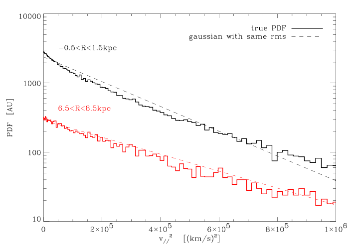
Hence each star has a position $x_{i}$ and a line-of-sight velocity $v_{\shortparallel,i}$. It is now possible to calculate $p(R,v_{\shortparallel})$ and the associated velocity dispersion $\sigma_{\rm los}(R)=\sqrt{\overline{v_{\shortparallel}^{2}}}$ and kurtosis $\kappa(R)=\frac{\overline{v_{\shortparallel}^{4}}}{\sigma_{\rm los}^{4}}-3$, respectively related to the second and forth order moments of $p(R,v_{\shortparallel})$.

We now compute the LOSVD deduced from the best fit NFW model of MS2137 and compare the inferred velocity dispersion to the measurements of Sa04. We assume the same observational conditions i.e. a slit width $\Delta=1.25\arcsec\simeq 5.8\,h_{\rm 70}^{-1}\,{\rm kpc}$ and a gaussian seeing $0.6\arcsec=2.8\,h_{\rm 70}^{-1}\,{\rm kpc}$ FWHM. These data were obtained by assuming Gaussian absorption lines. van der Marel & Franx (1993) showed that departs from Gaussianity imply a bias in any velocity dispersion measurement. To the first order, the biased pseudo-velocity dispersion $\sigma_{\rm h_{4}}$ reads:

$$\sigma_{\rm h_{4}}=\frac{\sigma_{\rm los}}{1+\kappa/8}\;.$$ (29)

In the Gaussian case ($\kappa=0$), $\sigma_{\rm h_{4}}$ reduces to $\sigma_{\rm los}$.

Fig. 9 shows the LOSVD as a function of the line-of-sight velocity $v_{\shortparallel}$ for the innermost and outermost radial bins of Sa04. Departs from Gaussianity are visible close to the center and decrease with increasing radius. Therefore, the velocity bias changes with projected radius as can be seen on the top panel of Fig. 5, in which we plot $\sigma_{\rm los}(R)$ and $\sigma_{\rm h_{4}}(R)$ for two values of the anisotropy radius $r_{a}=\infty$ and $r_{a}=10\,h_{\rm 70}^{-1}\,{\rm kpc}$.

Figure 9: Line-of-sight velocity probability distribution for stars with a projected radius in the innermost $-0.5<R<1.5\,h_{\rm 70}^{-1}\,{\rm kpc}$ (the upper black histogram) and outermost bins $6.5<R<8.5\,h_{\rm 70}^{-1}\,{\rm kpc}$ (the lower red histogram)of Sa04. In each case, we plot a gaussian distribution with the same dispersion for comparison. One can see non-gaussian tails for innermost stars. In this exemple, we consider the the best fit NFW model of Sect. 2.3 and orbits are isotropic.

Appendix B Further evidence for triaxiality

In this section we follow the formalism of Binney (1985) and Romanowsky & Kochanek (1998) and calculate the orientation and axis ratio of a projected triaxial distribution as a function of its intrinsinc 3D axis ratios $0\leq c\leq b\leq 1$ such that the density $\rho(\@vec{r})=\rho(m)$ with $m^{2}=x^{2}+y^{2}/b^{2}+z^{2}/c^{2}$. We express the orientation of the minor axis with the polar angles $(\theta,\phi)$ relative to the line of sight. The projected density reads :

$$\Sigma(x,y)=\frac{2}{\sqrt{f}}\int_{0}^{\infty}\rho(u^{2}+m^{2})\,{\rm d}u\;,$$ (30)

where

$$f=\sin^{2}\theta\left(\cos^{2}\phi+\frac{\sin^{2}\phi}{b^{2}}\right)+\frac{\cos^{2}\theta}{c^{2}}\;,$$ (31)

$$m^{2}=\frac{1}{f}\left(Ax^{2}+Bxy+Cy^{2}\right)\;,$$ (32)

$$A=\frac{\cos^{2}\theta}{c^{2}}\left(\sin^{2}\phi+\frac{\cos^{2}\phi}{b^{2}}\right)+\frac{\sin^{2}\theta}{b^{2}}\;,$$ (33)

$$B=\cos\theta\sin 2\phi\,\left(1-1/b^{2}\right)\frac{1}{c^{2}}\;,$$ (34)

$$C=\left(\frac{\sin^{2}\phi}{b^{2}}+\cos^{2}\phi\right)\frac{1}{c^{2}}\;.$$ (35)

The projected distribution is elliptical with an axis ratio $\tilde{q}$ and a position angle $\psi$ given by :

$$\tilde{q}_{x/y}^{2}= \frac{2f}{A+C\mp\sqrt{B^{2}+(A-C)^{2}}}\;,$$ (36a)

$$\tilde{q}= \tilde{q}_{y}/\tilde{q}_{x}\;,$$ (36b)

$$\tan 2\psi= \frac{B}{A-C}\;.$$ (36c)

These equations are verified by the dark matter and the stellar components which have their own axis ratios $c_{\rm DM}$, $b_{\rm DM}$, $c_{*}$ and $b_{*}$ but their principal axes are assumed to match. Generally, different values of $c_{i}$ and $b_{i}$ lead to different values of $\tilde{q}_{i}$ and $\psi_{i}$. This is what we observe in MS2137 where the light satisfies $\tilde{q}_{*}=0.83\pm 0.12$, $\psi_{*}=(18\pm 1)\,\mathrm{deg}$ and our NFW lens modelling yields $\tilde{q}_{\rm DM}=0.750\pm 0.005$ and $\psi_{\rm DM}=(4.90\pm 0.15)$ deg. Hence we can infer the parameters $\theta,\phi,c_{\rm DM},b_{\rm DM},c_{*},b*$ from these constraints and some additional priors since the problem is underconstrained. We can use the axis ratio distribution found in cosmological simulations by Jing & Suto (2002):

$$p(c)= \frac{1}{\sqrt{2\pi}\sigma_{c}}\exp\left(-\frac{(c-\bar{c})^{2}}{2\sigma_{c}^{2}}\right)\;,$$ (37a)

$$p(b|c)= \frac{3}{2(1-\max(c,1/2))}\left[1-\left(\frac{2b-1-\max(c,1/2)}{1-\max(c,1/2)}\right)^{2}\right]\;,$$ (37b)

with $\sigma_{c}\sim 0.113$ and $\bar{c}\sim 0.54$. In addition, since the number of constraints is not sufficient we force the intermediate axis ratios $b_{*}$ and $b_{\rm DM}$ to be equal to the most probable value. In other word, we have

$$p(b|c)=\delta\left(b-\frac{1+\max(1/2,c)}{2}\right)\;.$$ (38)

The best fit with priors yields : $\theta=27.4\pm 5.1$, $c_{\rm DM}=0.55\pm 0.08$ and $c_{*}=0.52\pm 0.12$. This analysis gives strong indications on the reliability of triaxial dark matter and stellar distribution with the major axis relatively close to the line-of-sight and a value of $c_{\rm DM}$ close to that inferred to explain the discrepancy between 2D and 3D mass estimates in Sect. 4.1.