The radial distribution of magnetic helicity in the solar convective zone: observations and dynamo theory
Abstract
We continue our attempt to connect observational data on current helicity in solar active regions with solar dynamo models. In addition to our previous results about temporal and latitudinal distributions of current helicity (Kleeorin et al. 2003), we argue that some information concerning the radial profile of the current helicity averaged over time and latitude can be extracted from the available observations. The main feature of this distribution can be presented as follows. Both shallow and deep active regions demonstrate a clear dominance of one sign of current helicity in a given hemisphere during the whole cycle. Broadly speaking, current helicity has opposite polarities in the Northern and Southern hemispheres, although there are some active regions that violate this polarity rule. The relative number of active regions violating the polarity rule is significantly higher for deeper active regions. A separation of active regions into ‘shallow’, ‘middle’ and ‘deep’ is made by comparing their rotation rate and the helioseismic rotation law. We use a version of Parker’s dynamo model in two spatial dimensions, that employs a nonlinearity based on magnetic helicity conservation arguments. The predictions of this model about the radial distribution of solar current helicity appear to be in remarkable agreement with the available observational data; in particular the relative volume occupied by the current helicity of ”wrong” sign grows significantly with the depth.
keywords:
Sun: magnetic fields – Sun: activity – Sun: interior1 Introduction
The solar 22-year activity cycle is thought to be a manifestation of dynamo action somewhere inside the solar convective zone or even in the overshoot layer. The solar differential rotation acts as a driver of the solar dynamo, generating a toroidal magnetic field from an existing poloidal magnetic field. The other dynamo driver, required to transform toroidal magnetic field into poloidal and so to close the chain of self-excitation, is thought to be what is commonly known as the -effect, i.e. a specific feature of convective flows in a rotating body. It was E. Parker who suggested as early as 1955 that cyclonic motions in the solar convective zone produce a mean (large-scale) poloidal magnetic field from a mean toroidal magnetic field. Ten years later, Steenbeck, Krause & Rädler developed a theory of this process, calling it the -effect (see Krause & Rädler 1980). A physical feature of the -effect in the form discussed at this stage is that the action of the Coriolis force on the convective vortices results in a domination of right-handed vortices in the Northern solar hemisphere and, correspondingly, left-handed vortices in the Southern. A non-vanishing difference between vortices with right and left helicities in a given hemisphere provides the required conversion of toroidal magnetic field to poloidal.
Parker (1955) demonstrated that the scheme briefly discussed above leads to the self-excitation of a wave of magnetic field (the so-called dynamo wave). A suitable choice of the differential rotation shear and mean helicity of solar convection in, say, the Northern hemisphere leads to a dynamo wave whose shape mimics remarkably that of the solar butterfly diagram. The simplest order of magnitude estimates for the dynamo governing parameters results in an estimate for the cycle length which is about 10 times shorter then the real solar cycle – this seems reasonable for this obviously oversimplified model.
Until now the above scheme for the solar dynamo, known as the Parker migratory dynamo, has remained the basis of most dynamo models for solar and stellar dynamo activity. Of course, present day solar dynamo models include achievements of helioseismology, effects of meridional circulations and various other features of solar MHD. As a result, these dynamo models are much richer and, in principle at least, closer to the real Sun then the simple Parker model. Nevertheless, although these more sophisticated models can reproduce many specific details, some points remain as obscure now as in 1955 (for recent reviews, see Ossendrijver 2003; Brandenburg & Subramanian 2004).
Note that the -effect remained for several decades a theoretical concept only. It is deeply associated with the helicity of rotating turbulence and arises from averaging Maxwell’s equations over the ensemble of rotating vortices. For a long time, there was no evidence available to support the -effect from either astronomical observations or from laboratory MHD experiments. Obviously, such a situation makes the basis of solar dynamo theory rather unsatisfactory and even shaky.
In the last decade, some basic progress here has been made and the first observational data of physical quantities associated with the -effect are now available. The fundamental point is that the -effect includes two contributions (Pouquet et al. 1976), an hydrodynamical contribution as discussed above () associated with helicity of convective vortices, and also a contribution from the helicity of the magnetic field itself (). The hydrodynamic helicity is determined by a correlation between the convective velocity and its vorticity, i.e. , and so its observational determination requires knowledge of all three components of velocity while the Doppler effect gives a line-of-sight velocity component only. The magnetic part of the -effect, , can be related to what has become known as the current helicity, proportional to , where is the small-scale magnetic field. Because Zeeman splitting provides information concerning all 3 components of , appears to be more accessible for observational determination than (Seehafer 1990). As a result, the first observations to be made relate to the current helicity in active regions on the solar surface (Pevtsov et al. 1994, 1995; Zhang & Bao 1998, 1999; Longcope et al. 1998).
Such observational findings about the current helicity on the solar surface can be related to theoretical results in dynamo theory, where the concept of the magnetic part of -effect has been developed into a theory of dynamo saturation through . Kleeorin & Ruzmaikin (1982) and Kleeorin & Rogachevskii (1999) suggested a governing equation for which describes the time evolution of the -effect. Together with the mean-field dynamo equations, this equation has solutions in the form of a propagating dynamo wave which amplitude is steady in time (Kleeorin et al. 1995; Covas et al. 1998; Blackman & Brandenburg 2002).
Kleeorin et al. (2003) discussed a link between the observational and theoretical findings outlined above. They concluded that the accumulated observational knowledge is sufficient to follow the temporal evolution during one solar cycle of current helicity averaged over a given hemisphere or the latitudinal distribution of current helicity averaged over one solar cycle. Existing ideas concerning the nonlinear solar dynamo saturated by the magnetic part of the -effect provide a theoretical prediction of the corresponding quantities. These demonstrate a general agreement with observations and provide a possibility of fitting the governing parameters of the solar dynamo by observational data.
Here we present an extension of the approach of the paper of Kleeorin et al. (2003). First of all, we discuss the extent to which the solar helicity data can be used to understand the radial dependence of solar magnetic helicity and the corresponding dynamo activity. An initial step in this direction was made by Kuzanyan et al. (2003) who separated the database of active regions for which the helicity data are available into subsets corresponding to shallow, middle and deep active regions, according to their rotation rate. Of course, a substantial part of the data cannot be so classified. After averaging magnetic helicity data over the subsets, we obtain quantities which can be compared with the theoretical data averaged over the three radial ranges.
This approach is to some extent similar to the studies of the solar rotation curve using the sunspot data associated with various types of sunspots. Following the remarkable advances in helioseismology such reconstructions now look rather archaic (this is why we refer here only to the single paper, Collin et al. (1995), in which one of the authors participated). However, at this preliminary stage of solar helicity studies, a similar approach appears to be reasonable.
The other topic to be addressed here is a plausible improvement of the governing equation for the magnetic helicity. The point is that the dynamo saturation by a magnetic contribution to the -effect is necessarily combined with a modification of the turbulent diffusivity and other transport coefficients. For the sake of simplicity, these effects were ignored in our first paper (Kleeorin et al. 2003). Now we restore these terms in order to investigate their possible contribution, and to produce a more fully self-consistent model.
Obviously, our model is still simplified and does not include many important features of solar activity. In particular we do not address the problem of the storage of magnetic fields and the formation of flux tubes in the overshoot layer near the bottom of the convective zone (see, e.g., Spiegel & Weiss 1980; Tobias et al. 2001; Tobias & Hughes 2004; Brandenburg 2005, and references therein).
2 Data on current helicity obtained at the Huairou Solar Observatory Station
Our research is based on the data on current helicity accumulated during 10 successive years (1988-97) of observations at the Huairou Solar Observatory Station of the National Astronomical Observatories of China (Bao and Zhang 1998), which were further processed by Zhang et al. (2002). The description of the observational procedure and the basic ideas of data processing can be found in Kleeorin et al. (2003) and references therein. The total available sampling that we used contains data of 410 active regions.
Following Kuzanyan et al. (2003) we divide the active region into 4 groups, i.e. shallow, middle and deep active regions, as well as a group for which the depth cannot be estimated satisfactorily (Table 1). The separation of the active regions into three groups is based on the result of helioseismology (Schou et al. 1998) that the angular rotation rate growth monotonically with radius at least for the domain between fractional radii 0.65 and 0.95 and latitudes below 30-35∘ (for details see Kuzanyan et al. 2003).
The Solar Geophysical Data records, which can be obtained from the NOAA (USAF-MWL) database, provide us with several tens of longitudinal locations (in terms of the Carrington coordinate system) for each active region under investigation, for several consequent days. Therefore, we attempt to calculate partial, or “individual”, angular rotation rates with respect to the Carrington rotation. For some active regions we can find a certain trend in the evolution of their Carrington coordinates with time. From the complete sampling of the data, which contain 410 active regions, we select subsamples for which this trend in Carrington longitude versus time has significant correlation. We determined the subsamples for which the correlation coefficient is greater than 0.5 and 0.6 respectively. These samples contain 178 and 134 active regions (or and of the available data), respectively.
Given an “individual” angular rotation rate for each active region we can identify them with certain effective depths. Using a particular analytical approximation of the solar rotation curve (see Kuzanyan et al. 2003), the active regions with known individual angular rotation were separated into three groups. The individual rotation rates in the first group fall into the range covered by the analytical approximation for the radial range , for the second group the bound is , and for the third group. These groups were labelled as deep, middle and shallow. Notice, that the internal rotation of the solar convective zone above approximately fractional radius 0.94 is slower than in the zone below, and so we disregarded this sub-surface layer. We stress that the above bounds were chosen rather arbitrarily and the details of trends in the current helicity properties with respect to depth can hardly be considered quantitatively. The active regions appear to be distributed between the upper and lower layers approximately equally, while very few occur within the middle layer (Kuzanyan et al. 2003). We will consider separately the upper and lower layers and compare the results of statistical analysis of the data in each of them.
Because the current helicity is expected to be of opposite sign in Northern and Southern hemispheres, we subdivide these groups between the two hemispheres and average the data in each group over all latitudes as well as cycle phases. The result of averaging is given in Table 1 for active regions with identified depth. Here is a depth identifier, with ”s” meaning shallow, ”m” middle and ”d” deep active regions. Because the number of active areas of intermediate depth appears to be quite low, and insufficient to estimate the sign of helicity, we combine quite arbitrarily the data for the middle and deep active regions into a single group, i.e. ”d+m”. is the number of active regions included in each group. For Table 1, we use the threshold . To demonstrate the stability of the selection procedure to the threshold value, we give in Table 2 similar results for the threshold value .
| Table 1 | ||||
|---|---|---|---|---|
| Current helicity for active regions | ||||
| binned by depth, threshold Here and | ||||
| below is measured in in units of | ||||
| North | ||||
| s | 47 | 1 | ||
| m | 5 | 1 | ||
| d | 34 | 8 | ||
| d+m | 39 | 9 | ||
| South | ||||
| s | 41 | 5 | ||
| m | 6 | 2 | ||
| d | 38 | 11 | ||
| d+m | 44 | 13 | ||
| Table 2 | ||||
|---|---|---|---|---|
| Current helicity for active regions | ||||
| binned by depth, threshold | ||||
| North | ||||
| s | 33 | 1 | ||
| m | 2 | 1 | ||
| d | 28 | 7 | ||
| d+m | 30 | 8 | ||
| South | ||||
| s | 33 | 4 | ||
| m | 3 | 2 | ||
| d | 29 | 9 | ||
| d+m | 32 | 11 | ||
In agreement with theoretical expectations, the data for are remarkably antisymmetric in respect to the solar equator. Note that the same kind of antisymmetry was recognized in the averaging over latitude or time undertaken in Kleeorin et al. (2003). We note however that there are a significant number of active regions that violate this polarity law. The number of such active regions are given in Tables 1 and 2 as .
We present in Table 3 the averaged values of the helicities of for all 410 active regions for which the observations of helicity are available. These active regions follow the same polarity rule as the active regions with known depth, and again some active regions violate this rule. Their number is given as .
| Table 3 | ||||
|---|---|---|---|---|
| Current helicity for all 410 active regions | ||||
| hemisphere | ||||
| North | 193 | 30 | ||
| South | 217 | 47 | ||
The number of active regions with current helicity that violate the polarity rule can be calculated for both hemispheres (Table 4). Note that it is not appropriate to average the current helicity over both hemispheres because the data in the Northern and Southern hemisphere cancel. We conclude from Table 4 that the deep (and middle) active regions contain several times more cases of parity rule violations than the shallow active regions, and even slightly more then the active regions without definite estimation of depth.
We were unable to recognize any clear trend in the number of active regions violating the polarity rule selected according to latitude or the cycle phase. However we present the relevant data below (Tables 5 and 6).
| Table 4 | |||
|---|---|---|---|
| Number of active region with current | |||
| helicity violating the polarity rule, | |||
| binned by depth, threshold . | |||
| depth | |||
| s | 88 | 6 | |
| d+m | 83 | 22 | |
| Table 5 | |||
|---|---|---|---|
| Number of active region with current | |||
| helicity violating the polarity rule | |||
| ordered by date, threshold . | |||
| years | |||
| 1988-89 | 87 | 23 | |
| 1990-91 | 126 | 20 | |
| 1992-93 | 121 | 18 | |
| 1994-96 | 69 | 13 | |
| Table 6 | |||
| Number of active region with current | |||
| helicity violating the polarity rule, | |||
| ordered by latitude , threshold . | |||
| latitude (degrees) | |||
| 18 | 4 | ||
| 53 | 10 | ||
| 36 | 5 | ||
| 48 | 8 | ||
| 65 | 6 | ||
| 58 | 12 | ||
| 46 | 8 | ||
| 67 | 19 | ||
| 12 | 3 | ||
3 The dynamo model
We use here a dynamo model which is basically an extension of the simplified model of Kleeorin et al. (2003). In particular, the present model includes an explicit radial coordinate and takes into account the curvature of the convective shell, and also quenching of turbulent magnetic diffusivity. We start from the general mean-field dynamo equations (see e.g. Moffatt 1978, Krause & Rädler 1980). Using spherical coordinates we describe an axisymmetric magnetic field by the azimuthal component of magnetic field , and the component of the magnetic potential corresponding to the poloidal field. Following Parker (1955) we consider dynamo action in a convective shell. However we retain a radial dependence of and in the dynamo equations and we do not neglect the curvature of the shell. The equations for and read
| (1) | |||
| (2) |
where
Here we measure lengths in units of the solar radius and time in units of a diffusion time based on the solar radius and the turbulent magnetic diffusivity . When estimating this timescale we use the ‘basic’ (assumed uniform) value of the turbulent magnetic diffusivity, unmodified by the magnetic field.
We consider the fractional radial range , where corresponds to the bottom of the convective zone and corresponds to the solar surface. The ‘convection zone’ proper can be thought of as occupying , with being a tachocline/overshoot region. The rotation law includes radial shear (proportional to ) and a latitudinal dependence (proportional to ).
At the surface we use vacuum boundary conditions on the field, i.e. and the poloidal field fits smoothly onto a potential external field. At the lower boundary, , . At both and , , where is the current helicity (see Eq. (3)).
Of course these equations, although more elaborate than those often used to study the solar cycle, are still oversimplified. However they appear adequate to reproduce the basic qualitative features of solar (and stellar) activity. Taking into account the exploratory nature of the approach, we use the simplest profiles of dynamo generators compatible with symmetry requirements and with producing a magnetic butterfly diagram that is concentrated towards low latitudes (see also Rüdiger & Brandenburg 1995; Moss & Brooke 2000). Thus the unquenched hydrodynamical part of the -effect, and (this determines the sign value of the hydrodynamic effect, see below in Sect. 4). The points and correspond to the North and South poles respectively. See Kleeorin et al. (2003) for further discussion of this approach.
As a new feature of Eqs. (1) and (2), compared with the dynamo model exploited by Kleeorin et al. (2003), we retain here the possibility of including a contribution from the dynamo generated magnetic field in the turbulent diffusion coefficients ( and ), and the meridional circulation ( and ). However we do not consider fully here the role of meridional circulation.
The magnetic field is measured in units of the equipartition field , and the vector potential of the poloidal field is measured in units of . The density is normalized with respect to its value at the bottom of the convective zone, and the basic scales of the turbulent motions and turbulent velocity at the scale are measured in units of their maximum values through the convective zone. Because turbulent diffusivity and -effect depend on the magnetic field, we use their initial values in the limit of very small mean magnetic field to obtain the dimensionless form of the equations. To emphasize this, we do not introduce the dynamo number in an explicit form here however use it below when convenient.
4 The nonlinearities
We present below a model for the nonlinear dynamo saturation. The model is based as far as possible on first principles, and is similar to that used in the derivation of the equations of mean-field electrodynamics by Krause & Rädler (1980). As an important technical point, we used a quasi-Lagrangian approach in the framework of Wiener path integrals to derive the dynamical equation for the evolution of the magnetic helicity including magnetic helicity flux (see Kleeorin & Rogachevskii 1999). We also used the spectral -approximation (Orszag’s third-order closure procedure) to determine the nonlinear mean electromotive force (see Rogachevskii & Kleeorin 2000, 2004). Here we note some important features of the model only.
A key assumption of the model under discussion is the concept of the locally isotropic and weakly inhomogeneous nature of the background MHD turbulence (with a zero mean magnetic field). Because we include large-scale phenomena such as helicity advection, the accuracy of the approximation is limited. In particular, a completely rigorous evaluation of the turbulent diffusion of magnetic helicity is beyond the scope of our model and we allow this quantity to be transported by the turbulent diffusion in the same way as a scalar admixture, i.e. the turbulent diffusion coefficient is determined by the velocity field correlation tensor. In contrast, the nonlinear coefficients of the large-scale magnetic field defining the nonlinear mean electromotive force are determined by the cross-helicity of magnetic () and velocity () fields, i.e. by . The different scalings for these quantities presented below are connected with this fact.
Note that a deeper investigation of the turbulent diffusion of magnetic helicity, as well as of the non-diffusive fluxes of magnetic helicity, looks possible in principle. It would require at least the application of Orszag’s fourth-order closure procedure to derive the magnetic helicity fluxes. However, this generalization would require a much more extended calculation than required to obtain the model considered here. As a substantial body of calculations already have been necessary, it seems very reasonable to clarify the astrophysical consequences of the model now available, before attempting to move on further.
We stress again that the model analyzed is derived, as far as possible, from first principles. The scope of the model is however obviously limited and does not include all possible physical mechanisms which could in principle contribute to dynamo saturation. In particular, we do not include the buoyancy of the magnetic field. Some other limitations are mentioned below. Bearing in mind the natural limitations of the model, we introduce several numerical coefficients multiplying the magnetic helicity fluxes, which we consider to be free parameters of order unity (see Eq. (5) below).
4.1 The -effect
The key idea of the dynamo saturation scenario exploited below (as well as by Kleeorin et al. 2003) is the splitting of the total -effect into its hydrodynamic and magnetic parts, and respectively. The calculation of the magnetic part of the -effect is based on the idea of magnetic helicity conservation and the link between current and magnetic helicities, and gives (see Kleeorin et al. 2000, 2003)
| (3) |
Here and are proportional to the hydrodynamic and current helicities respectively and and are quenching functions. The analytical form of the quenching functions and is given in Appendix A. In contrast to Kleeorin et al. (2003), we consider here the radial helicity profiles in an explicit form and so we keep in Eq. (3) the radial profile of density normalized by the density at the bottom of the convective zone. This factor appears as (for details, see Kleeorin et al. 2003). Based on Baker & Temesvary (1966) and Spruit (1974), we choose for the analytical approximation
| (4) |
where and . Here corresponds to a tenfold change of the density in the solar convective zone, by a factor of about , etc. However in the majority of our investigations we took , but we did also consider cases with .
The equation for is
| (5) |
where , and the flux of the magnetic helicity is chosen in the form
| (6) | |||||
with . Here is the ratio of the solar radius to the basic scale of solar convection, is the dimensionless relaxation time of the magnetic helicity, is the magnetic Reynolds number, with the ‘basic’ magnetic diffusion due to the electrical conductivity of the fluid. Equation (5) is a generalization of Eq. (A.3) of Kleeorin et al. (2003) to the case considered here. The fluxes of magnetic helicity (6) were derived using Eqs. (9) and (13) of Kleeorin & Rogachevskii (1999). Equation (6) is in agreement with the results of Vishniac & Cho (2001) and Subramanian & Brandenburg (2004).
Let us estimate the values of the governing parameters for different depths of the convective zone. We stress that all physical ingredients of the model vary strongly with the depth below the solar surface. We use mainly estimates of governing parameters taken from models of the solar convective zone, e.g. Spruit (1974) and Baker & Temesvary (1966) – more modern treatments make little difference to these estimates. In the upper part of the convective zone, say at depth cm (measured from the top), the parameters are cm s-1, cm, g cm cm2 s-1; the equipartition mean magnetic field is G and . At depth cm these values are , cm s-1, cm, g cm cm2 s-1; the equipartition mean magnetic field is G and . At the bottom of the convective zone, say at depth cm, cm s-1, cm, g cm cm2s-1. Here the equipartition mean magnetic field G and . We appreciate that various estimates for the magnetic Reynolds number and the parameter for the solar convective zone have been suggested and so we investigate below the robustness of our results with respect to . Note also that if we average the parameter over the depth of the convective zone, we obtain (see Kleeorin et al. 2003).
4.2 The turbulent diffusivity
The simplest order-of-magnitude estimates for magnetic field turbulent diffusion suggest that it affects all magnetic field components similarly. Of course, this does not preclude that a more detailed parameterization of the turbulent transport coefficients could result in different estimates for the turbulent diffusion of toroidal and of poloidal magnetic field components, and Rogachevskii & Kleeorin (2004) provide the following estimates for the coefficients and for the cases of the weak and strong magnetic fields (remember that we measure magnetic field strength in units of the equipartition value , and that for the Parker migratory dynamo the toroidal magnetic field is much stronger than the poloidal). For the case of weak magnetic field the turbulent diffusion coefficients are (in units of the reference value )
| (7) |
while for strong magnetic fields the scaling is
| (8) |
The transition from one asymptotic form to the other can be thought of as occurring in the vicinity of .
Unsurprisingly, the coefficient of turbulent diffusion of magnetic helicity also has a dependence on , namely for weak magnetic field and
| (9) |
in the strong field limit. The theory gives more general formulae for these asymptotical expressions (see Rogachevskii & Kleeorin 2004 and Appendix A).
We note that the turbulent diffusion estimates depend on the details of magnetic field evolution during which the magnetic helicity accumulated. In particular, the initial ratio between magnetic and kinetic energy appears in the complete equations of Rogachevskii & Kleeorin (2004). We appreciate the importance of this factor which is almost unaddressed in existing papers in dynamo theory. However, taking into account the scope of this paper, we accept (rather arbitrarily) that dynamo action starts in an (almost) non-magnetized medium. Also, we neglect effects of possible inhomogeneities in the background turbulence.
4.3 Nonlinear advection
Our model contains a inhomogeneous nonlinear suppression of turbulent magnetic diffusion, which causes turbulent diamagnetic (or paramagnetic) effects, i.e. a nonlinear advection of magnetic field which is not the same for the toroidal and poloidal parts of the magnetic field. The corresponding velocities were calculated by Rogachevskii & Kleeorin (2004) yielding
for a weak magnetic field, and
for strong fields. Here , and are unit vectors in the and directions of spherical polar coordinates, , and .
4.4 The rotation law
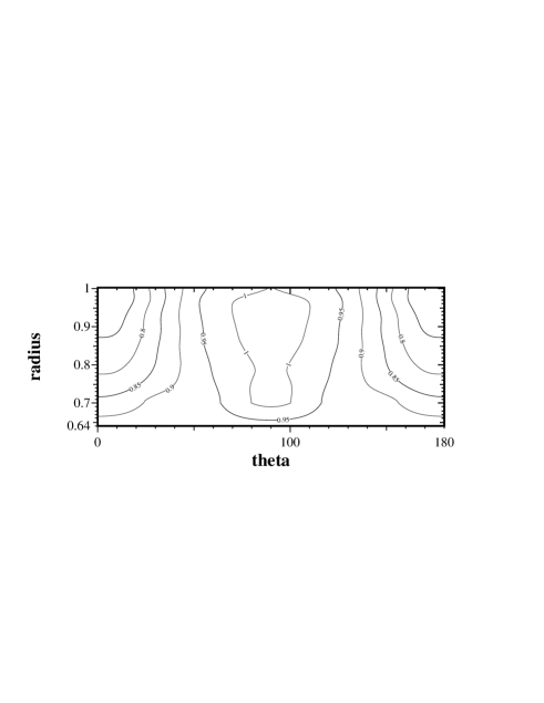
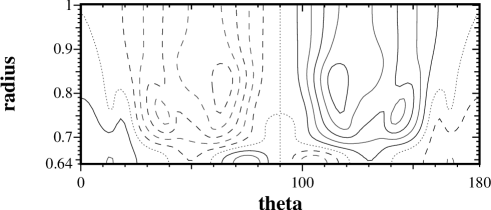
In the region we used an interpolation on the rotation law derived from helioseismic inversions. This was extended to include a tachocline region by interpolating between the helioseismic form at and solid body rotation at (see also Moss & Brooke 2000). Our choice gives a rather broad tachocline, but simplifies the numerics. Fig. 1 shows contours .
5 Results
5.1 Numerical implementation
We simulated the model described above in a meridional cross-section of a spherical shell with and .
The region was divided (rather arbitrarily) into 3 domains, namely , and and these were identified with the domains of the deep, middle and shallow active regions of Sect. 2. We attempt to identify the relative volume occupied by current helicity of ‘improper’ sign with .
5.2 A nonlinear solution
Our simulations show that the dynamo model leads to a steadily oscillating magnetic configuration for a quite substantial domain in the parameter space. These parameters seem acceptable when compared with current ideas in solar physics. We present here as a typical model with steady oscillations the case , (i.e. ), , , and . (With this value of , marginal excitation occurs when .) Of course, we are far from understanding helicity transport inside the Sun well enough to determine the numerical value of these parameters. The parameter set chosen gives a realistic time scale for the cycle period (about 10 years), but with a rather small nominal value of the turbulent diffusivity coefficient , i.e. this is how we choose to resolve the well-known problem with the length of solar cycle in the context of mean field dynamo models. The value (and ) chosen is perhaps larger then expected because we use the profile , which significantly reduces the mean value of over the domain compared to that with the ‘standard’ .
We demonstrated robustness with respect to the value of the parameter , which is associated with the magnetic Reynolds number: a uniform increase by two orders of magnitude makes quite small changes to our results, as does allowing a tenfold increase from top to bottom of the convection zone. When (i.e. smaller by a factor of 10 than in the basic run described above) we still obtain regular oscillations and the magnetic energy increases by a factor of 2 or 3 only. However, when is significantly smaller than 0.5, the solution becomes irregular. For we also verified that the differences between density parameter [Eq. (4)] (i.e. uniform density) and were small, and that allowing a radial dependence of also caused only small changes.
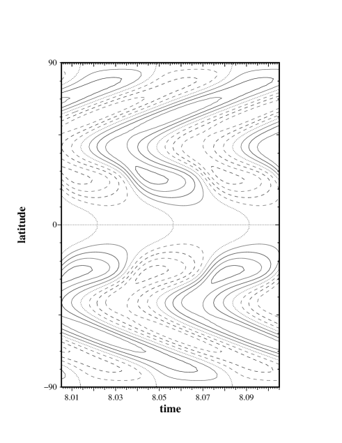
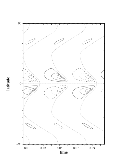
For this typical solution, the magnetic energy measured in the units of its equipartition value oscillates near the level , and the amplitude of the oscillations is about 0.035. This means that the averaged magnetic field strength is about 40% of the equipartition value. The magnetic configuration can be described as a system of activity waves which can be presented in the corresponding butterfly diagrams. In Fig. 2 we show the near-surface butterfly diagram (at ). Here, a pair of activity waves migrate from the middle latitudes towards the solar equator, while another pair migrates from the middle latitudes towards the poles. We present in Fig. 3 butterfly diagrams for the region just above the interface (at ). Here, both pairs of activity waves are much less pronounced in comparison to the structure shown in Fig. 2. However the equatorward branch now dominates the poleward. From these synthetic plots, it seems plausible that the observed butterfly diagram can be mimicked adequately. The magnetic field structure found in the simulations is also quite consistent with expectations.
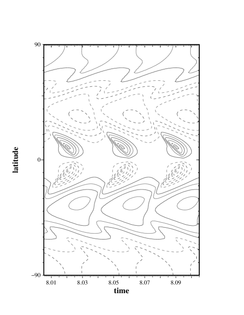
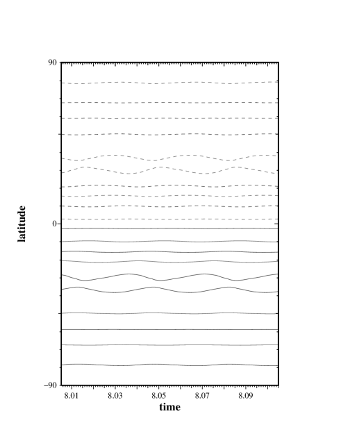

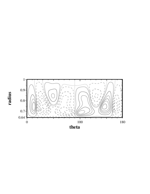
As a typical example, we give in Fig. 4 the toroidal magnetic field distribution for an instant soon after the minimum of magnetic energy. The current helicity distribution at the same time is given in Fig. 5. Here the dotted line indicates the zero contour of current helicity. The helicity distribution is antisymmetric with respect to the solar equator, but there are sign changes inside each hemisphere. If the helicity is basically positive in a given hemisphere (e.g. the southern), a region of negative helicity can be isolated near to the equator at the base of convective zone. The other region of opposite polarity in the helicity distribution is located near to the poles. Near the bottom of the convection zone, the helicity pattern migrates in a similar way to the toroidal field, and the corresponding butterfly diagram is given in Fig. 6. Quite unexpectedly, the helicity pattern near the surface does not demonstrate any pronounced migration (see Fig. 7).
Of course, we cannot claim a steady oscillating solution obtained for a rather arbitrary set of parameters should be directly confronted with proxies of solar activity (see Obridko & Shelting 2003). We note however that the solution obtained reproduces remarkably well some features of the solar cycle expected from dynamo theory and the observational data. Apart from a conventional equatorward migration, it demonstrates that the activity cycle is a complicated phenomenon which involves the Sun as a whole. We see an poleward migration at higher latitudes which is known from the polar faculae data (Makarov et al. 2001 and references therein, which give a modern viewpoint of the long-term research in this area) and from simple illustrative dynamo models (Kuzanyan & Sokoloff 1995, 1997). Such a pattern is also seen in the torsional oscillations, both as observed and as modelled by Covas, Moss & Tavakol (2004) – these are very plausibly intimately linked to the magnetic field variations. The magnetic field configuration looks quite simple and smooth for the surface butterfly diagram of toroidal magnetic field only. We see various magnetic field reversals inside the Sun. Such reversals have been suggested by many experts in solar activity whose analysis was not restricted to sunspot data (e.g. Benevolenskaya et al. 2002). The dynamo wave at the base of convective zone is much sharper and and localized (Fig. 3) than that nearer the surface (Fig. 2) – the latter appears closer to the current understanding of the solar cycle. Of course, it is at present unclear just what is the relation between the sites of field production by the dynamo and the manifestation of sunspots at the surface. The current helicity distribution is more complicated at the base of convective zone compared to that near the solar surface. This is in general agreement with the observational information concerning the radial distribution of solar helicity (Sect. 2).
The normalized local nonlinear dynamo number is shown in Fig. 8 at every point of the computational grid, as a function of mean magnetic field. Here is normalized by the local value of . The nonlinear dynamo number decreases with increase of the mean magnetic field. The latter dependence implies the saturation of the growth of the mean magnetic field in the nonlinear mean field dynamo. Note that the dynamo number which is based on the hydrodynamic part of the -effect increases with the mean magnetic field. This shows the very important role of the magnetic part of the -effect, which causes the saturation of the growth of the mean magnetic field.
5.3 The helicity distribution
We need to reduce the numerical data from our modelling to a form comparable with the observations available. The important point is that the resolution of the helicity observations is very substantially lower than that of the sunspot data, not to mention that of the dynamo simulations. The following procedure is applied to reduce the resolution of the numerical data, and so allow a meaningful comparison with the observations.
We isolate a region , i.e. a –belt centered on the equator, because helicity data are available for this equatorial domain only. We separate this region into a deep part, , and a shallow part with , and consider one hemisphere only, say the Northern (the simulated data are strictly antisymmetric with respect to the solar equator). Let and be the volumes inside each region where has a positive and negative sign respectively. We calculate the values and , where is the half length of the activity cycle (note that is negative).
From our basic run, we obtain the following values of the helicity integrals. For the ‘deep’ region (), we obtain and , while for the ‘shallow’ region we obtained and . The clear difference in helicity distribution between deep and shallow regions remains robust when the density parameter is reduced to [see Eq. (4)]. For the deep region (), we then obtain (of course, the equality is a pure coincidence) while for we obtained and .
We conclude that the available observational data concerning the radial distribution of current helicity seems to be consistent with the corresponding differences in numerical model. We consider the observed radial dependence of the current helicity as an observational manifestation of a structure similar to that presented in the numerical models.
Note that the choice of the latitudinal and radial belts in which the helicity integrals are calculated does affect significantly the numbers above. For our basic run, calculating the helicity integrals for the whole northern hemisphere we obtain and for , and for and , for . Obviously, these values of helicity integrals calculated for these more arbitrarily chosen belts are less impressive than the previous, where the belts were isolated on the basis of snapshots of the helicity distribution. The important thing is that a link between helicity integrals and depth is still visible here.
We stress that the available observational data, as well as the nature of the dynamo model, do not allow any quantitative description of the radial helicity distribution. The best that we can hope to do is to isolate some link between these quantities. The important result is that such a link appears to exist, without reference to a particular choice of boundaries. We stress this fact and do not take exactly the same boundaries in for shallow, middle and deep regions throughout the whole paper.
6 Discussion
In this paper we have demonstrated that the available observational data concerning solar current helicity give some hints concerning its radial distribution. The active regions clearly associated with the upper layers of solar convective zone demonstrate a significantly more homogeneous distribution of the current helicity than the deeper regions. We interpret this as an observational indication that the structure of the solar activity wave deep inside the Sun is substantially more complicated than near its surface. In contrast to a rather smooth structure of the surface activity wave with the dominant pattern propagating from the middle latitudes to the equator, we expect a more complicated structure of activity waves deep inside the Sun. In particular, the waves with ”wrong” polarity deep inside the Sun are expected to be more important compared to the main wave than nearer the surface.
We have demonstrated that the scenario of solar dynamo based on magnetic helicity conservation arguments can be extended to include radial dependence. This scenario leads to a steady oscillatory solution in a substantial domain of the parametric space, of a form that is at least consistent with our basic understanding of internal solar structure. If we choose a more extreme parameter set, it is natural that we will need to include more effects (say, buoyancy) into the dynamo saturation mechanisms.
Slightly unexpectedly, we note that the results of dynamo simulations are remarkably close to the available magnetic helicity observations. The structure of dynamo waves deep inside the convective zone is much sharper and more complicated than the smooth surface structure. The waves of ”wrong” polarity of helicity are pronounced in deeper layers and almost undetectable at the surface. We hope that this is an indication that our theoretical understanding of the solar dynamo has some observational support from helicity data. Of course, we stress that the very preliminary nature both of the topic and of our model prevents any strong conclusion, and that more observational and theoretical efforts are required to support our inferences. However, in any case the result obtained is perhaps as good as could be expected at the moment.
We emphasize that the ability of the observations to support (or reject) theoretical ideas concerning the radial properties of the solar activity wave is highly nontrivial. In contrast, we can neither support nor reject a scenario suggested by Choudhuri et al. (2004) who believe that the number of active regions violating the polarity law should be significantly larger at the beginning of the cycle rather in the later phases. Some tendency of this kind is visible in Tables 5 and 6, but the data are insufficient to support any firm statement. Further studies of a larger sample of active regions (cf. Bao et al. 2000, 2002) may help to address this point.
Note that the helicity distribution presented in Fig. 5 could be represented as a propagation of the activity wave from one hemisphere to the other. Suppose that a wave of negative helicity penetrates from northern hemisphere into the southern, where positive helicity dominates. Such a penetration of an activity wave into a ”wrong” hemisphere was investigated for Parker migratory dynamo by Galitski et al. (2005). They estimated the scale of penetration as about a dozen degrees in latitude, which seems broadly consistent with Fig. 5.
In our basic numerical model, the helicity close to the surface does not exhibit any migration. This perhaps seems quite unexpected, but does not directly contradict any observational or theoretical knowledge. Note that the butterfly diagrams for the mean surface poloidal magnetic field exhibit standing, rather than propagating, waves (Obridko & Shelting 2003).
Acknowledgments
We are indebted to Axel Brandenburg for illuminating discussions. The research was supported by grants 10233050, 10228307, 10311120115 and 10473016 of National Natural Science Foundation of China, and TG 2000078401 of National Basic Research Program of China. A very significant part of this work was performed during our (NK, DM, IR, DS) visit to the Isaac Newton Institute for Mathematical Sciences (University of Cambridge). DS and KK are grateful for support from the Chinese Academy of Sciences and NSFC towards their visits to Beijing. KK would like to acknowledge support from RFBR under grants 03-02-16384 and 05-02-16090. DS is grateful for financial support from INTAS under grant 03-51-5807 and RFBR under grant 04-02-16068. DM acknowledges support from the Royal Society during a visit to Moscow.
Appendix A Quenching functions
The quenching functions and appearing in the nonlinear effect are given by
| (10) | |||||
| (11) |
(see Rogachevskii & Kleeorin 2000), where
The nonlinear turbulent magnetic diffusion coefficients for the mean poloidal and toroidal magnetic fields, and , and the nonlinear drift velocities of poloidal and toroidal mean magnetic fields, and , are given in dimensionless form by
| (12) | |||||
| (13) | |||||
| (15) |
where
(Rogachevskii & Kleeorin 2004).
The functions are
The nonlinear quenching of the turbulent magnetic diffusion of the magnetic helicity is given by
| (16) |
References
- (1) Bao S. D., Ai G. X., Zhang H. Q., 2002, in Rickman H., ed., Highlights of Astronomy. Vol. 12, San Francisco, p. 392
- (2) Bao S. D., Ai G. X., Zhang H. Q., 2000, J. Astrophys. Astron., 21, 303
- (3) Bao S. D., Zhang H. Q., 1998, ApJ, 496, L43
- (4) Baker N., Temesvary S., 1966, Tables of Convective Stellar Envelope Models. New York
- (5) Benevolenskaya E. E., Kosovichev A. G., Lemen J. R., Scherrer P. H., Slater G. L., 2002, ApJL, 571, L181
- (6) Blackman E. G., Brandenburg A., 2002, ApJ., 579, 359
- (7) Brandenburg A., 2005, ApJ., 625, June 1
- (8) Brandenburg A., Subramanian K., 2004, Phys. Rept., submitted, and references therein. Also e-prints: astro-ph/0405052
- (9) Choudhuri A. R., Chatterjee P., Nandy D., 2004, ApJ., 615, L57
- (10) Collin B., Nesme-Ribes E., Leroy B., Meunier, N., Sokoloff D., 1995, Comptes Rendus, 321, II b, N 3, 111
- (11) Covas E., Tavakol R., Tworkowski A., Brandenburg A., 1998, A&A, 329, 350
- (12) Covas E., Moss D., Tavakol R., 2004, A&A, 416, 775
- (13) Galitski V. M., Sokoloff D. D., Kuzanyan K. M., 2005, Astron. Rep., 49, 337
- (14) Kleeorin N., Kuzanyan K., Moss D., Rogachevskii I., Sokoloff D., Zhang H., 2003, A&A, 409, 1097
- (15) Kleeorin N., Moss D., Rogachevskii I., Sokoloff D., 2000, A&A, 361, L5
- (16) Kleeorin N., Rogachevskii I., 1999, Phys. Rev. E, 59, 6724
- (17) Kleeorin N., Rogachevskii I., Ruzmaikin A., 1995, A&A, 297, 159
- (18) Kleeorin N., Ruzmaikin A., 1982, Magnetohydrodynamics, 18, 116. Translation from Magnitnaya Gidrodinamika, 2, 17 (1982)
- (19) Krause F., Rädler K.-H., 1980, Mean-Field Magnetohydrodynamics and Dynamo Theory. Pergamon, Oxford
- (20) Kuzanyan K. M., Lamburt V. G., Bao Sh. D., Zhang H., 2003, Chinese Journal of Astronomy and Astrophysics, 3, 257
- (21) Kuzanyan K. M., Sokoloff D., 1995, Geophys. Astrophys. Fluid Dyn., 81, 113
- (22) Kuzanyan K. M., Sokoloff D., 1997, Solar Phys., 173, 1
- (23) Longcope D. W., Fisher G. H., Pevtsov A. A., 1998, ApJ, 507, 417
- (24) Makarov V. I., Tlatov A. G., Sivaraman K. R., 2001, Solar Phys., 202, 11
- (25) Moffatt H. K., 1978, Magnetic Field Generation in Electrically Conducting Fluids. Cambridge University Press, New York
- (26) Moss D., Brooke J., 2000, MNRAS, 315, 521
- (27) Obridko V. N., Shelting B. D., 2003, Astron. Zh., 80, 364
- (28) Ossendrijver M., 2003, Astron. Astrophys. Rev., 11, 287
- (29) Parker E., 1955, ApJ, 122, 293
- (30) Pevtsov A. A., Canfield R. C., Metchalf T. R., 1994, ApJ, 425, L117
- (31) Pevtsov A. A., Canfield R. C., Metchalf T. R., 1995, ApJ, 440, L109
- (32) Pevtsov A. A., Canfield R. C., Latushko S. M., 2001, ApJ, 549, L261
- (33) Pouquet A., Frisch U., Leorat J., 1976, J. Fluid Mech., 77, 321
- (34) Rogachevskii I., Kleeorin N., 2000, Phys. Rev. E, 61, 5202
- (35) Rogachevskii I., Kleeorin N., 2004, Phys. Rev. E, 70, 046310
- (36) Rüdiger G., Brandenburg A., 1995, A&A, 296, 557
- (37) Seehafer N., 1990, Solar Phys., 125, 219
- (38) Schou J., Antia H. M., Basu S., Bogart R. S., Bush R. I., Chitre S. M., Christensen-Dalsgaard J., Di Mauro M. P., Dziembowski W. A., Eff-Darwich A., Gough D. O. , Haber D. A., Hoeksema J. T., Howe R., Korzennik S. G., Kosovichev A. G., Larsen R. M., Pijpers F. P., Scherrer P. H., Sekii T., Tarbell T. D., Title A. M., Thompson M. J., Toomre J., 1998, ApJ, 505, 390
- (39) Spiegel E. A., Weiss N. O., 1980, Nature, 287, 616
- (40) Spruit H. C., 1974, Solar Phys., 34, 277
- (41) Subramanian K., Brandenburg A., 2004, Phys. Rev. Lett., 93, 205001
- (42) Tobias S. M., Brummell N. H., Clune T. L., Toomre J., 2001, ApJ., 549, 1183
- (43) Tobias S. M., Hughes, D. W., 2004, ApJ., 603, 785
- (44) Vishniac E. T., Cho J., 2001, ApJ., 550, 752
- (45) Zhang H., Bao S., 1998, A&A, 339, 880
- (46) Zhang H., Bao S., 1999, ApJ., 519, 876
- (47) Zhang H., Bao S., Kuzanyan K. M., 2002, Astron Rep., 46, 414