Numeric simulation of relativistic stellar core collapse and the formation of Reissner-Nordstrom black holes

Abstract

The time evolution of a set of $22M_{\odot}$ unstable charged stars that collapse is computed integrating the Einstein-Maxwell equations. The model simulate the collapse of an spherical star that had exhausted its nuclear fuel and have or acquires a net electric charge in its core while collapsing. When the charge to mass ratio is $Q/\sqrt{G}M\geq 1$ the star do not collapse and spreads. On the other hand, it is observed a different physical behavior with a charge to mass ratio $1>Q/\sqrt{G}M>0.1$. In this case, the collapsing matter forms a bubble enclosing a lower density core. We discuss an immediate astrophysical consequence of these results that is a more efficient neutrino trapping during the stellar collapse and an alternative mechanism for powerful supernova explosions. The outer space-time of the star is the Reissner-Nordström solution that match smoothly with our interior numerical solution, thus the collapsing models forms Reissner-Nordström black holes.

I INTRODUCTION

In this work we intend to study the effects of an electric field on the collapse of a massive star. We perform direct relativistic simulations assuming spherical symmetry and integrating the Einstein-Maxwell equations. We studied the collapse of several stars with different values of the total electric charge and determined the limits at which the collapse is avoided by the effect of the repulsive electric field. The electric charge is carried by the particles that compose the collapsing fluid. The electromagnetic field and the internal energy of the gas contributes to the total mass-energy of the star, so it is not clear whether it is possible to overcharge a collapsing configuration. The analysis and conclusions drawn for collapsing charged shells cannot be directly extrapolated for this case, and a complete relativistic calculation performed in a self-consistent way is needed to know the outcome of the charged collapse.

In particular, we found the formation of a bubble that was not predicted before. Although its theoretical explanation is quite natural, the formation of the bubble depends on the initial conditions and its evolution is far from obvious due to the non-linearities of the Einstein-Maxwell equations. Numerical solutions for the problem of charged stellar collapse were found only recently ghezzi2 , .

It is commonly assumed that the stars are nearly neutrally charged due to a mechanism of selective accretion of charges from the surrounding interstellar medium. Therefore, if a star is initially positively (negatively) charged, accretion of negative (positive) charges from the surrounding gas will tend to neutralize the total net charge. The same reasoning is applied to black holes wald . We observe that the effect of selective accretion were never fully calculated to our knowledge. On the other hand, an star can be electrically neutral while possessing a huge internal electric field .

The internal electric field of an astronomical object can be very large in some special scenarios zeldovich , olson1 , olson2 , shvartsman . In particular, the charge separation inside a spherical compact star, in hydrostatic equilibrium, can be very large when one of the plasma components is a degenerate gas while the other is a Maxwell-Boltzmann gas, i.e., like the gas of degenerated electrons and the gas of nuclei in a white dwarf olson2 .

The calculations presented in this paper corresponds to the case in which the star posses a net electric charge. However the results can be taken as an approximation to the more complicated problem of an star with total zero charge and with a non zero internal electric field. We leave this point aside and for clarity we will concentrate here on the dynamics of an star with a total positive charge.

We ask whether an electrically charged star can collapse to form a charged black hole. Would the Coulomb repulsion avoid the collapse of the star ?, and moreover, are there physical differences with the physics of uncharged collapse ?. Moreover, from pure analytic analysis is not clear if it is possible to form an overcharged black hole (with $Q>\sqrt{G}M$). The dynamics of a collapsing star could be quite different from the collapse of a charged shell onto an already formed Reissner-Nordström black hole, mainly due to backreaction effects. In the present paper, we will try to give the answer to these questions.

Extremely charged black holes ($Q/\sqrt{G}M=1$) represent an extreme limit in the context of the cosmic censorship hypothesis, since bodies with charge equal or higher than extremal are undressed by event horizons and constitutes naked singularities joshi , wald . On the other hand, the formation of Reissner-Nordström (RN) black holes, is in connection with the third law of black hole thermodynamics anninos , israel , ghezzi2 , because an extreme RN black hole has zero temperature. So, there is an interest on the formation of charged black holes from a pure theoretical point of view .

In this paper we are not concerned with the mechanism that produce charge or an internal electric field. Neither magnetic fields nor rotation are taken into account, although they could increase the magnitude of the electric fields.

Without loss of generality, the density of charge was chosen proportional to the rest mass density. The interior solutions found can be matched smoothly with the Reissner-Nordström exact solution for the vacuum space-time ghezzi2 . Therefore, in the cases in which the star collapses the result is the formation of a Reissner-Nordström black hole.

The paper is organized as follows. In Section II, we discuss the problem of charged collapse analyzing the order of magnitude of the physical quantities. In the Section III are described the general relativistic equations that govern the dynamics of the stellar core collapse. In Section IV, are described the numerical techniques used to integrate the general relativistic equations and some caveats on its applications. Section V brings a discussion and interpretation of the numerical results. In the Subsection A, we show the calculation of the maximum mass formula for Newtonian charged stars, and in Subsection B we calculate the optical depth for the neutrinos emitted during the collapse. We also discuss the implications for core collapse supernova. We end in Section VI presenting some final remarks.

II Some order of magnitude estimates

In this section we show some order of magnitude estimates, in order to put in a clear perspective the problem of a self-gravitating charged fluid sphere. The calculations in the present section are valid only in the non-relativistic regime.

The formation of a charged star, is possible when the gravitational attraction overwhelms the electrostatic repulsion on each single particle of the gas that is collapsing, i.e.,

$$F_{grav}\geq F_{elect}\,,$$ (1)

or equivalently

$$q\,Q_{s}\geq m\,M_{s}\,,$$ (2)

where $Q_{s}$ and $M_{s}$ are the charge and mass of the star and $q$ and $m$ are the charge and mass of the particles. In this section we use a Newtonian approach, the full relativistic case could be different.

Assume a star that has a total charge to mass ratio $Q_{s}/\sqrt{G}M_{s}$. According to Eq. (2) any particle with a charge to mass ratio $q/\sqrt{G}m$ can be added to the star if

$$\alpha_{1}\equiv\frac{Q_{s}}{\sqrt{G}\,M_{s}}\leq\biggl{(}\frac{q}{\sqrt{G}\,m}\biggr{)}^{-1}\,,$$ (3)

where the equality gives the maximal charge to mass ratio

$$\alpha_{1}=\biggr{(}\frac{q}{\sqrt{G}\,m}\biggl{)}^{-1}\,.$$ (4)

For example, a proton has a charge to mass ratio $q_{p}/\sqrt{G}m_{p}\sim 10^{18}$. Using the Eq. (3) the proton can be added to the charged star if

$$\frac{Q_{s}}{\sqrt{G}\,M_{s}}\leq 10^{-18}\,.$$ (5)

Thus, a star with higher charge to mass ratio can not be assembled from protons alone. On the other hand, if the infalling particles are dust particles with a larger charge to mass ratio, the maximum limit for the charge to mass ratio of the charged star can be much higher.

An example of this is a self-gravitating ball of FeI nucleus, of mass $M_{ball}$ and charge $Q_{ball}$. As the charge to mass ratio for FeI is $q/\sqrt{G}m\sim 10^{16}$, the Eq. (3) for Fe gives

$$\alpha_{2}=\frac{Q_{ball}}{\sqrt{G}\,M_{ball}}\leq 10^{-16}\,,$$ (6)

and we see that in this case $\alpha_{2}\gg\alpha_{1}$ (greater than for protons alone, see Eq. (5) above).

For “charged dust” formed by particles with $q/\sqrt{G}m\sim 1$, a self-gravitating sphere with mass $M_{dust}$ and charge $Q_{dust}$, can be in hydrostatic equilibrium if:

$$\alpha_{3}=\frac{Q_{dust}}{\sqrt{G}\,M_{dust}}\sim 1\,.$$ (7)

So : $\alpha_{3}\gg\alpha_{2}\gg\alpha_{1}$. Let us estimate the amount of charge needed to have an extremely charged $10\,M_{\odot}$ star. In this case $Q_{star}/\sqrt{G}\,M_{star}=1$, so

$$Q_{star} =\sqrt{6.67\,\,10^{-8}}\times 10\times 1.9\,\,10^{33}$$ (8)

$$=4.9\times 10^{30}\,\,{\rm statCoulomb}\,.$$

Therefore, it is needed to have an excess of

$$\sim Q_{star}/q_{p}=10^{40}\,\,\,\,\,\,{\rm charges}\,,$$

in the star, where $q_{p}=4.803\times 10^{-10}\,\,{\rm statCoulomb}$ is the charge of one proton. There is roughly $\sim 10^{58}$ baryons in a $10M_{\odot}$ star. So, there must be one charged particle on $\sim 10^{18}$ neutral ones in order to have a maximally charged compact object. This is compatible with the limits given above. Therefore, in the extremal case, there are a small charge imbalance equal to:

$$\delta Q\sim 10^{-18}\,\,\,\,{\rm charges\,\,per\,\,baryon}\,,$$ (9)

in the star. A tiny amount of charge from a microscopic point of view, but with a huge total sum (see Ref. ghezzi2 ).

It is possible to make the objection that the nucleus would disintegrate, or suffer nuclear fission, before assembling a charged star. However the energy locally available (in the center of mass of the particles) from the collapse is not enough to unbind a nucleus (bounded by the strong force). This was calculated for a compact charged neutron star. An exception is a nearly extremal compact object, in this case is energetically favorable for the nucleus to disintegrate ghezzi2 . The conclusion is that we can approach to the formation of a “nearly extreme” object, although it is not possible to reach the extremal value, the particles will fission first (see ghezzi2 for details).

Studying theories with extra dimensions, Mosquera-Cuesta and co-workers mosquera found that particles located in the brane can leak out to the bulk space. It results that electrons can leak out more easily than baryons, producing a charge asymmetry that can be very large in very old stellar systems. This is suitable for type II supernova progenitors and neutron stars ghezzi2 . The mechanism produce a charge imbalance of mosquera :

$$\delta Q\sim 10^{-14}-10^{-16}\,\,\,\,{\rm charges\,\,per\,\,baryon}\,.$$ (10)

This is several orders of magnitude higher than the needs for producing an extremal star. Therefore, charged old stars must be considered and studied as a theoretical possibility.

III Equations in co-moving coordinates

We want to solve the Einstein-Maxwell equations (see Ref. ghezzi2 ):

$$R^{\mu\nu}-\frac{1}{2}g^{\mu\nu}R=\frac{8\pi G}{c^{4}}T^{\mu\nu}\,,$$ (11)

where $R^{\mu\nu}$ is the Ricci tensor, $g^{\mu\nu}$ is the metric tensor, $R$ is the scalar curvature, and $T^{\mu\nu}$ is the energy momentum-tensor, composed by two parts:

$$T^{\mu\nu}=T_{F}^{\mu\nu}+T_{M}^{\mu\nu}\,$$ (12)

the perfect fluid energy-momentum tensor $T_{F}^{\mu\nu}$ and the Maxwell energy-momentum tensor $T_{M}^{\mu\nu}$. The electromagnetic energy-momentum tensor is given by:

$$T_{M}^{\mu\nu}=\frac{1}{4\pi}\biggl{(}F^{\mu\alpha}F^{\nu}_{\,\,\,\alpha}-\frac{1}{4}g^{\mu\nu}F_{\alpha\beta}F^{\alpha\beta}\biggr{)}\,,$$ (13)

here $F^{\mu\nu}$ is the Maxwell electromagnetic tensor, which can be written in terms of a potential $A^{\mu}$:

$$F_{\mu\nu}=A_{\mu;\nu}-A_{\nu;\mu}\,.$$ (14)

In the last equation and in the rest of the paper, we use semi-colon to denote covariant derivative. The perfect fluid energy-momentum tensor is:

$$T_{F}^{\mu\nu}=(P+\delta\,c^{2})\,u^{\mu}u^{\nu}-P\,g^{\mu\nu}\,,$$ (15)

where $\delta\,c^{2}$ is the density of mass-energy and $P$ is the pressure, given in ${\rm[dyn/cm^{2}]}$, and $u^{\nu}$ is the $4$-velocity of the observers co-moving with the fluid landau , weinberg , ghezzi2 . The electromagnetic tensor must satisfy the Maxwell equations bekenstein , mashhoon , ghezzi2 :

$$F^{\mu\nu}_{\,\,\,\,\,;\nu}=4\pi j^{\mu}\,.$$ (16)

From Eq. (14) and using the Bianchi identities, we have:

$$F_{[\alpha\beta;\gamma]}=0\,.$$ (17)

We will use the common split of the energy:

$$\delta=\rho\,(1+\epsilon/c^{2})\,,$$ (18)

where $\rho$ is the rest mass density, and $\rho\,\epsilon$ is the internal energy density ghezzi2 , shapiro .

The fluid must satisfy the energy-momentum conservation equation:

$$T^{\mu\nu}_{\,\,\,\,\,\,;\nu}=0\,,$$ (19)

and the baryon conservation equation:

$$(\rho\,u^{\nu})_{;\nu}=0\,.$$ (20)

We will write the Einstein-Maxwell equations in coordinates and gauge choice appropriated for its numeric implementation ghezzi2 . Considering a spherical star, the line-element in co-moving coordinates is given by

$$ds^{2}=a(t,\mu)^{2}c^{2}dt^{2}-b(t,\mu)^{2}d\mu^{2}-R(t,\mu)^{2}d\Omega^{2}\,.$$ (21)

The 4-velocity of an observer co-moving with the fluid is $u^{\nu}=[a^{-1},0,0,0]\,,$ and satisfies $u^{\nu}u_{\nu}=c^{2}$, where $c$ is the speed of light. The coordinate $\mu$ was gauged to be the rest mass enclosed by co-moving observers standing on spherical layers of the star. Each layer has its own constant value of $\mu$. In particular, observers at the surface of the star will be designated with a coordinate $\mu=\mu_{s}$.

We define

$$u=R_{,t}/a\,.$$

So, the equation of motion, obtained from the Einstein-Maxwell equations ghezzi2 is

$$u_{,t}=-a\,\biggl{[}4\,\pi\,R^{2}\,\frac{\Gamma}{w}\,\biggl{(}P_{,\mu}-\frac{Q\,Q_{,\mu}}{4\,\pi\,R^{4}}\biggr{)}+\frac{G\,m}{R^{2}}+$$

$$\frac{4\,\pi\,G}{c^{2}}\,P\,R-\frac{G\,Q^{2}}{c^{2}\,R^{3}}\biggr{]}\,,$$ (22)

where $w=1+\epsilon/c^{2}+P/\rho c^{2}$ is the relativistic specific enthalpy, $\rho$ is the rest mass density, $\epsilon$ is the internal energy per unit mass, $P$ is the pressure, $G$ is the gravitational constant, $Q(\mu)$ is the total charge integrated from the origin of coordinates up to the spherical layer with coordinate $\mu$, and $m=m(t,\mu)$ is the total mass-energy defined below. We use the notation $f_{,x}=\partial f/\partial x$, with $x=\{\mu,t\}$, throughout the paper.

We note that the Eq. (III) resembles a Newtonian equation of motion plus relativistic corrections. In the Eq. (III) the last two terms are pure relativistic, and the full equation is equivalent to its Newtonian counterpart when $c\rightarrow\infty$ . The factor $\Gamma$ is a generalization of the special-relativistic $\gamma$ factor for general relativity and is given by

$$\Gamma^{2}=1+\frac{u^{2}}{c^{2}}-\frac{2\,m\,G}{R\,c^{2}}+\frac{G\,Q^{2}}{c^{4}\,R^{2}}\,.$$ (23)

This factor also verifies the equality $\Gamma=R_{,\mu}/b$ (see Refs. ghezzi2 , may , bekenstein ).

The equation for the metric component $a=g_{tt}^{1/2}/c$ is obtained from the energy-momentum conservation equation $T_{1;\nu}^{\nu}=0$, and is given by ghezzi2

$$\frac{(aw)_{,\mu}}{aw}=\frac{1}{wc^{2}}\biggl{[}\epsilon_{,\mu}+P\,\biggl{(}\frac{1}{\rho}\biggr{)}_{,\mu}+\frac{Q\,Q_{,\mu}}{4\,\pi\,R^{4}\rho}\biggr{]}\,.$$ (24)

The other independent component $T_{0;\nu}^{\nu}=0$ gives

$$\epsilon_{,t}=-P\,\biggl{(}\frac{1}{\rho}\biggr{)}_{,t}\,,$$ (25)

which is identical to the non-relativistic adiabatic energy conservation equation, and constitutes the first law of thermodynamics. We observe that the Eq. (25) do not contain any electromagnetic term. This is due to the symmetry of the problem, although an electromagnetic term arise in the total energy (see the Eq. 28 below).

From the conservation of the number of baryons, we obtain the equation for the metric component $b=g_{\mu\mu}^{1/2}$ ghezzi2 ,

$$b(t,\mu)=\frac{1}{4\,\pi\,R^{2}\,\rho}\,.$$ (26)

The Lagrangian coordinate $\mu$ can be chosen to be ghezzi2

$$\mu=4\,\pi\,\int_{0}^{R^{\prime}}\rho\,R^{2}dR/\Gamma\,,$$ (27)

this is the total rest mass enclosed by a sphere of circumference $2\,\pi\,R^{\prime}$. Thus, the collapsing ball is divided in layers of constant rest mass $\mu$ and each co-moving observer is at rest in each of this layers .

The equations for the total mass and the mass conservation are, respectively ghezzi2 :

$$m(t,\mu)=4\,\pi\,\int^{\mu}_{0}\rho\,\biggl{(}1+\frac{\epsilon}{c^{2}}\biggr{)}\,R^{2}\,R_{,\mu}\,d\mu\,\,+$$ (28)

$$\frac{1}{c^{2}}\int^{\mu}_{0}\frac{Q\,Q_{,\mu}}{R}\,d\mu\,;$$

$$(\rho R^{2})_{,t}/\rho R^{2}=-a\,u_{,\mu}/R_{,\mu}\,.$$ (29)

The charge 4-current $j^{\nu}$ is the product of a scalar electric charge density $\rho_{ch}$ times $u^{\nu}$ ; $j^{\nu}=\rho_{ch}\,u^{\nu}$. It can be shown that the charge and the rest mass are conserved in shells co-moving with the fluid bekenstein , ghezzi2 . So, the charge increment between layers can be written as being proportional to $d\mu$,

$$dQ=4\,\pi\,\rho_{ch}\,R^{2}\,dR/\Gamma\,,$$ (30)

where $\rho_{ch}\propto\rho$.

We observe that Eq. (30) is a non-linear equation, since $\Gamma$ depends on the integral value of the charge $Q(\mu)$ (see Eq. 23), so the set of equations above must be solved self-consistently.

The equations (III)-(30) above are solved numerically with the following boundary conditions:

$$P=0,\,\,\,{\rm at}\,\,\mu=\mu_{s},\,\,\,\,\forall\,t\,,$$ (31a)

$$a=1,\,\,\,\,{\rm at}\,\,\mu=\mu_{s},\,\,\,\,\forall\,t\,,$$ (31b)

$$u=0,\,\,\,\,{\rm at}\,\,t=t_{0},\,\,\,\forall\,\mu\,,$$ (31c)

$$R=0,\,\,\,{\rm at}\,\,\,\mu=0,\,\,\,\forall\,t\,,$$ (31d)

where $\mu_{s}$ is the mass coordinate at the surface of the star. The boundary condition (31a) can be derived from the matching condition between the interior and the exterior solution ghezzi2 . Equation (31b) express our coordinate freedom to choose the time synchronized with a co-moving observer moving with the surface of the star. Eq. (31c) means that the ball is initially at rest (at the initial time $t_{0}$), and Eq. (31d) is the impenetrability condition at the origin of coordinates (this condition can be stated equivalently as $u=0$ at $\mu=0$). In the next section we will present the initial conditions.

In this work we choose

$$\rho_{ch}=constant\,\times\,\rho\,,$$ (32)

for simplicity and without loss of generality.

IV Numerical techniques and code setup

The equations given in the section above are written in a form closely paralleling the equations of May and White ghezzi , ghezzi2 , for the non-charged case may , may2 , voropinov .

We built the numerical code collapse05v2 to integrate the Eqs. (III)-(30).

The Eq. (24) is re-written as ghezzi2 :

$${aw} = {a_{0}w_{0}}\,{\rm exp}\,\biggl{[}\,\int_{0}^{\mu_{s}}\,\biggl{(}d\epsilon+P\,d\biggl{(}\frac{1}{\rho}\biggr{)}+$$ (33)

$$\frac{Q\,dQ}{4\,\pi\,r^{4}\,\rho}\biggr{)}/w\,c^{2}\biggr{]}\,.$$

This equation is integrated numerically from the surface of the star toward the center, using the boundary condition $a_{s}\,w_{s}=1$, where $a_{s}$ and $w_{s}$ are given at the surface of the star (with coordinate $\mu_{s}$), note that we already choose $a_{s}=1$ (see Eq. 31b).

The collapse05v2 uses a leapfrog method plus a predictor corrector step, and iterates with a Crank-Nicholson algorithm. The method is second order accurate in time and space. We use a numerical viscosity to resolve the strong shock waves formed may2 .

IV.1 Initial conditions and numerical caveats

It is assumed a charge density proportional to the rest mass density through the star: $\rho_{ch}/\sqrt{G}\rho\sim constant$. From Eqs. (27) and (30) we see that $Q(\mu)/\sqrt{G}\mu=constant$, $\forall\,(t,\mu)$.

We assumed a polytropic equation of state, $P=k\rho^{\gamma}$, where $\gamma=5/3$ is the adiabatic coefficient . The star has initially a uniform mass density, $\rho=10^{7}\,{\rm g\,\,cm}^{-3}$ and a uniform distribution of electric charge density, in all the models studied. The initial specific internal energy $\epsilon$ is varied in the different simulations. The initial setup imitates a massive star of $M=21.035M_{\odot}$ that had exhausted its nuclear fuel. Its fate depends on the internal energy and charge of the initial configuration. This is explored with our simulations. The initial radius of the star is $R_{0}=10^{9}$ cm, in all the simulations.

Also we consider that the electric field is always much lower than the Schwinger field limit for pair creation ($\sim 10^{16}$ Volt/cm, in vacuo and in flat space-time Schwinger ). For example, in the case of extremal charge $Q/\sqrt{G}M=1$, the total charge will be $Q\sim 10^{31}$ stat-Coulomb. In this case, the maximum electric field strength is $\sim 10^{11}$ stat-Volt/cm or $\sim 3\times 10^{15}$ Volt/cm. However, during the collapse the field can strengthen and take higher values, so quantum effects would be taken into account in a more realistic approach.

We are not considering magnetic fields in the present simulations .

The simulations converge to the same solution when the resolution or the viscosity parameter are changed. The parameters of the simulation were chosen for accuracy and efficiency when running on a single processor. We performed the simulations using an Intel Pentium IV 2.6 Ghz processor (32 bits) and compiled the code with Lahey/Fujitsu v6.1 lahey for 32 bits; also we used an AMD Athlon FX 2.6 Ghz processor (64 bits) and compiled with Absoft absoft for 64 bits, running under Linux operating system. The code also runs under the Windows operating system and compile with the Fortran 90 Power Station. We didn’t find essential differences between the different runs with the exception of the speed of the simulation, which is faster with the AMD processor. In addition we set: a) the number of integration points: 1000; b) viscosity parameter: $3.3$; c) initial time-step: $10^{-5}\,$sec. We also performed tests simulations with 300 and 1500 points to be sure of the physical results, and tested the code varying the viscosity over a wide range of parameters. In the present simulations we tried to minimized the effects of the viscosity while keeping the ability of the code to resolve shock fronts.

The percentage of numerical error in the Hamiltonian constraint, expressed by the conservation of the total mass-energy $m(t,\mu_{s})$, is given by:

$$E_{H}=100\,\times\,|m-m^{\prime}|/m\,,$$

where $m^{\prime}=m^{\prime}(\mu_{s})$ is the exact value of the total mass energy (constant in time) and $m=m(t,\mu_{s})$ is the numerical value. The momentum constraint is “build in” the code and exactly conserved. In the present simulations: $E_{H}<0.1\,\%$ when the AH forms, using $1000$ points, and it is $E_{H}<0.009\,\%$ with $1500$ points, with no essential qualitative differences between the solutions. This values of $E_{H}$ are for the worst case of a large binding energy and with very strong shocks, so it can be considered as the superior bound of the error.

After crossing the AH the error grows to: $\sim 0.4\,\%$ (using $1000$ points), and the simulation is stopped. Thus in every simulation we set a maximum error tolerance of $E_{H}\sim 0.4\,\%$. We checked that using a higher number of points the errors are reduced.

We emphasize that the numerical errors (mainly $E_{H}$, not the roundoff errors) and the intrinsic difficulty on the simulation is the formation of the black hole region, because near it several numerical operators blows up.

IV.2 The apparent horizon

For each layer of matter with Lagrangian coordinate $\mu$ it is possible to define an internal and an external horizon,

$$r_{\pm}(t,\mu)=\frac{Gm(t,\mu)}{c^{2}}\pm\frac{G}{c^{2}}\sqrt{m^{2}(t,\mu)-Q^{2}(\mu)/G}\,,$$ (34)

which can be interpreted as a generalization of the Schwarzschild radius for charged stars. During the simulation an apparent horizon forms when some layer of matter cross its external horizon, i.e. when: $r(t,\mu)\leq r_{+}(t,\mu)$ ghezzi2 . In addition to the formation of the apparent horizon, in some cases a coordinate singularity develops, i.e.: $g_{tt}(t,\mu^{\prime})\rightarrow 0$ and $g_{\mu\mu}(t,\mu^{\prime})\rightarrow+\infty$ (for some coordinate value $\mu^{\prime}\neq 0$). Note that at the coordinate $\mu=0$ is located the physical timelike singularity of the vacuum Reissner-Nordström space-time. The simulation must be ended before any observer $\mu$ can meet its internal horizon $r_{-}(\mu)$. Hence, we can not say if the star collapses directly to a singularity or if it pass through a wormhole to another asymptotically flat universe. In this paper, we leave this question open.

The formation of an apparent horizon (AH) is a sufficient condition (although not necessary) for the formation of an event horizon and a black hole region ghezzi2 . Moreover, the interior solution matches with the exterior Reissner-Nordström spacetime ghezzi2 . In this sense, we can say that the outcome of the simulations in which an AH forms is the formation of a “Reissner-Nordström black hole”. Of course, if not all the matter collapse to the AH the result at the moment the simulation is stopped will be an electric black hole plus a surrounding gas with a vacuum Reissner-Nordström exterior spacetime.

We observe that there must exist other formulations of the problem in which it is possible to get closer to the singularity while avoiding the AH. We will explore this subject in future works.

V Discussions of the results

We performed a set of simulations on the collapse of a $21\,M_{\odot}$ star varying the initial conditions. We found that for certain cases a shell-like structure of higher mass density and charge is formed in the most external part of the star. This shell enlarge with time until it reaches the center of the star.

The Table I summarize the results of the simulations performed. In each model studied are different amounts of total electric charge; initial internal energy or binding energy. The fate of each model depends on this conditions.

The formation of the shell is sensible to the internal energy, or the binding energy, of the star (see Table I). When stronger is the bound of the star higher is the wall of the shell.

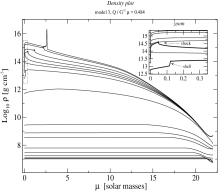
Figure 1: Snapshots of the mass density versus the mass coordinate $\mu$, for the model 3 of the Table I, the shell forms mildly in this case, although the shock is very strong.

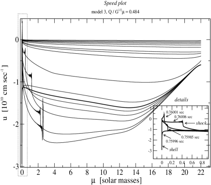
Figure 2: Snapshots of the speed versus the Lagrangian mass, the inset shows the details of the shell impinging on the center and the shock starting its propagation. The speed is positive during a short lapse of time.

In the Fig. (1), we show the profiles of the mass density versus the Lagrangian mass $\mu$ for the model $3$ of the Table I, in this case the shell forms only mildly. However, there is a strong shock wave formed. The Fig. (2) shows the velocity profiles, on which it is seen a strong shock propagating outwards. We observe that although the shock is propagating outwards the sign of the fluid velocity is negative everywhere indicating that the star is always collapsing. There is an exception in which the shock velocity acquires a positive sign, although it lasts a very brief period of time. This is shown on the inset of the Fig. (2): the shell is reaching the coordinate origin, and an instant later it impinges the center. After that a shock wave is formed and start to propagate outwards. During a brief lapse of time the velocity is positive, although the shock is not strong enough to stop the total collapse. The Figure (3) contains the snapshots of the metric component $g_{tt}^{1/2}$: it can be seen that concordant with the shell impinging the center, $g_{tt}$ acquires a value greater than one, indicating a blueshift with respect to the infalling matter. The inset of the Fig. (3) shows the details of the jumps produced on the value of $g_{tt}^{1/2}$ at the shell and at the shock positions, as well as the mentioned blueshift.

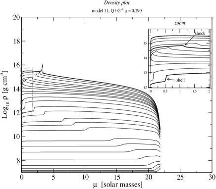
Figure 4: Snapshots of the mass density versus $\mu$, for the model 11 of the Table I. In this case there is an important imploding shell. The dotted box is zoomed on the inset, which shows the shell impinging at the center and the shock forming and propagating outwards.

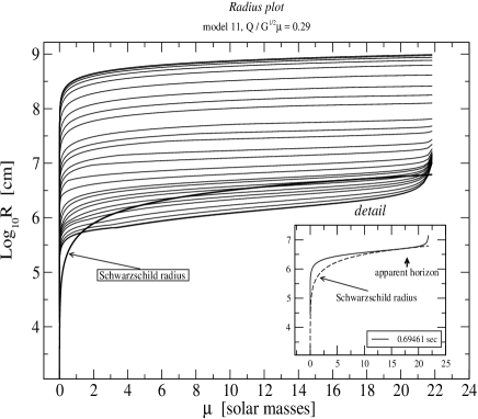
Figure 5: The radius (Log₁₀Radius) versus the Lagrangian mass, the bold line shows the Schwarzschild radius at the instant of the apparent horizon formation, the inset box shows the detail of an observer crossing his/her own Schwarzschild radius (an arrow is pointing the observer) and signaling the formation of an apparent horizon. It can be appreciated that the simulation continues far beyond the formation of the apparent horizon.

Figure (4) contains the snapshots of the mass density for the model $11$ of the Table I. In this case there is an strong shell formed. On this figure we can see that the shell propagates inwards, to lower values of the Lagrangian coordinate $\mu$, until it impinges the center. At this moment, and place, it is formed an strong shock that starts its outward propagation. The inset box of the Figure (4) is a zoom of the dotted box, showing the details of the collapsing shell and the shock formed. The Fig. (5) shows the verification that the collapse produce a black hole. In spherical symmetry the apparent horizon is formed simply when an observer cross his/her own Schwarzschild radius. The inset box of the Fig. (5) shows the radius profile at the moment that the curve touch the Schwarzschild radius profile at a point. That point indicates an observer crossing the Schwarzchild radius and is the locus of the apparent horizon. After then the apparent horizon will evolve approaching the event horizon at infinite coordinate time or after complete collapse (not calculated).

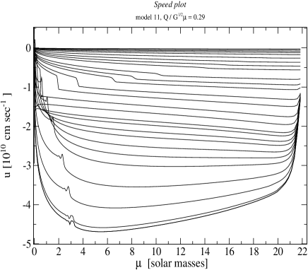
Figure 6: Snapshots of the speed versus $\mu$ for model 11, it can be observed a jump in the velocity profile at the shell position dislocating through the center of the star. See Fig. (7).

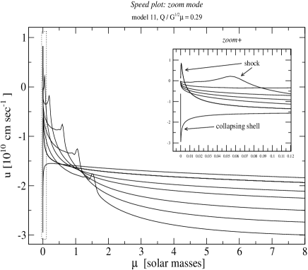
Figure 7: Detail of the speed’s profile showing the moment of time the shell impinges at the center of the star, later the shock is formed and starts its outward propagation, the inset shows a zoom of the dotted box. See Fig. (6).

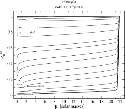
Figure 8: Temporal snapshots for $\sqrt{g_{tt}}$ versus $\mu$ for model 11 and its late collapse to zero. We must observe that the apparent horizon forms before $g_{tt}\rightarrow 0$, which indicates the convergence towards the event horizon.

Figure (6), shows the velocity profiles for model 11, there is an strong-shell and strong-shock in this case. However, the velocity has a negative sign and the matter collapse directly to a black hole. Figure (7) shows the speed profile at the moment of time in which the shell impinges the center, and the formation and propagation of the shock wave. The inset box shows a close up of the details. There is a short lapse of time in which the shock has positive velocity. The Fig. (8) shows the metric coefficient $g_{tt}^{1/2}$ going to zero. In this case $g_{tt}$ never becomes greater than one, and the inner matter is always redshifted respect to observers standing at the surface or outside the star.

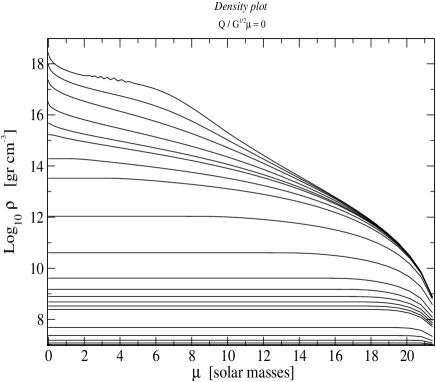
Figure 9: Snapshots of the mass density versus $\mu$ for model 13, an uncharged star.

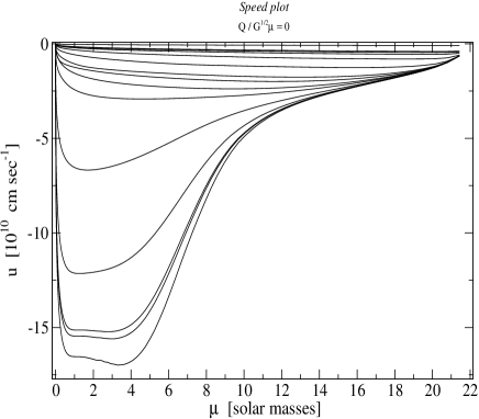
Figure 10: Snapshots of the speed profile, where $u$ has the meaning of the rate of radius change per unit proper (comovel) time change.

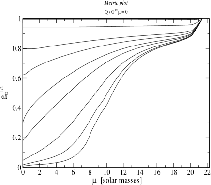
Figure 11: Temporal snapshots for $\sqrt{g_{tt}}$ versus $\mu$ for model 13.

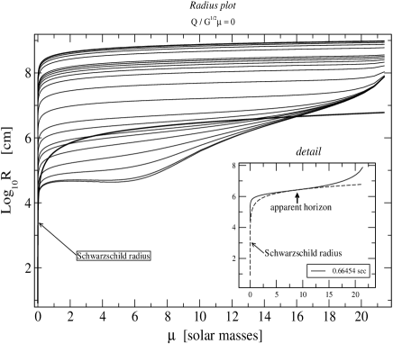
Figure 12: The radius versus $\mu$: the bold line shows the Schwarzschild radius at the instant of time the apparent horizon is formed, the inset shows the detail of an observer, pointed with an arrow, crossing his/her own Schwarzschild radius, indicating the formation of an apparent horizon at this coordinate and at the time indicated.

Figure (9) shows the density snapshots for the collapse of an uncharged star (model $13$). It is possible to compare this simulation with the former simulations, we see that for the charged collapse the density profiles are flatter all the way through the black hole formation. Figure (10) shows the velocity profiles (compare it with the Figs. 2 and 6). The Figure (11) shows the collapse of $g_{tt}^{1/2}$ (compare it with the Figs. 3 and 8). Figure (12) shows the profiles of the metric function $R$, the bold line is the Schwarzschild radius at the moment the apparent horizon forms. The inset box shows the detail of the radius profile touching the Schwarzschild profile at one point, signaling the formation of an apparent horizon at the point indicated with the vertical arrow, at the time indicated on the legend box. The simulation is continued beyond that event, as seen in this figure.

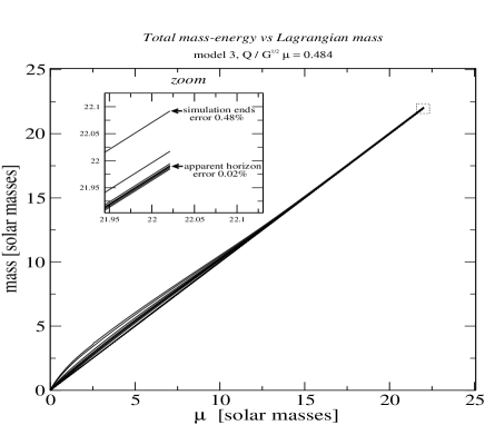
Figure 13: Snapshots for the mass-energy versus $\mu$ for model 3. The numerical error in the simulation of the models can be measured by the failure of the curves to converge at the same point, this is indicated on the zoom boxes. After the apparent horizon formation the error is $0.02\,\%$ for model 3 and model 13. The same error is found for model 13 using a lower number of radial points (see text for details). Compare with Fig. (14).

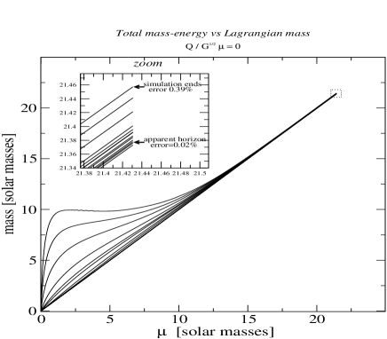
Figure 14: Snapshots for the mass-energy versus $\mu$ for model 13. The numerical error in the simulation of the models can be measured by the failure of the curves to converge at the same point, this is indicated on the zoom boxes. After the apparent horizon formation the error is $0.02\,\%$ for model 3 and model 13. The same error is found for model 13 using a lower number of radial points (see text for details). Compare with Fig. (13).

It is possible to compare the profile of the mass-energy function for the charged collapse with very strong shocks (model 3) Fig. (13), with the case of uncharged collapse (model 13) Fig. (14). The inset box of the Fig. (13) shows a zoom of the right end of the curves which indicates the level of energy conservation in the simulation. All curves must reach the same point for perfect energy conservation. At the moment of the apparent horizon formation the mass-energy is conserved with a precision of $99.98\,\%$, which is an excellent value taking into account that this is the worst case. After the apparent horizon formation, the good conserving property is lost as in any relativistic code, and the simulation is ended with a $0.48\,\%$ error. We emphasize that this is the physical quantity we use to check the convergence properties of our code, since the momentum constraint is conserved exactly by the algorithm. As was said before the simulations were performed using $1000$ points, and the conservation can be better using a larger number of points. The Fig. (14) represents the energy conservation for the case of uncharged collapse. The precision is roughly the same as in the former case, although using only $100$ points. We checked that using $1000$ points the errors are lowered by a factor of $10$ in this case, i.e.: $99.998\,\%$ precision at the apparent horizon formation. The reason for better conservation of the energy constraint is that there are not very strong shocks like in the former simulations.

The explanation of the shell formation can be grasp from the equation of motion (Eq. III). This effect can also happen in Newtonian physics, but its evolution in the strong field regime is highly non-linear and far from obvious. It seems difficult to make a complete analytic description of its evolution. However, starting with a ball of constant rest mass density and charge, it is easy to see that a shell must be formed. The relativistic term $G\,Q^{2}/c^{2}\,R^{3}$, in the Eq. (III), produce a repulsion of the matter on the initial homogeneous sphere, which in turn produce a charge gradient ${QQ_{,\mu}}/{4\,\pi\,R^{4}}$.

The term ${QQ_{,\mu}}/{4\pi R^{4}}$ in the equation of motion can be important in supporting the weight of the star (see Eq. III). Near the surface of the star, the pressure gradient term $P_{,\mu}$ cancels the charge gradient term ${Q\,Q_{,\mu}}/{4\,\pi\,R^{4}}$ at a certain point we call $\mu_{0}$. Since at this point the two terms cancels out, all the matter outside the layer of coordinate $\mu_{0}$ is almost in free fall, producing an accumulation of matter and giving rise to the shell, while at coordinates with $\mu<\mu_{0}$ the matter is supported by a positive net gradient. We took care to check that this is not a numerical artifact, changing the boundary conditions at the surface, the amount of charge, and the initial conditions.

Hence, it results that the point $\mu_{0}$ is roughly the locus in quo the term $P_{,\mu}(\mu_{0})$ and the term ${QQ_{,\mu}}/{4\pi R^{4}}(\mu_{0})$ sum zero, then the gas is compressed and a shell of matter forms.

The non-linearity in the strong field regime comes from the fact that $\Gamma$ is a function of the charge and the mass and multiplies the two gradient terms, enhancing the effect (see Eq. III).

From all the numerical experiments we performed, we observed that the shell formation effect arise more clearly when the initial density profile is flat. For the case of charged neutron star collapse the effect is negligible ghezzi2 .

The point $\mu_{0}$ shift to lower values with time, and this brings the shell to enlarge until $\mu_{0}=0$, when it reaches the origin and rebounds forming the shock wave mentioned above. It is observed that the shock do not form in the uncharged case, using the same set of initial conditions. The density contrast between the shell and its interior is higher for greater total charge (or equivalently higher internal electric field and zero total charge). This is because the Coulomb repulsion inside the shell will be higher, and this gives a higher compression of the matter at the shell. The Coulomb repulsion term together with the pure relativistic term $a{GQ^{2}}/{c^{2}R^{3}}$ in the Eq. (III), are responsible for the positive mass density gradient near the coordinate origin. The charged collapse is slightly delayed respect to the uncharged one, i.e.:$\sim 0.75$ sec for model 1 respect to the uncharged case that lasts $\sim 0.66$ sec. At the end of the simulation, we observe that the density profile looks globally flatter and the maximum density value is lower than in the uncharged case.

The case 14 in Table I is special because it represents stars with a charge greater or equal than the extremal value. We verified that in this cases the star expands “forever”, i.e.: we follow its expansion until the density gives a machine underflow. In any of these cases we expect a re-collapse of the matter: the binding energy per nucleon tends to zero when the charge tends to the mass (see ghezzi2 ), and is negative for a charge greater than mass.

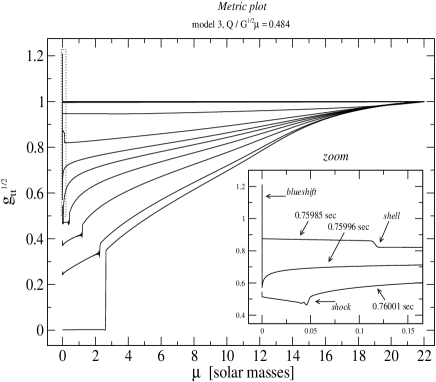
Figure 3: Snapshots of the coefficient $g_{tt}^{1/2}$, it is distinguished a sharp discontinuity at the shock and shell positions. The inset shows a zoom of the dotted box, the coefficient $g_{tt}^{1/2}$ is greater than one at the instant of time the shock revert the sign of the velocity, indicating a blueshift respect to the infalling matter. The shock and the shell are indicated in this figure.

V.1 The maximum mass limit

For charged stars there must exist a maximum mass limit like for uncharged compact stars. For white dwarfs the limit is known as Chandrasekhar mass limit, while for neutron stars is the Oppenheimer-Volkoff limit, etc. In this section, we calculate the mass limit for Newtonian charged compact stars. We assume, for simplicity, an equation of state dominated by electrons ,

$$P/\rho=Y_{e}kT/m_{B}+K_{\gamma}Y_{e}^{\gamma}\rho^{\gamma-1}\,.$$ (35)

For a spherical configuration, the Newtonian hydrostatic equilibrium gives:

$$P_{c}/\rho_{c}=GM/R-Q^{2}/(4\pi R^{4}\rho)\,.$$ (36)

Simplifying the two equations, for $T=0$ and $\gamma=4/3$ we get $(GM^{2}-Q^{2})/M^{4/3}=KY_{e}^{4/3}$. From this equations, we obtain the limiting mass $M_{max}$. Assuming the charge is a fraction $\alpha$ of the mass, i.e.: $Q=\alpha\sqrt{G}M$,

$$M_{max}=\biggl{(}\frac{K}{G(1-\alpha^{2})}\biggr{)}^{3/2}Y_{e}^{2}\sim 5.83\frac{Y_{e}^{2}}{(1-\alpha^{2})}M_{\odot}\,,$$ (37)

which reduces to the known Chandrasekhar mass formula when $\alpha=0$ (no charge), modulo some geometric factor depending on the density profile.

For the extreme case $\alpha=1$, the configuration disperse to infinity. We checked that this also happens in the relativistic case (see model 14 of Table I).

V.2 Implications for core collapse supernovae

The quantity of energy deposition behind the formed shock wave is critical to produce a successful supernova explosion, like in the proposed mechanisms for core collapse supernovae explosions colgate , Bethe , wilson . In the cases we studied the shock wave is not fast enough to reach the surface of the star before the apparent horizon forms ahead of it, and the shock ends trapped by the black hole region. However, when including neutrino transport in our simulations the shell formation could have a dramatic effect.

This provide a new mechanism for a successful core collapse supernova explosion. Although, the calculations performed in the present work are far from a complete supernova calculation, it is simple to show that in the charged collapse there are a more efficient energy deposition to revive the supernova shock wave.

As the density profile is flatter than in the uncharged case, the neutrino-sphere and gain radius for neutrino deposition must be different. In order to show this, we consider the change in the radius $R_{\nu}$, of the neutrino sphere, which is defined by $\tau(R_{\nu})=2/3$, where the optical depth of the uncharged matter for the neutrinos is Bethe

$$\tau(R)=1.5\times 10^{11}\,(N^{2}/6A)\,\epsilon_{\nu}^{2}\,R^{-2}.$$ (38)

According to the numerical results presented, we make the approximation $\rho\sim constant$, for the charged case, in order to obtain an analytic expression for the optical depth for neutrinos. In this case, the optical depth of the charged matter is

$$\tau_{ch}(R)=10^{-8}\,(N^{2}/6A)\,\epsilon_{\nu}^{2}\,\rho_{12}\,(R_{s}-R).$$ (39)

It can be seen that $\tau_{ch}\gg\tau$. Assuming typical values Bethe : $\epsilon_{\nu}=10$ Mev and $\rho\sim 2\times 10^{10}\,{\rm g\,cm}^{-3}$, in the uncharged case the position of the neutrino-sphere is at: $R_{\nu}\sim 110$ km, and in the charged case it is: $R_{\nu}\sim 845$ km. This implies a more efficient neutrino trapping during the charged collapse, and hence a more efficient energy deposition.

Table 1: Simulations of the collapse of a massive star varying the charge to mass ratio and the binding energy.

Simulation	charge to mass ratio	$\epsilon$	Binding energy	collapse ?	shell ?
	$Q/\sqrt{G}\,m$	[${\rm ergs}/c^{2}$]
1	$0.484$	$9.61\times 10^{-7}$	$-2.994\times 10^{-2}$	yes	yes
2	$0.484$	$1.92\times 10^{-6}$	$-2.992\times 10^{-2}$	yes	no
3	$0.484$	$2.88\times 10^{-6}$	$-2.990\times 10^{-2}$	yes	no
4	$0.484$	$1.44\times 10^{-3}$	$+2.498\times 10^{-4}$	no	no
5	$0.484$	$1.35\times 10^{-3}$	$-1.764\times 10^{-3}$	no	no
6	$0.145$	$1.15\times 10^{-6}$	$-3.830\times 10^{-2}$	yes	no
7	$0.145$	$9.61\times 10^{-8}$	$-3.833\times 10^{-2}$	yes	no
8	$0.145$	$9.61\times 10^{-9}$	$-3.833\times 10^{-2}$	yes	yes
9	$0.290$	$9.61\times 10^{-7}$	$-3.583\times 10^{-2}$	yes	no
10	$0.290$	$9.61\times 10^{-8}$	$-3.584\times 10^{-2}$	yes	yes
11	$0.290$	$9.61\times 10^{-10}$	$-3.585\times 10^{-2}$	yes	yes
12	$0.850$	$9.61\times 10^{-7}$	$-1.073\times 10^{-2}$	yes	yes
13	$0$	$9.61\times 10^{-7}$	$-3.740\times 10^{-2}$	yes	no
14	$\geq 1.0$	$\dots$	$\dots$	no	no

VI Final Remarks

We have performed relativistic numeric simulations for the collapse of spherical symmetric stars with a polytropic equation of state and possessing a uniform distribution of electric charge. We have not studied in this paper how the matter acquires a high internal electric field before or during the collapse process.

In the present model we studied the essential features of the collapse of stars with a total electric charge. The simulations are an approximation to the more realistic problem of the temporal evolution of an star with an strong internal electric field and total charge zero. This model is under consideration by the authors.

In the cases were the stars formed an apparent horizon it is unavoidable the formation of a Reissner-Nordström black hole. This is guaranteed by the singularity theorems and by the Birkhoff theorem.

For low values of the charge to mass ratio $Q/\sqrt{G}M\ll 1$, no difference with the collapse of an uncharged star was found. The value of the total charge that prevent the collapse of the star with any initial condition is given by a charge to mass ratio $Q/\sqrt{G}M\geq 1$. That means that stars with $Q/\sqrt{G}M\geq 1$ spreads and do not collapse to form black holes nor stars in hydrostatic equilibrium. It is observed a dramatically different physical behavior when $Q/\sqrt{G}M>0.1$. In this case, the collapsing matter forms a shell-like structure, or bubble, surrounding an interior region of lower density and charge. The effect is due to the competence between the Coulomb electrostatic repulsion and the attraction of gravity. This effect must occur in non-relativistic physics as well. The relativistic case is more interesting due to the non-linearity of the Einstein equations. The effect is more important when lower is the internal energy of the star (see Table I). In some of the experiments we observe a blueshift produced at the bouncing shock wave (see Fig. 3), because the strong shock wave acquires a positive velocity over a small lapse of time.

For all the cases studied, the density profile is globally flatter than in the uncharged collapse.

The optical depth for neutrinos is much higher in the case of the charged collapse, hence, the neutrino trapping must be more efficient. In conclusion, if the internal electric field increase during the stellar collapse the formation of the shell must be taken seriously in supernova simulations.

In addition, we obtained the mass limit formula for Newtonian charged stars, which clearly precludes the formation of naked singularities. The mass limit can not be naively extrapolated for the relativistic case, because charge and pressure regeneration effects can change the maximum charge to mass ratio. However, in the present work, we checked that it is not possible to form an star from matter with a charge to mass ratio greater or equal than one in agreement with our mass formula and with the cosmic censorship conjecture.

A more complete simulation including neutrino transport, and other quantum effects, is being considered by the authors.

References

- (1) Absoft Fortran compiler, www.absoft.com.
- (2) P. Anninos and T. Rothman, Phys. Rev. D 65, 024003 (2001). W. Israel, Phys. Rev. Letters, 57, 4, 397 (1986).
- (3) J. D. Bekenstein, Phys. Rev. D 4, 2185 (1971).
- (4) J. Bally and E. R. Harrison, ApJ 220, 743 (1978).
- (5) H. A. Bethe, ApJ 412, 192 (1993).
- (6) D. G. Boulware, Phys. Rev. D 8, 2363 (1973).
- (7) S. A. Colgate and R. H. White, ApJ 143, 626 (1966).
- (8) J. E. Chase, Il Nuovo Cimento, LXVII B, 2 (1970).
- (9) A. J. Chorin and J. E. Marsden, The mathematical introduction to fluid mechanics, Second Edition, (Springer-Verlag, New York, 1990).
- (10) J. A. de Diego, D. Dultzin-Hacyan, J. G. Trejo, and D. Núñez, astro-ph/0405237.
- (11) F. de Felice, S. M. Liu and Y. Q. Yu, Class. and Quantum Grav. 16, 2669 (1999).
- (12) A. S. Eddington, Internal Constitution of the Stars (Cambridge University Press, 1926).
- (13) C. R. Ghezzi and P. S. Letelier in “The Tenth Marcel Grossmann Meeting: On Recent Developments in Theoretical and Experimental General Relativity, Gravitation and Relativistic Field Theories” , edited by Mário Novello, Santiago Pérez Bergliaffa and Remo Ruffini (World Scientific, Singapore, 2006); C. R. Ghezzi and P. S. Letelier, gr-qc/0312090.
- (14) C. R. Ghezzi, “Relativistic Structure, Stability and Gravitational Collapse of Charged Neutron Stars”, Phys. Rev. D 72, 104017 (2005); C. R. Ghezzi, gr-qc/0510106.
- (15) N. K. Glendenning, Compact Stars (A&A Library, Springer-Verlag New York Inc., 2000), p. 82.
- (16) P. Goldreich and W. H. Julian, ApJ 157, 869 (1969).
- (17) W. Israel, Phys. Rev. Letters 57, 397 (1986).
- (18) J. D. Jackson, Classical Electrodynamics (John Wiley & Sons, New York, 1975), p. 24.
- (19) P. S. Joshi, Global Aspects in Gravitation and Cosmology (Oxford Science Publications, New York, 1996).
- (20) L. D. Landau and E. Lifshitz, The Classical Theory of Fields (Addison-Wesley Publishing Company, Inc., Reading, Massachusetts, 1961).
- (21) Lahey Computer System Inc., www.lahey.com.
- (22) P. S. Letelier and P. S. C. Alencar, Phys. Rev. D 34, 343 (1986).
- (23) B. Mashhoon and M. H. Partovi, Phys. Rev. D 20, 2455 (1979).
- (24) M. M. May and R. H. White, Phys. Rev. 141, 4 (1966).
- (25) M. M. May and R. H. White, Methods in Computational Physics 7, 219 (1967).
- (26) C. W. Misner and D. H. Sharp, Phys. Rev. 136, B571 (1964).
- (27) Herman J. Mosquera Cuesta, A. Penna-Firme, and A. Perez-Lorenzana, Phys. Rev. D 67, 087702 (2003).
- (28) E. Olson and M. Bailyn, Phys. Rev. D 12, 3030 (1975).
- (29) E. Olson and M. Bailyn, Phys. Rev. D 13, 2204 (1976).
- (30) J. R. Oppenheimer and H. Snyder, Phys. Rev. 56, 455 (1939).
- (31) B. Punsly, ApJ 498, 640 (1998).
- (32) E. Poisson and W. Israel, Phys. Rev. Letters 63 1663 (1989).
- (33) S. Ray, A. L. Espindola, M. Malheiro, J. P. S. Lemos, and V. T. Zanchin, Phys. Rev. D 68, 084004 (2003).
- (34) S. Rosseland, MNRAS 84, 308 (1924).
- (35) R. Ruffini, J. D. Salmonson, J. R. Wilson, and S. -S. Xue, A & A 359, 855 (2000); A & A 350, 334 (1999).
- (36) Y. Oren and T. Piran, Phys. Rev. D 68, 044013 (2003).
- (37) J. Schwinger, Phys. Rev. 82, 664 (1951).
- (38) S. L. Shapiro and S. A. Teukolsky, Black Holes, White Dwarfs, and Neutron Stars (John Wiley & Sons, 1983).
- (39) V. F. Shvartsman, Soviet Physics JETP 33, 3, 475 (1971).
- (40) K. A. Van Riper, ApJ 232, 558 (1979).
- (41) S. Vauclair and G. Vauclair, Ann. Rev. Astron. Astrophys. 20, 37 (1982).
- (42) A. I. Voropinov, V. L. Zaguskin, and M. A. Podurets, Soviet Astronomy 11, 442 (1967).
- (43) R. Wald, General Relativity, (University of Chicago Press, 1984).
- (44) S. Weinberg, Gravitation and Cosmology: Principles ans Applications of the General Theory of Relativity, (John Wiley & Sons, New York, Chichester, Brisbane, Toronto, Singapore, 1972).
- (45) J. R. Wilson, in Numerical Astrophysics, edited by J. M. Centrella, J. M. LeBlanc, and R. L. Bowers (eds.) (Jones & Bartlett, Boston, 1985 ), p. 422.
- (46) Ya. B. Zeldovich and I. D. Novikov, Stars and Relativity, edited by K. S. Thorne and W. D. Arnett (Dover Publications, Inc., Mineola, New York, 1971), Vol. 1, p. 451.