Exploring Halo Substructure with Giant Stars. VI. Extended Distributions of Giant Stars Around the Carina Dwarf Spheroidal Galaxy — How Reliable Are They? (astro-ph/0503627)

Abstract

The question of the existence of active and prominent tidal disruption around various Galactic dwarf spheroidal (dSph) galaxies remains controversial. That debate often centers on the nature (bound versus unbound) of extended populations of stars claimed to lie outside the bounds of single King profiles fitted to the density distributions of dSph centers. However, the more fundamental issue of the very existence of the previously reported extended populations is still contentious. We present a critical evaluation of the debate centering on one particular dSph, Carina, for which claims both for and against the existence of stars beyond the King limiting radius have been made. Our review includes a detailed examination of all previous studies bearing on the Carina radial profile and shows that among the previous survey methods used to study Carina, that which achieves the highest detected dSph signal-to-background in the diffuse, outer parts of the galaxy is the Washington $M,T_{2}$ + $DDO51$ filter approach from Paper II in this series, which depends on the stellar surface gravity sensitivity of the $DDO51$ filter to remove the bulk of contaminating foreground stars and leave predominantly stars on the Carina red giant branch. The second part of the paper addresses statistical methods used to evaluate the reliability of $M,T_{2},DDO51$ surveys in the presence of photometric errors and for which a new, a posteriori statistical analysis methodology is provided. This analysis demonstrates that the expected level of contamination due to photometric error among the photometrically-selected candidate Carina giant sample stars in Paper II is no more than 13–27% — i.e., only slightly higher than originally predicted in Paper II. In the third part of this paper, these statistical methods are tested by new Blanco + Hydra multifiber spectroscopy of stars in the $M,T_{2},DDO51$-selected Carina candidate sample. The results of both the new a posteriori and the previous Paper II contamination predictions are generally borne out by the spectroscopy: Of 74 candidate giants with follow-up spectroscopy, the $M,T_{2},DDO51$ technique successfully identified 61 new Carina members, including 8 stars outside the photometrically defined King profile limiting radius. In addition, among a sample of 29 stars that were not initially identified as candidate Carina giants but that lie just outside of our selection criteria, 12 have radial velocities consistent with membership in Carina, including 5 extratidal stars. The latter shows that, if anything, the Paper II estimates of the Carina giant star density outside the King limiting radius may have been underestimated. Carina is shown to have an extended population of giant stars extending to a major axis radius of $40\arcmin$, i.e., 1.44 times the nominal King limiting radius. A number of bright blue stars are also found to have the radial velocity of Carina and we discuss the possibility that some of them may be part of the Carina post-asymptotic giant branch population. A few additional radial velocity members are found to lie among stars in the horizontal branch and anomalous Cepheid regions of the Carina color-magnitude diagram.

1 Introduction

1.1 The Search for Extratidal Stars around dSph Satellites

The question of the stability and response of satellite dwarf spheroidal (dSph) galaxies to the Milky Way tidal field has remained a central issue in the studies of these systems since Hodge’s (1964) early discussion of tides in the Ursa Minor system. The question bears not only on the properties of these satellites — e.g., their mass, dark matter content, shape, internal dynamics, substructure, etc. — but also potentially on their role in supplying material for the continuing growth of their parent systems. Finding populations of dSph stars now unbound from their parent would certainly provide definitive evidence of ongoing stellar mass loss — presumably through tidal stripping — while measuring the rate and location of stars leaving the dSph are important gauges of the mass ratio of the dSph to the Milky Way (e.g., Hodge 1964; more recently, Moore 1996; Burkert 1997; Johnston, Sigurdsson, & Hernquist 1999, 2002) as well as the stellar accretion rate of the Galaxy. However, with the exception of the impressive and now well-studied Sagittarius dSph system, measurements of such “extratidal” populations emanating from nearby dSph galaxies has proven difficult to undertake and the results of such studies difficult to interpret. The outlying regions where the putative stripping occurs are at extremely low surface brightness levels (typically $\Sigma_{\rm V}>31$ mag arcsec^-2), and the mere detection of extratidal debris against a significant Milky Way foreground remains a daunting technical prospect.

Nevertheless, extratidal RR Lyrae stars were first reported around the Sculptor dSph by van Agt (1978), and the suggestion that there were extratidal Sculptor stars was supported by studies of other Sculptor tracer stars by Eskridge (1988a), Irwin & Hatzidimitriou (1995, “IH95”), Westfall et al. (2000), Walcher et al. (2003, “W03”) and Westfall et al. (2005). A review of the literature finds at least one report of potential “extratidal stars” around every Milky Way dSph: Sextans (Gould et al., 1992), Fornax (Eskridge, 1988b), Draco (Smith, Kuhn, & Hawley, 1997; Kocevski & Kuhn, 2000), Leo II (Siegel, Majewski, & Patterson, 2000), Leo I (Sohn, 2003), Ursa Minor (Martínez-Delgado et al., 2001; Palma et al., 2003), Sagittarius (see summary of sources in Fig. 17 of Majewski et al., 2003), and, of course, around the Carina dSph (see §1.2). In their comprehensive, systematic, photographic starcount study of Milky Way dSphs, IH95 found suggestions of excesses of stars beyond the nominal limiting radius of almost every Galactic dSph (and suggested that Sextans and Sculptor were the best candidates for tidally disrupted systems among the dwarfs they studied).

Beyond the difficulties of mere detection, determining just exactly what any discovered excesses of “extratidal” stars are also remains a challenging problem. Often the term “extratidal” is invoked to mean stars beyond the King ‘tidal’ radius of one-component models fitted to the density profile of the system; the limiting radii of fitted King functions are sometimes attributed to true tidal boundaries because of the similarity in appearance of at least some dSph radial profiles to that of tidally-truncated systems. However, a number of recent surveys (see references in previous paragraph) have found beyond the King profile-like central components of dSphs the presence of additional, extended components having a more gradual (e.g., power law) radial density decline. Such two-component density profiles are generated naturally in N-body models of the tidal disruption of satellite galaxies where the second population, outside of where the density profile “breaks”, corresponds to unbound tidal debris particles (e.g., Johnston et al., 1999; Mayer et al., 2002). However, although tidally-truncated, King-like profiles have remained useful descriptors of the inner structures of dSph galaxies for quite some time (e.g., Hodge, 1961a, b), there is no good reason to be fitting actual King (1962; 1966) functions to systems with such long crossing times, and in some cases more gradually declining (e.g., exponential) functional forms than King functions have been reported to yield equally suitable fits to the entire density profiles of Galactic dSphs (Faber & Lin 1983, IH95, Aparicio, Carrera, & Martínez-Delgado 2001; Odenkirchen et al. 2001b; Palma et al. 2003, W03). Even in systems for which King functions are appropriate descriptors, e.g., globular clusters, the King limiting radius may only be an approximation to the true, instantaneous Roche limit (e.g., King, 1962; Johnston et al., 2002; Hayashi et al., 2003), which, for example, naturally varies in position at different phases of eccentric orbits (i.e., as a function of position in the Galactic potential). Thus, even in the simplest interpretations of the structure of dSph galaxies the actual state — bound or unbound — of stars beyond the King limiting radius is not clear a priori, and any use of the expression “extratidal” in this paper is meant only to signify that stars lie beyond the single fitted King limiting radius, not that the stars are unbound.

Moreover, it is not clear whether any dark matter in these dSph systems actually follows the light profile. Indeed, the possibility of multi-component structures within dSph systems is central to the debate over the meaning of “extratidal excesses” as well as the mass-to-light ratios of these systems. The possibility that the “extratidal” excesses of stars are only a second population of dSph stars that actually lie bound deeply within large dark matter halos (like those of Stoehr et al. 2002) has also been postulated (Burkert, 1997; Hayashi et al., 2003). Measuring the dynamics of stars in these “extratidal” populations should help resolve whether these excess stars are bound or unbound and whether mass follows light in dSphs (Kroupa, 1997; Kleyna et al., 1999), but doing this has proven extremely challenging, and few examples of dSph stars clearly outside the King limiting radius of their parent system having measured radial velocities yet exist, apart from those stars observed in the tails of the the Sagittarius system — for which the first substantial results have only been recently obtained (Yanny et al., 2003; Majewski et al., 2004; Vivas, Zinn, & Gallart, 2005) Although in this paper we present (§3) the first significant sample of spectroscopic observations of stars beyond the King radius of any other dSph, and although some of these data are of sufficient level of accuracy and degree of separation from the dSph core to weigh in on the issue of whether the photometrically discovered Carina “excess” stars are bound or not, we leave this particular aspect for a separate discussion (supplemented with additional data; R. Muñoz et al., in preparation). Our primary concern here is not to explain the Carina break population, but, because this point alone has been contentious, to prove that it is real.

1.2 The Carina dSph

Although the question of the extended structure of all of the dSphs (apart from Sagittarius) has remained controversial, the case of the Carina dSph has received particular attention over the past decade. A critical review of previous work on this dSph would seem in order given that the earlier three claims for a detected break population have been apparently refuted by two more recent studies. Such a review is the first goal of this paper. In the remainder of this section we summarize and compare the previous photometric studies of Carina, with a particular emphasis on assessment of background levels, the primary limitation to reliable detection of diffuse features like dSph break populations and tidal tails. In §2 we focus on the question of modeling the contamination rate of photometrically-selected dSph giant star surveys, and present a new analytical method for assessing this rate within our previous survey of Carina in Paper II. Finally (§3) we test the predictions of the three extant contamination rate analyses of the Paper II results using new spectroscopic data on a subsample of stars in the Carina field. We also report the presence of some curious blue stars in the field having Carina velocities.

1.2.1 Starcount Studies of the Carina dSph

IH95 was the first report of an excess beyond the King limiting radius of the 101 kpc-distant (Mateo 1998) Carina system (see data in Fig. 1). Using photographic starcounts to $B\sim 22$ ($R\sim 21$) in a survey encompassing $3\arcdeg\times 3\arcdeg$ areas centered on each of the Galactic dSphs, IH95 found at large radii the presence of excess stars with respect to King profiles in most cases. The IH95 discussion of this phenomenon includes consideration of the possibility that these excess stars represent tidal stripping from the parent dSph systems.

Another, more recent dSph study that employed similar starcounting techniques, but with deeper (albeit single filter) CCD data, is that of W03. We include their density profile and fitted King profile in Figure 1. Note that W03’s King profile is similar to that found by IH95, with a King limiting radius only slightly larger ($31\farcm 8$) than the $28\farcm 8$ radius of IH95. However, while claiming to find possible extratidal debris in their similar study of the Sculptor dSph, W03 actually “rule out” the existence of a Carina break population at the levels claimed by both IH95 and by Majewski et al. (2000b, “Paper II” hereafter). As W03 state, the discrepancy between their results and the IH95/Paper II surveys is “disturbing” and “difficult to explain”. Lacking more details about each survey, we cannot offer a definitive explanation for the differences in findings, but do offer several pertinent observations that highlight possibilities.

As stressed by IH95 (for example) a major challenge confronting the study of the low surface brightness outskirts of dSphs is a proper accounting of the background. Background overestimation can erase faint dSph features, whereas background underestimation can inflate or artificially produce the appearance of diffuse features in the outer parts of dSphs. In the case of the two starcount studies mentioned, the measured background levels are comparable to the density of stars from the dSph inside the King limiting radius (Fig. 1). The actual “extratidal” signal that has been reported for Carina by any survey is significantly smaller than the background that is being subtracted by either IH95 or W03. The background confronted by IH95 has actually been significantly exacerbated by background galaxies, which were not excluded from the source counts (because morphological discrimination became unreliable in their data at the magnitude limit that IH95 adopted to access large numbers of Carina stars). Although they do use morphological criteria to exclude galaxies in their survey, W03 also note that stars and galaxies are “almost indistinguishable” at the faint end of their survey; nevertheless, morphology was used to remove some 4-10% of the total sources from their Carina survey. Yet galaxy contamination can be an order of magnitude or more larger than that expected from Milky Way stars at the brightness limits of either of these studies (see, for example, Fig. 1 of Reid & Majewski, 1993). A clue that extragalactic sources may play a dominant (but unevaluated) role in the background considerations of these surveys is that although the W03 survey probes several magnitudes fainter than that of IH95, the reported background density of sources is some four times lower in the former than in the latter survey.

The signal-to-background ratio in the outer dSph density profile is critically sensitive to both potential random and systematic errors and drives sensitivity to diffuse structures: (1) One expects naively that a study with a higher mean background compared to the central dSph density should be commensurately less sensitive to diffuse features, which can become “lost” in the Poissonian fluctuations of the background. (2) Since it is typical to take as the “background level” the point in the dSph radial profile where it flattens out, a study with a higher mean background to dSph density will be less sensitive to where the profile “goes to zero”, will tend to underestimate where this happens, and will include the lost, tenuous signal of outer dSph stars as background. Both effects are especially serious in studies where the background is larger than the “extratidal” signal of interest, but mitigated by increased survey area: (1) The error in determination of the mean background, which plays a critical role in the overall reliability of the background-subtracted density profile, correlates with the inverse square root of the number of background stars used to evaluate the background density. A larger survey area provides proportionately larger numbers of background sources at the same magnitude limit. (2) A larger survey area provides an overall larger sampling of sky away from the dSph itself, thus diluting the effects of “contamination” of the background by dSph stars.

In these respects, it is interesting to note that IH95, which has a background level about 1/4 their measured central Carina density, does detect an extratidal excess beginning at about 1/15 the central density whereas W03 do not see this excess in their survey, which adopts a background at nearly 1/40 their central Carina density. The difference in findings may relate to the error in the mean of the derived backgrounds. From their analysis of the periphery of a 9 deg² survey field, IH95 claim a rather small fractional error in their background evaluation — 0.7%. W03 do not give an estimated error in their determined background level, but this would need to have been determined to better than about 3% in order to have the same absolute error as IH95 (0.02 background sources arcmin^-2), whereas the amount of assumed “dSph-free” area is smaller in their 4 deg² survey compared to the 9 deg² area of IH95. Were the Paper II Carina density profile (Fig. 1) taken at face value, it is conceivable that as much as half of the W03 “background density” — estimated from the edge of their survey field — is from Carina itself. W03 do mention the possibility that if extended dSph populations are large enough to extend to the limit of their survey area then they would overestimate the level of their background. As we show in §3, Carina stars do exist to at least $40\arcmin$ along the major axis; this circumstance alone has probably significantly contributed to an overestimate of the W03 background density, and could explain why their deeper survey did not see an extratidal feature reported by the shallower, but larger area IH95 survey.

Yet another difference between the surveys relates to the relative magnitude errors. IH95 estimate the possibility of 0.1 mag large-scale systematic errors in their photographic data; they do not give information on the random errors but at least these are expected to be relatively uniform over their photographic plates. In contrast, mosaiced surveys of CCD data are notoriously inhomogeneous due to seeing and transparency variations during observation. It is perhaps significant that W03 report 0.1 mag uncertainties in absolute brightness for their brightest stars ($V<20$) but up to 0.3 mag uncertainties among their fainter stars. Although the photometry of their CCD frames has been tied together with stars in overlap regions, this does not account for differences in the level of Eddington (1913) bias from CCD frame to CCD frame, which, with 0.3 mag errors and a steeply rising background source count, could contribute significant excess large-scale “noise” on top of the Poissonian fluctuations. Depending on the overall uniformity of their CCD frames, the effect of variable Eddington bias may be inconsistent with the conclusion by W03 that “the precision of the photometry is not critical for this work.”

In the end it is not absolutely clear why IH95 detected an “extratidal excess” in Carina but W03 could not confirm a break to shallower slope in the Carina profile when they probed down to Carina main sequence magnitudes. It should be noted that, in spite of their repeated finding of extratidal detections around Galactic dSphs, IH95 do discuss background underestimation as one possible explanation for these (perhaps false) detections in their data, although they argue that this is unlikely for most of their dSphs. The intent of the above detailed comparison of IH95 to W03 is to demonstrate some of the pitfalls of the difficult and tedious work of deriving density profiles from starcounts and, moreover, to question the assumption in this particular kind of survey work that “deeper is necessarily better”.

1.2.2 “Filtered” Starcount Studies of the Carina dSph

W03 have used deeper imaging as one method to increase the dSph signal with respect to the background noise under the operative philosophy that the dSph signal rises faster than the increase in contributed background noise as one probes to fainter magnitudes. An alternative approach to increasing the $S/N$ of diffuse dSph features is to work hard on beating down the size of the contributed background noise by identifying and selectively weeding out those sources most likely to be unrelated to the dSph. If multifilter data are in hand, one can use the fact that dSphs have well-defined loci in the color-magnitude diagram to eliminate a large fraction of the background sources inconsistent with membership in the dSph. The method of counting stars lying in well-chosen regions of the color-magnitude diagram (CMD) where the target signal-to-background noise ratio is optimized has been applied to the search for tidal tails around globular clusters by Grillmair et al. (1995, 1996); Leon, Meylan, & Combes (2000); Rockosi et al. (2002), and Odenkirchen et al. (2001a, 2003), around dSph galaxies by Kleyna et al. (1998) and Piatek et al. (2001), as well as to searches for tidal tails in the Galactic halo (Martínez-Delgado et al., 2001, 2002; Bellazzini et al., 2003; Ibata et al., 2003). In a variant of this technique, Kuhn, Smith, & Hawley (1996) fitted the CMDs of extratidal fields around the Carina dSph with combinations of “Carina” and “background” CMD templates, and found a radial profile break population with a density roughly consistent with those found by IH95 and Paper II. Because this information is not available from their paper, we cannot include the Kuhn et al. relative Carina-to-background density in Figure 1, but it is expected to be better than that of IH95. More recently, Monelli et al. (2003) have reported a “shoulder” in the density distribution of stars selected from regions in the Carina CMD meant to be dominated by old Carina stars (the RR Lyrae, BHB and subgiants), and suggest it may be related to the predicted Johnston et al. (1999) radial profile “break” in tidally disrupting systems; however, this Monelli et al. break occurs well inside the King radius (4-6 arcmin from the center of Carina) and its relation to the data from other surveys shown in Figure 1 is unclear. On the other hand, in a more recent contribution, Monelli et al. (2004) report the likely presence of the old Carina MSTO in a CMD for a field located just outside of the Carina tidal radius, a result that supports the notion of a true break population there.

To improve the signal-to-noise ($S/N$) of the tenuous extratidal features even further, Paper II added to the optimized CMD filtering technique an additional strategy to identify and remove residual “noise” that happens to fall within the selected regions of the CMD. Because this residual “background noise” is actually dominated by foreground Galactic disk dwarf stars, Paper II relied on a photometric method that can discriminate them from Carina giant stars: The Washington $M,T_{2}+DDO51$ filter technique (Geisler, 1984; Majewski et al., 2000a) relies on the surface gravity sensitivity of the Mgb+MgH spectral features near 5150Å in late G- and K-type stars (the feature is secondarily sensitive to metallicity). The result of this two step filtering technique is a drastic reduction of the background level and the resultant detection of a very obvious break population in the distribution of Carina giant stars (Fig. 1) which is consistent with that reported by both IH95 and Kuhn et al. (1996). A benefit of the Paper II analysis is that it goes beyond a mere statistical measurement of the Carina radial profile; rather, it endeavors to identify precisely which stars are members of the dSph, and these can be spectroscopically targeted for a straightforward check of the veracity of the derived photometric profile (see §3). The technique also supplies a relatively pure target list of the most accessible stars to use for study of the dSph’s dynamics (Muñoz et al., in preparation). Figure 1 shows that of all the photometric Carina studies to date, the Paper II survey is the only one for which the identified break population is at a density greater than its subtracted background and by almost an order of magnitude, in contradistinction to the other surveys for which the inverse (or worse) is true.

Said another way, the Paper II background would have to be underestimated by almost a factor of ten in order to erase the detected break population in Paper II. Moreover, the error in that estimated background would have to show a systematic radial trend away from the center of Carina in order to create the false signal of a power-law decline in the dSph outside the nominal King limiting radius. While it would seem difficult for any analysis to have made an error in measurement both so incredibly large as well as so remarkably unfortunate as to have an inverse power-law radial variation, this is exactly the position taken by Morrison et al. (2001, “MOMNHDF”), who, through a reanalysis of the Paper II data, conclude that the detected break population is entirely an artifact of photometric errors. However, as we now show, the MOMNHDF analysis contains several errors and mistaken assumptions about the Paper II study that leads them to this incorrect conclusion.

2 Assessments of the Paper II Contamination Level

2.1 Review of Goals and Conclusions of Paper II

Paper II used the $M,T_{2},DDO51$ technique to identify an extended distribution of giant star candidates beyond the nominal “tidal radius” of the Carina dSph galaxy, a stellar excess also previously reported by IH95 and Kuhn et al. (1996). As discussed above and in these cited references, the existence of such break populations may have profound implications for the outer structure, dark matter content, disruption history, and/or perceived star formation histories of satellite dSph galaxies, as well as the structure and formation of the Milky Way halo. Paper II discussed several physical explanations for the apparent extended distribution of stars found beyond the nominal Carina tidal radius, including the possibility that Carina is losing about 27% of its mass per Gyr. As stated in Paper II, each of the various possible explanations “has a distinct, kinematical signature that would be recognizable with an appropriate radial velocity survey.” Without radial velocity data, not only were such speculations about the meaning of the Carina radial structure beyond verification, but the actual analysis of the Carina structure itself was necessarily based, in large part, on “extratidal” star candidates around which it was felt that a strong case for reliability had been built — but candidates nonetheless. Because of an inability to have made significant progress with spectroscopic testing of these candidates, despite repeated attempts over five years, the Paper II analysis of Carina relied in part on statistical arguments, including, for example, in the assessments of sources of potential contamination of the giant candidate sample. Thus, Paper II made a first attempt, via comparison of background stellar densities in regions of color-magnitude space adjacent to that region used to select Carina giant star candidates, to account for two sources of potential contamination: (1) field giants and metal-poor subdwarfs having similar $M-DDO51$ colors to the selected Carina giant sample, and (2) non-Carina stars errantly scattered into the photometrically-selected sample due to random errors in the photometry. However, Paper II did present a small-scale spectroscopic test of the accuracy of the photometric dwarf/giant separation: For a proxy sample of 27 Carina region stars for which spectroscopic data existed a 100% accuracy in the dwarf/giant classifications was found, and among these 27 stars were three newly discovered giants outside the nominal Carina tidal radius.

2.2 Review of Goals and Conclusions of MOMNHDF

Subsequently, MOMNHDF re-addressed the issues of subdwarf contamination and photometric errors in Washington$+DDO51$ surveys; their analysis relied on Monte Carlo simulation of photometric error spreading in the Washington$+DDO51$ filter color-color diagram for the latter effect. MOMNHDF include a reexamination of the contamination rate in the Paper II study of Carina, and reach dramatically different conclusions about it: As summarized in their Figure 13, MOMNHDF’s results suggest that the entire sample of “extratidal” Carina giant candidates identified in Paper II can be accounted for as contamination by misidentified subdwarfs and by photometric errors that scatter Galactic disk dwarf stars from the “dwarf” region of the $(M-T_{2},M-DDO51)_{o}$ diagram into the “giant” region. In addition, MOMNHDF discount the Paper II spectroscopic test as being relevant to assessing the veracity of that work, since they consider at least two of the spectroscopically confirmed “extratidal” giants as insufficiently outside the tidal radius to be significant (when they account for errors in the establishment of that radius by IH95).

MOMNHDF conclude: “If one wishes to make statistical corrections for the number of bogus giants caused by photometric errors, it is important to quantify accurately the photometric errors in the data, both in terms of the average error and the shape of the distribution.” This warning, as well as the general themes of the MOMNHDF paper, emphasize, appropriately, the caution one must have in any study making use of photometrically selected samples. Ironically, however, MOMNHDF themselves have inaccurately quantified both the “average error and the shape of the [Paper II error] distribution”, so that they have greatly overestimated the number of potential contaminants in the Paper II, candidate Carina giant sample. Additional simplifications and incorrect assumptions in the MOMNHDF analysis have further inflated their estimated Paper II contamination levels, as demonstrated in the following subsections. We first reexamine the MOMNHDF numerical technique (§2.3) and then introduce an alternative, and we believe more accurate, analytical method for a posteriori assessment of contamination levels (§2.4). However, through both methods we find not only much more modest levels of dwarf contamination (at levels near those calculated in the original Paper II analysis via its third, independent assessment method), but that in seeking to be conservative, Paper II might actually underestimate the density of extratidal Carina giant stars.

2.3 Numerical Simulation of Contamination Level

An ideal numerical analysis of the Paper II photometric survey along the lines of that approximated by MOMNHDF would proceed by (1) invoking a “truth” distribution, $X$, of points $\mbox{\boldmath{$x$}}_{i}$ representing both Milky Way and Carina stars in the three-dimensional space $(M-T_{2},M-DDO51,M)_{o}$ and (2) applying random deviates, $\mbox{\boldmath{$\xi$}}_{i}$ (appropriately matched to the measured error distribution in each dimension) to create a new distribution, $Y$, of perturbed points $\mbox{\boldmath{$y$}}_{i}=\mbox{\boldmath{$x$}}_{i}+\mbox{\boldmath{$\xi$}}_{i}$, in the three-dimensional space. After perturbation of the truth sample by one level of error, (3) the number of stars that cross the three-dimensional “Carina-giant candidate” selection boundaries of Paper II (in either direction) may be evaluated. With Monte Carlo methods for selecting the random deviates, (4) the process may be repeated multiple times to evaluate an expected mean level of dwarf contamination of the “Carina-giant candidate” sample.

Unfortunately, a number of unavoidable factors make it difficult to realize this “ideal” methodology, but MOMNHDF have in addition made some (avoidable) simplifications that have a critical impact on their assessment of Paper II. Here we discuss various points pertinent to a MOMNHDF-like numerical simulation of the Paper II photometric errors:

$\bullet$ Picking an appropriate truth sample. To implement the “ideal” numerical simulation of the effects of errors on the experiment requires the adoption of a suitable representation of an errorless data distribution. Unfortunately, the truth distribution $X$ is ultimately unknown, and may only be approximated by an observed distribution, $X^{\prime}$, where each point is already perturbed by one level of error, $\mbox{\boldmath{$x$}}_{i}\rightarrow\mbox{\boldmath{$x$}}_{i}+\mbox{\boldmath{$\xi$}}_{i}^{\prime}$. Thus, any numerical experiment where the number of error-perturbed dwarf stars becoming giant contaminants is evaluated that starts with an observed dataset must be acknowledged a priori to overestimate the amount of that contamination. Clearly, the smaller the $\mbox{\boldmath{$\xi$}}_{i}^{\prime}$, the more reliable the approximation to the truth distribution. For the simulation they show in their Figure 7, MOMNHDF have taken a “dwarf locus” from their own survey, after imposing a severe 0.02 magnitude error limit in each magnitude, so that, in general, $\overline{|\mbox{\boldmath{$\xi$}}_{i}^{\prime}|}<<\overline{|\mbox{\boldmath{$\xi$}}_{i}|}$ for each star in their simulation. This seems a reasonable simplification for their simulation only because MOMNHDF have assumed $\overline{|\mbox{\boldmath{$\xi$}}_{i}|}=0.10$ mag; however, as we show below, this is not at all typical of the errors in the Paper II sample, which are more like 0.033 mag. For a large fraction of the stars in the Paper II sample, the $\overline{|\mbox{\boldmath{$\xi$}}_{i}^{\prime}|}$ MOMNHDF adopted in their Figure 7 simulation are relatively close to the $\overline{|\mbox{\boldmath{$\xi$}}_{i}|}$ of Paper II. The situation is, however, even worse for the MOMNHDF analysis of “giants kept/dwarfs gained” (their Figs. 8 and 9) since here the authors have imposed no error limit on their “zero error” input data set.

Even were one to adopt an essentially “zero-error” (but observed) distribution of dwarfs (or any stars) to represent the truth distribution in one direction of the sky, a second problem arises in that the truth distribution is not a constant around the sky. For example, the shape of the “dwarf locus” is a function of Galactic position because of its dependence on the metallicity distribution of those stars (see, for example, Figure 2 of Majewski et al., 2000a). MOMNHDF have taken their “zero-error” distribution from their own survey fields with latitude ranging from $25\arcdeg\leq b\leq 72\arcdeg$; however, since Carina is at $b=-22\arcdeg$, one would expect a proper “truth” distribution of dwarf stars for the Carina field to contain a metallicity distribution skewed towards higher abundance disk stars than does a high latitude sample. Because higher metallicity dwarfs lie further from the Paper II giant/dwarf separation in the two-color diagram (2CD) than do lower metallicity dwarfs, it is likely that MOMNHDF’s “zero-error” dwarf locus will admit more contaminants into the giant region than would a dwarf locus appropriate to the Carina line-of-sight.

$\bullet$ Using a three-dimensional analysis. The MOMNHDF discussion focuses on their simulation of error propagation in the $(M-T_{2},M-DDO51)_{o}$ plane. However, Paper II selected a star to be a “Carina RGB candidate” based not only on it having a position in the $(M-T_{2},M-DDO51)_{o}$ plane expected for giant stars, but also a position in the $(M-T_{2},M)_{o}$ color-magnitude plane commensurate with probable association with the Carina dSph. While the first criterion used was generally more liberal than that used by the “spaghetti group” in their own selection of giant candidates (see MOMNHDF), the second criterion was designed to be so conservative in disallowing potential Carina-RGB candidate contaminants that it more than makes up for the relatively more vulnerable color-color criterion, and it is a critical aspect of our process. For example, it is not clear why the MOMNHDF simulation of Paper II permits stars as blue as $(M-T_{2})=0.5$ and why the authors focus on this “blue extension [that] causes problems” since application of the various Paper II CMD selection criteria significantly reduces or entirely eliminates this “blue extension”. Indeed, for the Paper II $M<19.3$ sample the ultimate $(M-T_{2})$ color selection is at least as strict, if not more so, than that applied by MOMNHDF in their own survey. Failure to incorporate the true Paper II color limits has substantially inflated the number of “MOKP [Majewski et al. (2000a)] bogus giants” demonstrated in MOMNHDF’s Figure 7, for example. It is the three-dimensional aspect of the Paper II selection criterion, i.e., that a star must land in a very restricted volume of $(M-T_{2},M-DDO51,M)_{o}$ space, that makes its ultimate selection of candidates so conservative. Moreover, as shown below, the larger mean density of stars inside this parameter space selection volume compared to the density just outside of it means that it is statistically more likely for bona-fide Carina RGB stars to be scattered out of the small selection volume in parameter space than for non-Carina-RGB stars to enter it, even when photometric errors as large as 0.1 mag per filter (those invoked and studied by MOMNHDF) are allowed.

$\bullet$ Assuming Gaussian deviates. As pointed out by MOMNHDF, the detailed shape of the error distribution can play an important role in the outcome of a numerical simulation. In the face of no information to the contrary, it is common (and generally easy) to assume that the distribution of errors is Gaussian. Obviously, the wings of a platykurtic error distribution will produce more spurious contaminants, while a leptokurtic distribution will yield fewer problems. We have checked the shape of the Paper II error distribution through an analysis of the errors in the magnitude distributions of artificial stars and find that the MOMNHDF assumption of a Gaussian shape to the Paper II error distribution is valid.

$\bullet$ Assuming a proper-sized distribution for the Gaussian errors. A fundamental problem with MOMNHDF’s critique of Paper II is that the level of error they have adopted to represent the photometric sample in the evaluation of the number of potential contaminants is too large. MOMNHDF’s criticism of the Carina giant candidate selection might be well-founded if indeed the typical photometric errors were as large as 0.1 mag; however, 0.1 mag is the magnitude cut-off applied in the Paper II analysis, and can hardly be considered the typical magnitude error. Obviously, attributing the worst photometric error (0.1 mag per filter, or 0.14 error per color) to the entire sample of Paper II stars grossly exaggerates the degree of smearing of the dwarf locus (as represented in MOMNHDF’s Figs. 4 and 13) and results in a greatly overestimated number of contaminants scattered into the giant selection region in $(M-T_{2},M-DDO51)_{o}$ space. MOMNHDF’s conclusions that the Paper II “extratidal” population may be entirely due to dwarf star contamination, which they obtain from the simulation results summarized in their Figure 13, can only be reached after applying this maximum photometric error in the Paper II sample to all stars.

Even then the apparent convergence of their worst case, 0.15 mag color error models to a 100% contamination within the extratidal Carina giant sample shown in MOMNHDF’s Figure 13 is incorrect because MOMNHDF have undercalculated/mislabeled the density of extratidal giants that Paper II identified as 100 deg^-2, when the actual density that Paper II reported is 124 deg^-2. The mistakenly reported lower density value likely derived from having used the entire area of the Paper II survey to calculate the extratidal density (i.e., 1.16 deg²), and neglecting to exclude the area in the intratidal region (0.22 deg²). This 23% underestimate also affects the background (i.e., contaminant) density that they report from Paper II: The actual “MOPKJG [Paper II] background estimate” is 27.9 deg^-2, not the 22.5 deg^-2 MOMNHDF show.

As shown by Figure 2, the reality of the Paper II error distribution is far less pessimistic than the strawman, “photographic quality”, error distribution that MOMNHDF have criticized: The median errors in the deepest, $M=20.8$ sample of Paper II are at $\sigma_{M}=0.033$ mag, $\sigma_{M-T_{2}}=0.045$ and $\sigma_{M-DDO51}=0.050$. Therefore, it is worthwhile assessing what MOMNHDF would have concluded from their own analysis had they accounted for the actual error distribution in the Paper II data: For the actual median Paper II color error of $\sim 0.0475$ mag, the MOMNHDF model results as presented in their Figure 13 yields an expected number of “interloper dwarfs” among the extratidal Carina giant candidates much smaller than MOMNHDF have implied, and, moreover, very near what the original Paper II analysis estimated them to be — i.e. about 30 deg^-2!

However, the latter simple comparison ignores the potentially deleterious effects of the small number of stars with larger than typical photometric errors in the asymmetric wing of the error distribution — the problem objects more similar to the kind (but not proportion) MOMNHDF simulated. Thus a better assessment of what MOMNHDF’s model would predict in the case of the true photometric error distributions comes by finding the expectation value of the product of their Figure 13 interloper function with our Figure 2 error distributions. Because MOMNHDF present results (their Fig. 13) only in the case for equal errors in all magnitudes, whereas the actual data have varying errors in each dimension of $(M-T_{2},M-DDO51,M)_{o}$ space, for our calculation we adopt from the MOMNHDF Figure 13 a fractional interloper expectation for each star inferred from the abscissa point given by the geometric mean of the axial radii of the error ellipsoid, $2^{1/2}(\sigma_{M}\sigma_{T_{2}}\sigma_{DDO51})^{1/3}$, where the $2^{1/2}$ comes from the fact that MOMNHDF’s Figure 13 presents results in terms of color, not magnitude, error. For the $M=20.8$ sample (the case presented in MOMNHDF’s Figure 13), we find that MOMNHDF’s model with the actual error distribution of the Paper II sample gives a density of photometric error contaminants of 22 deg^-2. When one adds in the 14 predicted metal-poor subdwarfs from their model, one gets 36 total contaminants – again, rather similar to the total contamination level of 28 deg^-2 calculated in Paper II. The relatively close agreement between the MOMNHDF model results using the proper Paper II error distribution and what we derived for the net contamination of the Carina giant candidate sample from the very different analysis in Paper II suggests that the adoption of inflated photometric uncertainties is the predominant shortcoming in MOMNHDF’s analysis.

$\bullet$ Measuring the missed detection rate. MOMNHDF concentrated on the number of “bogus” sources entering into the Carina giant sample. However, without also including a distribution of Carina giants in their simulation, MOMNHDF did not address the possibility of sample flux in the other direction — i.e., a loss of true Carina stars from the sample. For stars near the three-dimensional selection boundary, the volume of parameter space available to stars leaving the selection volume is larger than for stars that would scatter into the comparatively small selection volume. Thus, MOMNHDF’s, as well as our previous, estimates of the degree to which the Paper II extratidal densities are inflated by photometric errors ignores a potentially significant countereffect that reduces measured Carina densities relative to the background (indeed, even increasing the background level as estimated by the methodology of Paper II), making the the derived extratidal giant densities more conservative.

2.4 Analytical Estimation of Contamination Level

MOMNHDF’s evaluation of sample contamination employs a model of the data to numerically simulate the effects of photometric errors. In this subsection we describe an alternative, analytical, a posteriori approach to ascertaining sample contamination levels by using the data themselves. With it we reaffirm the independent Paper II analysis of the level of contamination in our final “Carina giant candidate” sample, which is significantly less than proposed by MOMNHDF.

The number of stars scattered into our three-dimensional $(M-T_{2},M-DDO51,M)_{o}$ Carina giant selection due to photometric errors can be assessed by considering the probability distribution function for the colors and magnitudes of individual stars. What we calculate for each giant candidate is the posterior probability that it belongs inside the giant selection region. This calculation assumes that the giant selection region that we have employed separates giants from dwarfs with perfect accuracy, which is the simplest assumption one can make for now; when additional information becomes available (e.g., through an empirical determination of the true contamination rate via spectroscopic observations of a large sample of our giant candidates) the assumption about the accuracy of our giant selection region can be adjusted (see §2.4.1).

Each star identified as a candidate Carina giant by our combined color-color and color-magnitude selection process has an associated photometric error in each filter, $\sigma_{M}$, $\sigma_{T_{2}}$, and $\sigma_{DDO51}$. These quantities can be used to compute a covariance matrix for the magnitude, $M$, and the colors $M-T_{2}$ and $M-DDO51$, which represents the total error in the position of a star within the three-dimensional color-color-magnitude space. The covariance matrix can be written as

$$[C]=\left[\begin{array}[]{ccc}\sigma^{2}_{M}&\sigma^{2}_{M}&\sigma^{2}_{M}\\ \sigma^{2}_{M}&\sigma^{2}_{M}+\sigma^{2}_{T_{2}}&\sigma^{2}_{M}\\ \sigma^{2}_{M}&\sigma^{2}_{M}&\sigma^{2}_{M}+\sigma^{2}_{DDO51}\end{array}\right],$$ (1)

where only the terms involving $\sigma^{2}_{M}$ survive in the off-diagonal terms because the errors in different magnitude terms are uncorrelated.

Assuming that the photometric errors in each filter have a Gaussian probability distribution, then the likelihood that each star, $i$, has an $(M-T_{2})^{\prime}$ color, $(M-DDO51)^{\prime}$ color, and $M^{\prime}$ magnitude different from its measured values, $(M-T_{2})_{i}$, $(M-DDO51)_{i}$, and $M_{i}$, is

$$L(M-T_{2}^{\prime},M-DDO51^{\prime},M^{\prime})=\frac{1}{(2\pi)^{3/2}\,\sigma_{M}\,\sigma_{T_{2}}\,\sigma_{DDO51}}\exp\left(-\frac{1}{2}x^{2}\right),$$ (2)

where

$$x^{2}\equiv[\Delta]^{T}[C]^{-1}[\Delta],$$ (3)

and $[\Delta]\equiv[M^{\prime}-M_{i},(M-T_{2})^{\prime}-(M-T_{2})_{i},(M-DDO51)^{\prime}-(M-DDO51)_{i}]$. Using Bayes’ theorem, the probability that each star is either a giant or a contaminant becomes

$$P([M-T_{2}]^{\prime},[M-DDO51]^{\prime},M^{\prime})=\frac{L([M-T_{2}]^{\prime},[M-DDO51]^{\prime},M^{\prime})*P_{0}([M-T_{2}]^{\prime},[M-DDO51]^{\prime},M^{\prime})}{D},$$ (4)

where $P_{0}([M-T_{2}]^{\prime},[M-DDO51]^{\prime},M^{\prime})$, known as the prior, is the a priori probability (based on the information $I$) that we would consider each star a contaminant, and $D$ is a normalization factor chosen such that the integral of $P([M-T_{2}]^{\prime},[M-DDO51]^{\prime},M^{\prime})$ over all possible values of $M$, $M-DDO51$ and $M-T_{2}$ is one.

2.4.1 An Aside About Prior Probabilities

In order to evaluate equation (4) above, we must write an expression for the prior, $P_{0}([M-T_{2}]^{\prime},[M-DDO51]^{\prime},M^{\prime})$. The proper choice of this quantity is often a subject of heated debate in discussions of Bayesian methods. In fact, a properly chosen prior should rarely make a significant difference in the final results. To see why this is so, consider the strategies by which a prior might be chosen.

First, we might choose an “uninformative prior”; that is, a prior that makes weak assertions about the a priori distribution of the variables being measured. Priors typically used for this purpose include the uniform prior, $P(X)=\mbox{\rm constant}$ and the Jeffreys’ prior, $P(X)\propto 1/X$. When using a prior of this sort, the posterior probability will be dominated by the contribution of the likelihood function. In essence, we “forget” our a priori assumptions once we have actual measurements in hand.

Alternatively, we might choose an “informative prior.” This would be especially appropriate, for example, if there were an accepted value derived from previous experiments for the quantity under investigation. In this case the prior and the likelihood ought to agree. If they do, then the effect of the prior is to tighten the confidence intervals around the peak of the posterior distribution; this is equivalent to a meta-analysis of the data from all of the experiments. If the prior and the likelihood do not agree, then we should probably not be applying equation (4) blindly; we should instead figure out the reason for the discrepancy.

For this study the probability density in the color-color-magnitude space is probably not uniform, but we are reluctant to choose an informative prior unless it can be rigorously defended, which in practice means we limit our use of informative priors to meta-analysis. Accordingly, we adopt the uniform prior for these calculations, and equation (4) becomes

$$P([M-T_{2}]^{\prime},[M-DDO51]^{\prime},M^{\prime})\propto L([M-T_{2}]^{\prime},[M-DDO51]^{\prime},M^{\prime}),$$ (5)

with the constant of proportionality set by the normalization condition.

2.4.2 Contamination Evaluation

Let $R$ denote the giant selection region of ($M-T_{2}$, $M-DDO51$, $M$) space, and $\tilde{R}$ its complement. Then the probability, $P_{i}$, that a star, $i$, belongs in $\tilde{R}$ and not in $R$ is

$$P_{i}=\int_{\tilde{R}}P([M-T_{2}]^{\prime},[M-DDO51]^{\prime},M^{\prime})\>d(M-T)^{\prime}\>d(M-D)^{\prime}\>dM^{\prime}.$$ (6)

The integral in equation (6) is difficult to evaluate analytically because the boundaries are irregularly shaped; consequently, we use a Monte Carlo integration technique (e.g., Press et al., 1992, §7.6), in which $\int fdV\approx V\langle f\rangle$, where $f$ is a function and $V$ is the parameter space volume over which we are integrating. We generate integration sample points using a quasi-random sequence (Press et al., §7.7). Although the integral extends formally to infinity in the ($M$, $M-T_{2}$, $M-DDO51$) space, for practical reasons we impose a bounding box, which we make large enough that $P_{i}$ is negligible along the boundary for all stars in the sample. The integration samples span the entire ($M-T_{2}$, $M-DDO51$, $M$) space within the box, but only those in $\tilde{R}$ are allowed to contribute to the integral. Then, the volume of $\tilde{R}$, $V_{\tilde{R}}$, is given by $(N_{\tilde{R}}/N_{\rm tot})V_{\rm tot}$, where $(N_{\tilde{R}}$ is the number of integration samples within $\tilde{R}$, and $N_{\rm tot}$ is the total number of samples. The expectation value for the number of $\tilde{R}$ stars that appear in $R$ due to photometric error is then

$$\langle N_{c}\rangle=\sum_{i=1}^{n}P_{i}.$$ (7)

There are two sources of uncertainty in $\left\langle N_{c}\right\rangle$. The first is the error in the approximation to the integral in equation (6). The Monte Carlo technique used to evaluate the integral is a numerical approximation, and the sampling error, $\sigma_{MC,i}$, in this approximation for each star $i$ is given by $\sigma^{2}_{MC,i}=V^{2}(\langle f_{i}^{2}\rangle-\langle f_{i}\rangle^{2})/N$. The total variance in $\left\langle N_{c}\right\rangle$ from these errors is then $\sigma^{2}_{MC}=\sum_{i}\sigma^{2}_{MC,i}$.

The second source of uncertainty is the statistical uncertainty inherent in any random experiment; viz., the number of contaminants actually observed will not be exactly $\left\langle N_{c}\right\rangle$, but will instead have some probability distribution peaked at $\left\langle N_{c}\right\rangle$. We can calculate the variance of this distribution by considering the two possibilities for each star found in the selection region. Either the star is a true Carina giant ($c=0$), or the star is a contaminant ($c=1$). If the star’s contribution to $\left\langle N_{c}\right\rangle$ is $\mu=P_{i}$, then the variance contributed is

$$\sigma^{2}_{i}=\sum_{c=0,1}\left[(c-\mu)^{2}P_{i}(c)\right],$$ (8)

or

$$\sigma^{2}_{stat}=\sum_{i}\sigma^{2}_{i}=\sum_{i}P_{i}(1-P_{i}),$$ (9)

since $P_{i}(c=0)=1-P_{i}$ and $P(c=1)=P_{i}$. Finally, the combined uncertainty from both effects is $\sigma_{\langle N_{c}\rangle}=\sqrt{\sigma_{MC}^{2}+\sigma_{stat}^{2}}$.

The statistical uncertainty is fixed for any particular sample; however, the error in the numerical approximation is a function of how many points are sampled in the integration, and can be reduced to insignificance. The Monte Carlo integration was carried out with 10,000,000 integration samples, so that $\sigma_{\rm MC}\lesssim 1/4\sigma_{\rm stat}$ in the majority of cases. Test calculations were run with the number of integration samples ranging from 25,000–10,000,000 and with integration limits extending to $12<M^{\prime}<25$, $-2<(M-T_{2})^{\prime}<6$, and $-1.0<(M-DDO51)^{\prime}<1.0$. Other than the expected decrease in $\sigma_{\rm int}$ due to the increase in integration samples, the resulting number of contaminants remained constant through the various trials; thus, the contamination estimates are insensitive both to the number of points used in the integral approximation and to the limits of integration.

In Table 1 we report the expected number of contaminants found in various subsamples of candidate giant stars drawn from the catalogue of all stars observed in our survey of the Carina dSph. Various subsamples are used to determine whether the rate of contamination is significantly larger at faint magnitudes or in the extratidal region than it is at bright magnitudes or in the core of the galaxy. The integration was carried out over a finite region of parameter space that included all values of $(M-T_{2})^{\prime}$, $(M-DDO51)^{\prime}$, and $M^{\prime}$ that might possibly contribute to the integral: The adopted ranges are $14<M^{\prime}<23$, $-1<(M-T_{2})^{\prime}<5$, and $-1.0<(M-DDO51)^{\prime}<1.0$.

The subsamples evaluated include the four magnitude-limited subsamples in Paper II ($M\leq 19.3,19.8,20.3,20.8$), with and without the Paper II imposed 0.1 mag photometric error limit on the dataset. Table 1 shows that the contamination fraction in every subsample is not a major fraction of the total sample of Carina giant candidates. The calculations show the highest level of contamination ($\sim$44%) is predicted in the subsample of extratidal Carina giants with no photometric error limits applied and with a magnitude cut of $M\leq 20.8$; this is expected because this subsample includes the largest fraction of stars with errors potentially large enough to scatter stars into the Carina giant region. In every case, when we apply the actual Paper II photometric error limit (i.e., $\sigma_{M},\sigma_{T_{2}},\sigma_{DDO51}\leq 0.1$) the expected level of contamination drops, but not by huge fractions (e.g., for the $M\leq 20.8$ extratidal sample, from 60 out of 137 to 48 out of 118, or from 44% to 41%). For the entire sample of giant candidates with 0.1 mag error limits, depending on the magnitude limit, the contamination level is expected to be about 13% to 27%. These levels of predicted contamination are clearly not the 100% proposed by MOMNHDF.

While these calculated estimates of the amount of contamination of our giant candidate sample due to photometric error may still seem large, they may also be overestimated. The calculation that has been performed is only applicable to the determination of the number of objects that truly lie outside our giant selection region that we “incorrectly” designate as giants. However, the criteria used to select Carina giants is not perfect; it was designed to be conservative in its selection of stars as Carina giants in order to mitigate the amount of contamination, and in so doing, it purposely excludes other types of expected Carina members. It is very likely that many of the objects found just outside our giant selection region are Carina asymptotic giant branch (AGB) stars, Carbon stars, horizontal branch (HB) stars, etc. Thus, objects found outside the box that scatter into the box are not necessarily non-Carina members (see, e.g., §3.3.2). Moreover, just as non-Carina stars may be scattered into the giant selection region due to photometric error, the opposite also occurs: Carina giants are scattering out of our giant selection region due to photometric error. The combination of these two effects implies that the contamination levels reported in Table 1 should be taken as upper limits.

Finally, we note that the analysis presented here accounts only for stars misclassified as Carina giants due to photometric error. It does not address the issue of how well the boundaries of the three-dimensional selection region separate Carina giants from other non-Carina stars that should lie within the giant selection region (e.g., field halo giants or extreme subdwarfs with colors and magnitudes that happen to place them along the Carina locus). On the basis of the radial velocity (RV) distributions of the Carina giant sample (§3 and Figure 4a below) it is possible that these types of contaminants (which might be assumed to have Galactocentric RVs relatively far from $0\,{\rm km\,s^{-1}}$ — but not necessarily so; see §3.4) make only a small contribution to the total contamination. It is worth noting that an accounting of this type of contamination is expected from the methodology for subtracting “background” described in Paper II.

MOMNHDF claim that the majority of the extratidal giant candidates identified in Paper II are misclassified dwarfs due to (their large adopted) photometric errors, while the results presented here suggest that only a fraction of these candidate Carina giants can be misclassified stars. As shown in Table 2, the true detection fraction of actual Carina giants predicted by our new analytical method (column 4) are generally smaller than, but in keeping with, the general fractions estimated in Paper II (column 5). As one more verification that the major source of the difference between the results of the MOMNHDF simulation and our own calculations here lies in their adopted error distribution, we assigned each star in our sample an error in the three filters of $\sigma=0.1$, the value used in MOMNHDF, and repeated our computation of the expected number of contaminants among the sample of 118 extratidal giant candidates with $M\leq 20.8$ from Paper II. The result of assuming errors this large is that we should expect $68\pm 5$ contaminants (compared to the 48 expected contaminants calculated using the proper error distribution). This number, when normalized for the survey area covered by the $M\leq 20.8$ extratidal sample, is $59\pm 5$ deg^-2. This is still smaller than, but more consistent with, the value of 85 deg^-2 misclassified dwarfs that MOMNHDF estimate our contamination would be were the error in each filter for every star as large as 0.1 mag.

2.4.3 Ranking Giant Candidates

The probability calculation just described was used to determine the number of expected contaminants in the Paper II samples of giant candidates; however, the calculation also provides a method for estimating a likelihood that any particular star is a Carina giant (and the method can of course be generalized to the study of other star systems). $P_{i}$ provides a measure of how closely the $(M-T_{2},M-DDO51,M)_{o}$ of star $i$ match those of a typical Carina giant star, taking into account photometric error, and can be used to rank stars from most likely Carina giants ($P_{i}=0$) to least likely Carina giants ($P_{i}=1$). Astrometrists use a similar technique in the proper motion vector point diagram of star cluster fields (see e.g., Cudworth, 1985), with cluster membership probability assigned to each star by comparing its proper motion and error to that of the cluster mean, and even more sophisticated joint (trivariate) probabilities that also account for location of the star in the cluster CMD as well as the spatial location of the star with respect to the cluster center have been adopted (see, e.g., Galadí-Enríquez, Jordi, & Trullols, 1998). A sample of giant candidates selected using stars in limited ranges of our trivariate photometric membership probabilities, $P_{i}$, should be more representative of the true distribution of Carina giants, and identify the best Carina candidates for spectroscopic verification. Once spectroscopy is in hand, one may also explore probability trends in the contamination level as a function of different parameters in order to refine future selection criteria.

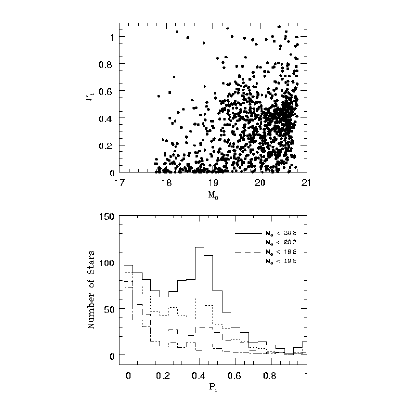
Figure 3: (Top) Distribution of the probability of being a contaminant, $P_{i}$, as a function of $M$ magnitude. (Bottom) Distribution of $P_{i}$ for the four magnitude limits adopted in Paper II.

For example, while in the end MOMNHDF, commenting on the Paper II Carina survey, admit that “brighter [giant candidate] stars, such as the three [sic] observed spectroscopically, will have smaller photometric errors and will in general be giants if they are in the giant region”, there remains a legitimate concern about the level of contamination at fainter magnitudes. However, Figure 3, which shows the determined $P_{i}$ as a function of $M_{o}$, suggests that mean calculated probability of being a contaminant grows relatively slowly with magnitude. The maintenance of a more similar error distribution with magnitude is partly a reflection of Paper II’s progressive removal of bad data with each increasedmagnitude limit.

It should be kept in mind that the $P_{i}$ scale is dependent on the exact shape of the selection boundary and is only a rank order metric internal to a particular survey. Moreover, $P_{i}$ reflects the probability of contamination within the adopted selection boundary — it does not, strictly speaking, say anything about the true probability of being a Carina giant. The degree to which $P_{i}$ does reflect the probability of being a giant relies on the degree to which the triavariate selection boundary genuinely separates Carina giants from non-giants, but this surface is difficult to know a priori. From this standpoint, therefore, the $P_{i}$ should be looked on only as a guide to the relative likelihood of membership from star to star.

3 Spectroscopic Assessment of Carina Giant Membership

3.1 Observations and Reductions

In Paper II we had access to a total of 27 stars in the Carina field having spectroscopic data from either Mateo et al. (1993) or our own observations, among which were 21 Carina giants and 6 field dwarfs. Our photometric selection criteria correctly classified all of them. Nevertheless, one might be concerned (as suggested by MOMNHDF) that a higher contamination rate in our candidate sample might be expected at lower Carina densities. In addition, MOMNHDF considered the three spectroscopically-confirmed stars in Paper II that are outside the tidal radius to be insufficient evidence that we are finding an extended/extratidal Carina population.

Since Paper II we have continued spectroscopic follow-up of our Carina giant candidates, more than tripling the number with spectra and, as a further test of our procedures, observing many more stars in the Carina field not selected to be Carina giants. Here we focus on what the derived radial velocities (RVs) of these stars tell us about our photometric selection methodology. Further consideration of the dynamics of the outer parts of the Carina system are presented elsewhere (R. Muñoz et al., in preparation).

Spectra of our Carina giant candidates have been obtained using the Blanco 4-m + Hydra multifiber spectrograph system at Cerro Tololo Inter-American Observatory on the nights of UT 2000 March 26-29, 2000 November 10-12 and 2001 October 8-11. In all runs the region around the calcium infrared triplet was observed. For the year 2000 runs, the Loral 3K$\times$1K CCD and grating KPGLD in first order was used; this set-up delivers a resolution of $\sim$2600 (or 2.6Å per resolution element). For the October 2001 run, we used the SITe 4K$\times$2K CCD and grating 380 in first order and also inserted a 200 $\mu$m slit plate after the fibers to improve the resolution to $\sim$7600 (1.2Å per resolution element).

Our strategy for targeting stars with fibers was to place as first priority those stars that were selected to be Carina giants. Remaining fibers were filled with stars not picked as Carina giant stars as a means to assess the level of “missed” Carina giants with our photometric selection criteria. Among these “fiber filler stars” observing priority was given to stars that were picked as giants stars in the 2CD but outside the Carina RGB selection box in the CMD. Another category of filler stars were those also lying just outside the 2CD giant star boundary (for which we eventually obtained good spectra of six). Finally, because of the potential that they might be halo HB stars or HB/anomalous Cepheid stars from Carina, we also targeted stars bluer than the main sequence turn-off of the field star population in the CMD. Any still unused fibers were placed on blank sky positions to obtain at least a half-dozen background sky spectra. Four unique Hydra pointings of Carina targets were obtained in March 2000 and two unique pointings in November 2000; for these runs 64 fibers were available for both target and sky observations (fibers not able to be used for any stars are generally used to collect background sky spectra). For the October 2001 run, we obtained two unique Hydra pointings, each observed on two different nights, with 133 available fibers. Multiple observations of the same set-up as well as cross-targeting of individual stars in the Carina field between different set-ups allows a check on the RV errors (random and systematic) for individual stellar targets (Table 3). To aid the RV calibration, multiple (6 to 13) RV standards were observed each run, where each “observation” of an RV standard entails sending the light down 7-12 different fibers, yielding many dozen individual spectra of RV standards. For wavelength calibration, the Penray (HeNeArXe) comparison lamp was observed for every fiber setup.

Preliminary processing of the two-dimensional images of the fiber spectra was undertaken using standard IRAF techniques as described in the IRAF imred.ccdred documentation. After completing the bias subtraction, overscan correction and trimming, the images were corrected for pixel-to-pixel sensitivity variations and chip cosmetics by applying “milky flats” as described in the CTIO Hydra manual by N. Suntzeff.

Spectral extraction across the PSF of the individual fibers made use of a local IRAF script much like imred.hydra.dohydra, but developed to simplify Hydra reduction for our RV analysis. The script is based on standard IRAF spectroscopic reductions using imred.hydra.apall for extraction of the fibers, and imred.hydra.identify and imred.hydra.reidentify for wavelength calibration of the comparison spectra. The wavelength solutions are applied using imred.hydra.refspec and then dispersion corrected to a common wavelength range with imred.hydra.dispcor. Finally, a master sky spectrum is made and subtracted from the target stars using the noao.onedspec.skytweak task.

Our RV reduction is a modified version of the classical cross-correlation methodology of Tonry & Davis (1979). However to improve the velocity precision, we pre-process the spectra by Fourier filtering and, for the RV template spectra, filtering in the wavelength domain to remove those parts of the spectra that contribute little to the cross-correlation template other than noise. To do so, the filtered template is multiplied by a mask that is zero everywhere except at a set of restframe wavelengths of low ionization or low excitation transitions of elements observed in moderately metal deficient stars. The latter process leaves only the most vertical parts of relatively strong spectral lines to provide the cross-correlation reference. It is found that very strong lines that are not on the linear part of the curve of growth, like the Ca II infrared triplet, are not as useful in this enterprise, and these lines are actually left out of our cross-correlation. Since the output of the correlator is affected only by the strength of the selected spectral feature compared to that in the master, this manufactured template spectrum is fairly insensitive to spectral type. The Fourier-filtered and masked template, when correlated with the Fourier-filtered target stars, only responds to spectral lines that have been selected when they are present. If a selected template spectral line is absent in the target star what little effect is introduced from photon noise is free of bias and detracts minimally from the correlation. The foundations and application of this cross-correlation methodology are described more fully in Majewski et al. (2004).

A quality factor (see Majewski et al., 2004) is assessed for each derived stellar velocity depending on the strength and shape of the correlation peak with respect to other features in the cross-correlation function, with $Q=7$ being a solid RV measurement and $Q=4$ the lowest quality cross-correlation that yields a trustworthy RV (albeit at lower precision for these typically $S/N\sim 5-6$ spectra than for those with higher $Q$). By comparing multiple measures of the same star among the numerous RV standard observations we have found typical dispersions of $5\,{\rm km\,s^{-1}}$ for the KPGLD grating setup (year 2000 observations) and $2\,{\rm km\,s^{-1}}$ for the 380 grating setup (year 2001 observations). Because the spectra of the Carina stars are of lower $S/N$, we adopt errors twice the above values as representative RV errors among the higher quality ($Q=6$ or 7) Carina targets. As we show below (Tables 3 and 4), these assumed RV errors are not unreasonable.

An unfortunate aspect of this observing program was that it faced consistently mediocre to poor observing conditions, with each run having significant clouds and/or poor seeing. This prevented us from obtaining good $S/N$ spectra for every targeted star, and generally only the brightest stars in each fiber set-up had spectra with enough $S/N$ to derive reliable RVs ($Q>3$); the results for these stars are presented in Tables 3, 4 and 5. As may be seen, the number of successfully observed Carina targets is substantially less than the many dozens targeted across the eight different fiber set-ups (generally about 75% of the available 64 or 133 total fibers per set-up). Originally we sought four to five hour exposures per set-up, but actual integration times ranged from 1.5 to 3.5 hours because of frequent shutdowns for weather and technical problems, and these exposures, of course, were generally compromised with clouds or poor seeing. The large variation in integration time is the reason there are few multiply observed stars from October 2001 (Table 3), even though each fiber set-up was observed twice on this observing run.

On the other hand, because these spectra have been obtained with fibers feeding a bench-mounted spectrograph we should not face the same problems with variable and uncertain entrance aperture illumination and mechanical flexure that is common to slit spectroscopy; thus we might not expect to be quite as haunted by systematic RV shifts from observing run to observing run, or pointing to pointing. We have noted before (Majewski et al., 2004) that our initially derived RVs face some systematic offset from true RVs due to the detailed structure of the manufactured RV cross-correlation template. The value of this small offset is derived by the difference between the measured and literature RV values of the numerous RV standards observed. After application of the derived systematic offsets from run to run, we cannot discern a plausible offset between the RV systems of those fiber setups that have stars in common (Table 3). As one demonstration of this fact, the entries for each star in Table 3 are listed in RV order, whereas the dates of the observations do not have any consistency in their relative ordering from star to star.

For stars observed multiple times, the adopted radial velocities (final entries in Table 5) represent weighted averages, $<RV>$, of the individual measured velocity values, $v_{i}$, given in Table 3 for that star:

$$<RV>=\sum_{i}(\omega_{i}^{2}v_{i})/\sum_{i}(\omega_{i}^{2}).$$ (10)

The weighting factors take into account the fact that the spectra have different $S/N$ while two spectral resolutions are represented among the data. For purposes of weighting, we adopt the system-wide values of $10\,{\rm km\,s^{-1}}$ and $4\,{\rm km\,s^{-1}}$ as representative relative velocity errors, $\epsilon_{i}$ between the lower and higher resolution spectra, respectively, and obtain weights as

$$\omega_{i}=\omega_{quality,i}\times(1/\epsilon_{i}).$$ (11)

Previous experience shows that the actual velocity precision is inversely related to the height of the cross-correlation peak ($CCP$), but not necessarily in a linear fashion. Therefore we adopt the following additional factors in the weighting: $\omega_{\rm quality,i}$ = 0.5/1.0/2.0/3.0 for RVs with $CCP$s in the ranges ($<$0.3)/(0.3-0.5)/(0.5-1.0)/($\geq$1.0).

Table 3 gives the standard deviation, $s(RV)$, of multiply-measured stars, and reveals that in general the standard deviations are consistent with the representative RV errors adopted above — namely 4 and $10\,{\rm km\,s^{-1}}$ errors for the higher and lower resolution data for spectra with higher quality (i.e., higher $CCP$ and $Q$). Typically in those cases where $s$ substantially exceeds the above representative values, at least one of the measures is of lower quality, as might be expected. In one case (star C1394) where $s$ is extremely large one of the two measures is right at our minimum level of acceptable quality, and this quality is evidently overestimated.

A comparison of our Hydra RVs to previously published values for stars in common with Mateo et al. (1993) and Paper II is given in Table 4. For the stars C1547 and C2282 we obtain RVs within a few ${\rm km\,s^{-1}}$ of the Mateo et al. values. For star C2774 our RV is $17\,{\rm km\,s^{-1}}$ different than that of Mateo et al., but this Hydra RV also has a relatively low $CCP$ and $Q$, so the difference is not surprising. We have also remeasured with Hydra the four stars with du Pont telescope spectra (having typical RV errors of $10-15\,{\rm km\,s^{-1}}$) presented in Paper II. The new spectra are both of higher resolution and better $S/N$, so here the comparison provides a less useful quantitative evaluation of the new data. However, it is interesting to note that for two of the du Pont-observed stars (C2501583 and C2103156) the new Hydra RVs are much closer to the canonical Carina RV. The other two Paper II stars have consistent RVs between du Pont and Hydra.

Table 5 summarizes the Hydra results for all stars in the Carina field having spectra with high enough Hydra $S/N$ to derive reliable RVs, or that have been published before by Mateo et al. (1993). The entries include the star name, fiber coordinates, date observed (for Hydra observations), photometric data (dereddened values), and the derived heliocentric RV ($V_{\rm r}$), $CCP$ and RV quality ($Q$) values for each star (we denote RVs derived from Mateo et al. with a $Q=M$). The column “Cand” in Table 5 specifies whether the star was originally selected to be a Carina giant (“Cand” = “Y”) or not (“Cand” = “N”). The Table 5 sample of 134 stars includes 74 stars selected as candidate Carina giants using the Paper II criteria and 60 “fiber filler” stars including six known dwarf stars from Mateo et al. (1993). The final column in Table 5, “Mem?”, summarizes our evaluation of the true membership to the Carina system according to the procedures outlined below.

3.2 Defining Carina RV Membership

Armed with new RV data, we must determine a method by which to judge what is a Carina member. Fortunately, at Carina’s position in the Galaxy (near the direction of anti-rotation, $[l,b]=[260.1,-22.2]^{\circ}$) and systemic heliocentric velocity ($V_{\rm r}=223.1\,{\rm km\,s^{-1}}$; Mateo 1998), the random non-Carina stars in the field should be dominated by stars having substantially different RVs than Carina. Among the stars selected to be giant candidates, the primary expected contaminants will be: (1) stars errantly selected due to photometric errors, which are presumably dominated by the more populous foreground disk dwarfs and which will be obvious by their near zero RVs, (2) metal-poor dwarfs with low magnesium abundances, which at the survey magnitudes will be dominated by Galactic thick disk stars, and which will (given the asymmetric drift of this Galactic population) have RVs somewhere between that of thin disk stars and Carina, but closer to the former, and (3) random halo giants not related to Carina. If the Galactic halo is randomly mixed and has close to zero net rotation, the mean halo giant velocity in the Carina direction will, in fact, have a heliocentric RV close to that of Carina, but the broad velocity dispersion of a dynamically hot halo ($\sim 100-150\,{\rm km\,s^{-1}}$; e.g., Norris, Bessell, & Pickles, 1985; Carney & Latham, 1986; Layden et al., 1996; Sirko et al., 2004) means that only a fraction of these stars will have RVs lying within the tighter range of Carina stars. On the other hand, if the halo is instead not well-mixed and networked with dynamically cold substructures, there is the possibility of both large density variations in “field giant” density as well as the potential for other substructure in the field with any particular mean velocity (e.g., see §3.4), including, in principle, one near that of Carina. But overall, from these general arguments, we conclude that RVs should provide a fairly reliable means to discriminate Carina members from non-Carina stars in the same field.

Figure 4 gives RV histograms of all 134 stars in Table 5. The distributions of stars selected photometrically as Carina giant candidates (Fig. 4a) and those not selected to be Carina giant candidates (Fig. 4b) are shown separately. The clear signal of Carina stars near its systemic velocity of $\sim 223\,{\rm km\,s^{-1}}$ is obvious in Figure 4a; in general these Carina stars are fairly separated from the small fraction of stars photometrically selected to be “Carina giants” but having RVs inconsistent with Carina membership (i.e., Paper II “false positives”). The near zero heliocentric velocities for most of the latter stars suggests that the primary source of the small amount (quantified below) of contamination is the Galactic thin disk, with stars presumably making it into our sample through photometric error (however, see §3.4). Despite the rather clear delineation of Carina stars in the top panel of Figure 4, we seek a “fair” way to discriminate members versus non-members because: (1) A few stars selected as Carina giants have more intermediate RVs, which gives them “borderline” Carina membership depending on the criteria selected. (2) We are also interested in possible Carina membership among the “filler star” sample (Fig. 4b), which spans a larger RV range. Among the latter, there is a peak in the RV distribution at the Carina systemic RV, indicating the presence of a fair number of Carina stars. We can use the appearance of the Carina RV distribution in the top panel to guide how Carina members among the filler stars might be identified.

To select stars as Carina RV members objectively, we determine the mean value of the “Carina peak” in Figure 4a using an iterative rejection of 2.5$\sigma$ outliers. In terms of the number of $\sigma$, this is more restrictive than the $3\sigma$ limit utilized by, for example, Wilkinson et al. (2004) in their study of the Ursa Minor and Draco dSphs, but in terms of absolute velocities it is larger because the latter work had better, $2.4-2.9\,{\rm km\,s^{-1}}$ RV precision. However, while we are forced to accept a broader absolute RV range to accommodate our larger intrinsic RV errors, we can “afford” to do this because we have vetted our stars to be photometrically-selected giants and a comparison of Figure 4a to Figure 4b shows that this step must be at least partly effective in lowering contamination. The primary expected contaminant with a near-Carina RV would be a halo giant star, but any giant star slipping through our photometric selection criteria with a similar RV and distance (i.e., position in the CMD) as Carina RGB stars are most likely to be Carina RGB stars. Upon convergence of the iterative procedures, those stars in Figure 4a lying within 2.5$\sigma$ of the mean, where $\sigma$ is found to be $16.6\,{\rm km\,s^{-1}}$, are kept as Carina members. Sixty-one stars remain in the converged fit, and yield a mean Carina RV of $222.8\,{\rm km\,s^{-1}}$, only $0.3\,{\rm km\,s^{-1}}$ from that found by Mateo et al. (1993) — but note that all 17 of the latter stars are included among the former. For the “filler star” sample, we adopt these same RV limits as a starting point to hunt for additional Carina members, but also explore the positions of these stars in the CMD as an additional criterion to judge for likely membership to Carina (§3.3.2 and §3.3.3).

3.3 Evaluating the Paper II Carina Giant Selection

3.3.1 Membership Rates and False Positives

The subsample of stars observed with Hydra were selected for maximal efficiency in fiber usage with the multi-object spectrograph, and among the stars observed there is uneven $S/N$ due to variable weather conditions, integration times and stellar fluxes. Therefore, this subsample is not easily described in terms of statistical completeness with regard to sky position, color, magnitude or photometric errors. As a test of our photometric survey the most straightforward assumption is that the RV sample represents a reasonable proxy of the the full Carina giant candidate list so that we may compare our expectations for the contamination level with the “false positive” fraction number among the 74 Carina giant candidates having measured RVs.

Based on the definition of Carina RV membership adopted in §3.2, we derive the fractional number of “true members” for various subsamples drawn from the Carina giant candidate sample as shown in Table 2. The spectroscopically-verified membership fraction numbers, given by the fraction of stars in Table 5 with “Cand”=“Y” that also have “Mem?”=“Y”, are compared to both the member fractions rates predicted from the analysis in §2 and to the background rates derived in Paper II. As may be seen, the actual observed rates of true Carina members among the Carina giant candidates are similar to those previously predicted here and in Paper II, and, obviously, there is nowhere near the “100% contamination” suggested by MOMNHDF. Rather, the spectroscopic membership fractions are close to, and more often than not higher than, those predicted from our analysis in §2.

Overall we find that our $M,T_{2},DDO51$ methodology is rather efficient at identifying true Carina members across the various subsamples listed (44-94% members, depending on the actual magnitude, magnitude error and spatial location limits imposed on the Paper II photometric database). The trend is for lower membership fractions among the deeper samples, presumably because of a larger fraction of stars with larger photometric errors and because the giant branch here is bluer and closer to the color of the bulk of the contaminants. Across our full survey to $M=20.8$ the spectroscopic membership rate is 81%. In comparison, for example, the Mateo et al. (1993) selection of Carina candidates proved only 74% efficient in finding true members, and this was among a sample of the very brightest ($M<18.3$, or a magnitude limit $\sim 1.0$ mag brighter than our brightest magnitude limit), reddest (i.e., most obvious compared to the field star population) candidates in the Carina core where the density of members is several orders of magnitude higher than in much of the area we have explored here.

The overall high membership rate among the Carina giant candidates is similar to — though less than — the positive results we have had with other, similar Washington$+DDO51$ selected giant candidate samples we have studied spectroscopically in this series of papers: (1) In an analysis of the Ursa Minor dSph by Palma et al. (2003) identical to the Paper II analysis of Carina, our technique is 100% accurate in classifying 84 giant stars, 60 dwarf stars, and even one field giant, among 154 spectra obtained by Hargreaves et al. (1994) and Armandroff, Olszewski, & Pryor (1995). The remaining 9 stars are found to be RV members of UMin, but they were not selected photometrically as candidate stars because the majority appear to be AGB stars, which are found just outside the adopted CMD limits of the Palma et al. RGB locus. (2) In the similar survey of Leo I by Sohn (2003) and S. Sohn et al. (in preparation), we have obtained spectroscopy of 85 Leo I giant candidates from the center and out to 1.3 times the King limiting radius and have verified 100% of them to be Leo I giants. (3) In a study of the Sculptor system (Westfall et al., 2005), we have found 97% of the 146 photometrically-selected Sculptor giants to be RV members of the dSph, including stars to 1.5 the King limiting radius. (4) As part of the program by Guhathakurta et al. (2004) Keck spectra for 30 Andromeda I giant candidates and 24 Andromeda III candidates identified with the same techniques have been obtained (J. Ostheimer et al., in preparation). All of the And I/III giant candidates are found to be RV members of these systems, apart from only two And I candidates that are M31 halo giants (which share the same RGB and distance as And I, and can hardly be considered as “failures” of our method). These results for other dSphs are additional evidence that our photometric selection method works well and that it is a most efficient way to find the “needle-in-the-haystack” giant stars needed for study of true dSph stars well outside of the core radius.

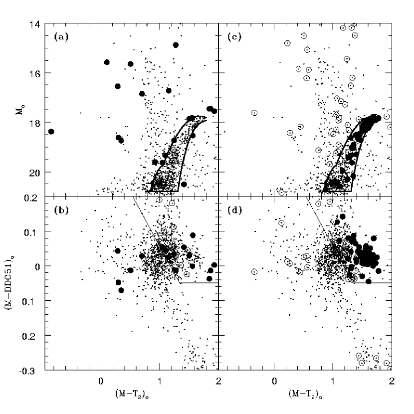
Figure 5: (a) $(M-T_{2},M)_{o}$ diagram marking the location of stars not photometrically selected as giants but with velocities consistent with being a Carina member (solid circles) and stars selected as giants but with a velocity not consistent with being a Carina member (open circles). (b) $(M-T_{2},M-DDO51,)_{o}$ diagram for the same data as panel (a). (c) $(M-T_{2},M)_{o}$ diagram showing the location of stars selected as giant candidates and confirmed spectroscopically as Carina members (solid circles) as well as stars not selected to be Carina giants having RVs inconsistent with Carina membership (open circles). (d) $(M-T_{2},M-DDO51,)_{o}$ diagram for the same data shown in panel (c). In all panels, the dots show stars within 0.2 King limiting radii (IH95) and were plotted as a guide to the general CMD features of the Carina field. The solid lines in all panels delineate the CMD and 2CD selection criteria. The dwarf stars appearing in the lower right of panel (d) are from the Mateo et al. (1993) study, and were not selected as giant stars in Paper II.

It is interesting to assess the primary source of the false positive detections. From the discussions in Paper II, MOMNHDF, and §2, and the distribution of RVs in Figure 4a (see §3.2), the expectation is that the primary source of contaminants are stars whose photometric errors are sufficient to scatter them into our selection criteria. Figures 5a and 5b show the location of the false positives (open circles) in the CMD and 2CD respectively. As may be seen, many of the stars are near at least one of the selection boundaries, but some are not, and require larger photometric errors to scatter them into our sample. The left panels of Figure 6 demonstrate that, indeed, the false positives are among those stars with larger photometric errors and, as expected, those with the highest calculated probabilities of being a contaminant. Indeed, near 100% reliability would have been found had we limited our spectroscopy to stars having photometry of a precision near the median magnitude errors ($\sigma\sim 0.035$ mag) of the Paper II survey. On the other hand, such a limitation would have missed a number of the actual Carina members found in the spectroscopic sample (about half of the stars selected with the poorer photometry are found to be Carina members), including most of the extratidal examples. The main conclusion to be drawn from the left panels of Figure 6 is that when better photometry is available the $M,T_{2},DDO51$ technique as practiced in Paper II works even better; such photometry is now available for Carina (R. Muñoz et al., in preparation). However, even with modest photometric quality, reasonable membership identification rates have been achieved.

Figure 7 shows the distribution of RVs as a function of $P_{i}$, and demonstrates the usefulness of the $P_{i}$ for identifying those stars most likely to be Carina giants ($P_{i}=0$). As $P_{i}$ increases, its discriminatory power declines, but with improved photometry and improved selection boundaries (see §3.3.2) the $P_{i}$ discrimination of Carina giants should improve.

From the standpoint of claims for extratidal giant star densities, Table 2 suggests that Paper II has, in fact, underestimated its background levels. In the worst case scenario — i.e., for our deepest samples to $M=20.8$ where the level of contamination is predicted and observed to be highest — Table 2 suggests that the true densities of Carina stars may actually be as low as 82% of the value calculated in Paper II across our entire survey area or 64% of the value calculated in Paper II for the “extratidal” regions where the results are most contentious. Nevertheless, as discussed in §1.2 and as is clear from Figure 1, raising the estimated, subtracted extratidal backgrounds accordingly (e.g., by a factor of two in the worst, $M=20.8$ extratidal case) will not erase the presence of an excess density of stars outside the nominal tidal radius of Carina. Moreover, as we now demonstrate, the existence of additional true Carina giants missed by our Paper II selection criteria means the true density of such stars is actually higher than the Table 2 numbers would imply.

3.3.2 “Missed” Carina Members

We have shown that among stars selected in Paper II to be Carina giants, a major fraction of them are indeed true Carina members. But if we are interested in evaluating the true densities of Carina giants at any given Carina radius, it is useful to understand how complete was the Carina star selection in Paper II. A lower limit to the “missed” density of Carina giants may be derived from the numbers of plausible RV giant members found among our “fiber filler” sample. The starting points for this evaluation are the potential “missed” Carina RV members shown by the shaded region in Figure 4b.

Among these, we focus first on the stars observed spectroscopically from the “fiber filler” category of stars selected to be giant stars, but that lie outside the CMD selection for Carina giants. Twenty-nine of these stars were successfully observed, and, by the RV membership criteria of §3.2, 12 of these stars have RVs in the “Carina-member” range. The CMD and 2CD distributions of these stars are shown in Figures 5a and 5b by the filled circles redward of the field star main sequence turn off (near $[M-T_{2}]_{o}=0.75$). Interestingly, all but two of these stars lie quite near the edge of the CMD selection boundary. The star with Carina-like RV near $M\sim 14.8$ (C2300060) is too bright to be part of the Carina system while the red star near $M\sim 16.8$ (C2501002) could be part of the Carina system only as some kind of post-asymptotic giant branch (PAGB) species (see §3.3.3). Of the remaining ten stars with Carina-like RVs three appear to be at the Carina AGB tip, while others fall just above and below the CMD selection box. Because of the proximity of these stars to the Carina RGB and their Carina-like RVs, these stars are almost certainly true Carina members. Inspection of the photometric errors associated with the red “fiber filler” stars (Figure 6, right hand side) indeed shows that some of these stars may have been “missed” by the Paper II Carina selection criterion because photometric errors scattered these stars out of our sample. On the other hand, some of these stars seem to have relatively good photometric uncertainties, so that it is likely they have been missed because the Paper II CMD selection criteria were too conservative. It is found that had the CMD selection limits been extended in both directions of luminosity by 0.15 mag, seven of these stars would have been selected as members, thereby increasing the completeness of the sample with virtually no change in the spectroscopic membership fractions in Table 2. In the Table 5 summary, we have marked as Carina members all red “fiber filler” candidates with Carina-like RVs and lying just outside the Carina RGB boundary in the CMD. This includes the three stars with Carina RVs above the tip of the boundary in the CMD.

A secondary filler star category is red stars just outside the selection criteria in both the 2CD and the CMD. Among the six of these stars observed, none are found to have a Carina-like RV. A seventh star falling inside the CMD selection but just outside the 2CD selection is also found not to be a Carina RV member. These results suggest that the color-color selection criterion adopted in Paper II was reasonably placed for discriminating that part of parameter space well-populated with Carina giants from that not well-populated.

3.3.3 Additional Carina Members

Another category of fiber filler stars targeted spectroscopically were blue stars. Although these do not bear directly on the efficiency of our giant star selection, it is of interest to know whether additional Carina members lie among the blue stars in the Carina field. As shown in Figure 5, eighteen blue [$(M-T_{2})_{o}<0.75$] stars have been targeted; seven of these blue stars (those with filled symbols in Figure 5a and 5b) have RVs that we have defined as Carina-like according to the criterion in §3.2. Two of the blue stars near $M\sim 18.7$ (C4156 and C2563) lie in the region of the Carina field CMD occupied by Carina anomalous Cepheids (Figure 8) in the survey by Dall’Ora et al. (2003), and these two stars have been identified as variable by these authors. Given that these two stars also lie within the Carina King limiting radius, they are almost certainly Carina members.

Recognizing that pulsating variable stars have RVs that shift tens of ${\rm km\,s^{-1}}$ from their mean velocity it is worth investigating whether there may be other Carina pulsators with RVs slightly outside the RV membership limits adopted in §3.2. Figure 9 shows the distribution of RVs for all eighteen targeted stars with $(M-T_{2})_{o}<0.75$. The distribution is more or less bimodal with one group having $V_{\rm r}$ closer to zero. Among the other nine stars, seven are tightly clumped at the nominal Carina RV, but two lie within $15\,{\rm km\,s^{-1}}$ of the lower RV-membership limit from §3.2. One of these stars (C3994) lies among the anomalous Cepheids in the CMD and the other (C3001272) lies on the Carina HB near the instability strip (both stars are marked by squares in Fig. 8); both lie well inside the Carina King limiting radius and we consider them both to be Carina members having RVs modulated by pulsation.

On the other hand, the four brightest blue stars with Carina-like RVs are too bright to be Carina anomalous Cepheids and are 4-5 magnitudes brighter than the Carina HB. Yet it is somewhat remarkable that these four stars should have such similar RVs to each other and to Carina. While it is plausible that these stars represent an unrelated moving group of halo HB stars that just happen to have the same RV as Carina, the two faintest of the four bright blue stars (C1211401 and C3897) lie within 0.7 tidal radii of the center of Carina, which represents a small fraction ($\sim$ 10%) of the total survey area. These two stars are at reasonable magnitudes to be post-AGB (PAGB) stars from Carina’s $\sim 2$ Gyr population (e.g., see PAGB evolutionary tracks from Blöcker (1995), which show that for Carina stars no younger than $\sim 2$ Gyr the PAGB can have $-4.5\lesssim M_{V}\lesssim-2.8$, or about 2.4-4.1 magnitudes above the Carina HB). This PAGB “sequence” might even extend to the redder star (C2501002, also shown in Figure 8) at the same magnitude and that also possesses a Carina RV. On the other hand, the two brightest blue stars with Carina RVs (C3509707 and C2502058) would seem to require more massive, even younger progenitors for explanation as Carina PAGB stars. Recently the existence of Carina stars as young as 0.6 Gyr or younger have been reported by Hernandez, Gilmore, & Valls-Gabaud (2000) and Monelli et al. (2003). Such stars may be sufficiently massive to create PAGB stars that approach the brightness of stars C3509707 and C2502058 (Blöcker, 1995). In addition, were the latter stars some variety of pulsational variable, it is possible that they are “caught” near maximum brightness. In this regard it is interesting to note that one of the Carina field variables identified by Dall’Ora et al. (2003) has the same apparent magnitude as the two brightest blue RV stars (see Fig. 8), although these authors actually identify this star as a 0.3 day period RR Lyrae. One other problem with the possible association of C3509707 and C2502058 to a $<1$ Gyr Carina population is that those young Carina stars are preferentially concentrated to the core of the dSph, whereas the two bright blue stars with Carina RVs are well outside the King limiting radius (see the two open squares with Carina RV in Fig. 10a). Alternative explanations that could accommodate scenarios with older populations might include that the two bright stars come from older AGB progenitors that endured less mass loss, or that they are “born-again AGB stars (e.g., Iben et al., 1983), although finding two examples of stars in such a short phase of stellar evolution would seem extremely unlikely. In the end, we regard the status of these two stars in our sample as still very uncertain. It will be interesting to obtain RVs of the other bright blue stars in the field to see if additional stars at the same magnitudes have Carina RVs, a situation that would be even harder to explain away as mere field contamination.

Finally, the bluest star for which we have obtained a spectrum (C1201) also seems to have a Carina-like RV. This star lies in a CMD position that is not inconceivable for a fading PAGB star.

In the end, it is plausible that at least seven of the nine blue stars with RVs similar to that of Carina are true Carina members (using the expanded RV acceptance range discussed above); the fainter five are marked as such in Table 5, whereas the two near $M_{o}=16.8$ are marked as “Mem?”=“Y?”. The remaining two stars might be extremely bright Carain PAGB stars, but this is unlikely because (1) their origin is challenging to explain, and (2) their position outside the nominal Carina tidal radius is incompatible with the least unlikely scenario involving an association with rather young progenitors.

3.4 A Second Look at the RV Distribution

To this point we have regarded our targeted Carina giant stars (Fig. 4a) having $V_{\rm r}\lesssim 100\,{\rm km\,s^{-1}}$ as being most likely dwarf star contamination from the Milky Way disk (and in §3.3.1, along with Fig. 6 we argued that larger photometric error among the false positives points in this direction). However, another possibility is that these stars represent giant stars from other halo substructure having these velocities. We arrive at this notion via the results of a large area, deep survey for giant stars we have conducted (see Majewski et al., 1999; Majewski, 2004) around the Magellanic Clouds and including fields within $5-10^{\circ}$ of Carina. The RV distribution of the giant stars in these fields is nearly bimodal, with one large group of stars concentrated with RVs between $100-200\,{\rm km\,s^{-1}}$ less than that of Carina (e.g., see right side of Fig. 6 in Majewski, 2004). This RV clustering of stars, which have projected giant star distances ranging to many tens of kiloparsecs, is already observed to span tens of degrees on the sky and it is not inconceivable to find this same population of stars in the relatively nearby Carina field. While in both surveys the “giant candidates” have been found using similar $M,T_{2},DDO51$ photometric techniques, the “giants” in the low RV group in these Magellanic periphery fields include stars that are redder and brighter and are therefore quite reliable identifications — i.e. in that survey the low velocity giant candidates are not likely to be dwarfs scattered into the survey due to photometric errors.

It is also curious that we find a similar “Carina giant” RV distribution in Figure 4a to that of the blue star sample in Figure 9. That there are fainter blue stars with RVs at similar, low $V_{\rm r}$ is consistent with the possibility that both are tracing one halo substructure (white dwarfs are the only likely nearby, disk type star at these Galactic coordinate and with colors this blue and magnitudes this faint, but their density is less than what we observe for blue stars here). However, in this case, the relevant blue stars would have to be PAGB or anomalous Cepheids to be counterparts to giants at Carina-like magnitudes.

While in the end if these false positive stars are field giants and not dwarfs they still represent Carina giant contaminants, but we argue that this is less of a failing for our search methodology in the sense that the strategy is meant primarily to eliminate dwarf star contaminants. If there happen to be other, non-Carina giant stars at about the distance of Carina with similar metallicity (i.e., located at a similar place as the Carina RGB locus in the CMD) these cannot be distinguished from Carina giants with the Washington$+DDO51$ strategy we have used. It should be noted, however, that the background subtraction method utilized in Paper II is intended to accommodate this, along with other kinds of, contamination.

Yet another possibility is that the “false positive” stars have “correct” photometry — i.e., they are not scattered into our selection sample — but are actually weak-lined dwarf stars. As shown in Paper I, this requires extreme, [Fe/H] $<-2.5$ or so metallicities. We cannot presently discount this possibility, and the numbers of these stars are not wholly inconsistent with the projected numbers of stars given in MOMNHDF.

3.5 Carina Members Well Past the King Limiting Radius

Table 5 summarizes those stars observed spectroscopically that we consider to be Carina members after consideration of both their RVs and their position in the CMD and 2CD. In Figure 10a we show the distribution of all available RVs measured to date for stars in the Carina field as a function of their elliptical radius from the center of the galaxy. The elliptical radius for a star, $r_{\rm e}$, is defined to be the semi-major axis of the ellipse on which each star lies that has Carina’s center and ellipticity (from IH95). We normalize $r_{\rm e}$ such that stars within the IH95 tidal radius have $r_{\rm e}<1$, while those outside have $r_{\rm e}>1$. Stars selected in Paper II to be Carina giants, stars selected to be interesting blue stars, and all other stars observed are shown as circles, squares, and triangles respectively, with solid symbols used for those stars denoted as Carina members in Table 5 and open symbols for non-members.

A significant new result of the present work is the verification now of a total of 13 Carina members outside of the nominal Carina King limiting radius. This includes stars to $r_{\rm e}=1.44$, which is well outside the errors in the determination of the location of that radius (see Fig. 1 profiles, for example). The existence of true Carina members in the Carina radial profile “break population” found in Paper II is beyond doubt. Based on the RV-members identified in this paper, we also conclude that the density of the break population is within 36% of that measured in Paper II, even ignoring the “missed” Carina giants (§3.3.2) due to the conservative CMD selection criterion adopted in that study.

Figure 10b shows the sky positions of the Carina members in Figure 10a using the same symbols. The paucity of members in the outer parts of the photometrically surveyed region is partly a reflection of the overall sampling: The placement of our Hydra pointings has tended to favor radii closer to the King limiting radius in order to make optimal use of the multifiber capability. However, it is interesting that the two Hydra set-ups that probed to large elliptical radii lie along the Carina minor axis, and very few Carina members are found at large radii in those directions. Indeed, although this apparent trend must be tempered by the irregular field sampling, the majority of the Carina members seem to be concentrated towards the major axis of Carina. This may be an indication that the break population is indeed tracing tidal debris rather than an extended Carina halo.

4 Conclusions and Summary

This paper is an update and review of ongoing studies of the structure of the Carina dSph. §1 summarized and analyzed the results of previous photometric surveys of Carina and attempted to resolve the disparity in claims with regard to its extended structure via a focus on the relative “signal-to-backgrounds” of these surveys. Understanding backgrounds is key to proper assessment of low density structures, and attempts to minimize background through photometric filtering (e.g., as done in Paper II) are shown to yield orders of magnitude gains in contrast for the outer parts of the dSph. Similar comparisons and arguments are made relative to a parallel study of the Sculptor dSph by Westfall et al. (2005).

In §2 we looked at statistical analyses of the residual contamination/background level expected in photometrically-filtered dSph studies like that of the Paper II survey of Carina. We first assessed the simulations of the Paper II contamination level by MOMNHDF and pointed out several problems with their analysis, most notably: (1) MOMNHDF have insufficiently modeled the overall method of sample selection in Paper II (which translates, e.g., to an incorrectly characterized color range of the Paper II Carina giant candidates), because their simulations of propagated photometric error focus only on effects within the $(M-T_{2},M-DDO51)$ color plane and ignore the mitigating effects of the equally important Paper II selection of giant candidates in the $(M-T_{2},M)$ color-magnitude plane; and (2) MOMNHDF substantially overestimated — by a factor of three — the typical photometric errors of stars in Paper II. When the latter problem alone is corrected for in the MOMNHDF analysis by use of the proper Paper II error distribution, an estimated Carina contamination level is obtained that is similar to that previously estimated in Paper II. Thus, the MOMNHDF suggestion that the Paper II finding of a break population in the Carina radial density profile claimed was artificially produced by an order of magnitude underestimation of background levels is clearly incorrect.

§2 also provides a new, alternative and independent statistical analysis of the Paper II Carina giant candidate sample using a Bayesian methodology and derives an estimated contamination level for that data set that is only slightly higher than that originally derived in Paper II. Thus, both the MOMNHDF and our own a posteriori analyses — when properly matched to the Paper II methodology and error distribution — support the general finding in Paper II that Carina has a prominent break population extending to at least several times the King limiting radius. Such an extended Carina population was also previously found by Kuhn et al. (1996), and the work of IH95 and Monelli et al. (2004) also favor its existence. The a posteriori analysis of photometric errors given here also provides a prescription for how to rank order photometrically-selected samples of stars for the likelihood that they lie within pre-specified regions of multivariate color-magnitude space (for present purposes applied to regions in the combination of $M,T_{2},DDO51$ space where Carina giants lie).

We agree with the sentiments expressed both in Paper II and MOMNHDF that spectroscopic confirmation provides an important check on the veracity of the Paper II, or any photometrically selected, dSph giant star sample. On the other hand, we disagree with the sentiments of MOMNHDF that any scientific results are precluded before a complete set of spectroscopic data are in hand. After all, the majority of published surveys of the structure of Galactic dwarf spheroidal galaxies have been based on simple starcounts, often from photographic data, and with no attendant spectroscopy and no means to separate likely foreground/background stars from likely dwarf spheroidal member stars, information that vastly improves the signal-to-background of a survey. As long as the case can be made that the Paper II giant star candidates have been selected in an unbiased way and that the background has been properly accounted for, then the statistics of “likely” Carina giant stars should (1) yield plausible information about the shape of its stellar distribution and (2) give results that are a significant improvement over studies to the same magnitude limit that have no (or less complete) means to lower the background contribution.

The statistical analyses given in §2 already make this case. However, in §3 we presented new spectroscopic data to extend the subsample of RVs derived for stars in the Carina field, and these data lend further evidence that the Paper II Carina giant candidate background assessment was reasonable and that the radial profile derived there provides a reasonable description of the true Carina profile. Most importantly, we have proven the existence of a significant population of Carina stars beyond the nominal King limiting radius (with now thirteen RV members there), and stretching to 1.44 times beyond that radius. While the Washington$+DDO51$ method proves to be an efficient means to identify actual Carina giant stars, it is found that the actual CMD criterion used in Paper II may have been too conservative, offsetting the somewhat underestimated background in Paper II, so that the actual density of Carina giant stars outside the King limiting radius may not be far from the actual levels predicted in that paper.

An unexpected and interestiqng additional finding from the spectroscopic program is that among stars having the same RV as Carina we have identified potential members of its PAGB population. If other stars at a similar position in the CMD turn out to have Carina-like RVs it would suggest that the PAGB is prominently represented in Carina.

Proof that an extended, break population of stars in Carina exists does not resolve the question of what exactly this break population is — i.e., whether it is a bound or unbound component of Carina. The actual spatial distribution of RV members in Figure 10b is somewhat suggestive of tidal tails, but further sampling of the Paper II candidate list is clearly needed to verify this trend. On the other hand, the similarity in radial profiles between Carina and the Sagittarius dwarf spheroidal (Majewski et al., 2003) — for which the break population is established to arise from prominent tidal tails — is compelling support for the view that Carina may also be undergoing substantial tidal disruption. Further evidence in this direction comes from a completely new, deeper, higher quality, and more extensive Washington$+DDO51$ photometric survey by R. Muñoz et al. (in preparation) which essentially confirms the existence of a prominent break population in Carina. Additional spectroscopy of candidates from this new survey, presented in a future contribution, demonstrates that (1) the Carina break population extends even farther in radius, and (2) the dynamics of these stars is consistent with the idea that they are tidal debris.

Table 1: Expected Number of Contaminating Stars Found in the Giant Selection Region of $(M-T_{2},M-DDO51,M)_{o}$ Space.

Sample name	Error Cut	$M$ Limit	$N_{\rm stars}$	$\langle N_{c}\rangle$	$\sigma_{\langle N_{c}\rangle}$	$\%contam$
All giants	none	$\leq 20.8$	868	251	6	29
All giants	$\sigma_{M}$, $\sigma_{T_{2}}$, $\sigma_{DDO51}\leq 0.1$	$\leq 20.8$	802	214	5	27
All giants	none	$\leq 20.3$	592	142	4	24
All giants	$\sigma_{M}$, $\sigma_{T_{2}}$, $\sigma_{DDO51}\leq 0.1$	$\leq 20.3$	552	117	4	21
All giants	none	$\leq 19.8$	395	079	3	20
All giants	$\sigma_{M}$, $\sigma_{T_{2}}$, $\sigma_{DDO51}\leq 0.1$	$\leq 19.8$	385	072	3	19
All giants	none	$\leq 19.3$	225	030	2	13
All giants	$\sigma_{M}$, $\sigma_{T_{2}}$, $\sigma_{DDO51}\leq 0.1$	$\leq 19.3$	223	029	2	13
Extratidal giants	none	$\leq 20.8$	137	060	3	44
Extratidal giants	$\sigma_{M}$, $\sigma_{T_{2}}$, $\sigma_{DDO51}\leq 0.1$	$\leq 20.8$	118	048	2	41
Extratidal giants	none	$\leq 20.3$	111	048	2	43
Extratidal giants	$\sigma_{M}$, $\sigma_{T_{2}}$, $\sigma_{DDO51}\leq 0.1$	$\leq 20.3$	090	035	2	39
Extratidal giants	none	$\leq 19.8$	058	023	2	40
Extratidal giants	$\sigma_{M}$, $\sigma_{T_{2}}$, $\sigma_{DDO51}\leq 0.1$	$\leq 19.8$	055	020	2	36
Extratidal giants	none	$\leq 19.3$	029	011	1	38
Extratidal giants	$\sigma_{M}$, $\sigma_{T_{2}}$, $\sigma_{DDO51}\leq 0.1$	$\leq 19.3$	027	010	1	37

Table 2: Comparison of the photometric and spectroscopic Carina membership fraction

Sample name	Error Cut	$M$ Limit	%CM(§2)	%CM(PII)	%CM(spec)	N(spec)
All giants	none	$\leq 20.8$	$71\pm 0.7$	$\cdots$	81	74
All giants	$\sigma_{M}$, $\sigma_{T_{2}}$, $\sigma_{DDO51}\leq 0.1$	$\leq 20.8$	$73\pm 0.6$	$96\pm 1.3$	82	72
All giants	none	$\leq 20.3$	$76\pm 0.7$	$\cdots$	85	66
All giants	$\sigma_{M}$, $\sigma_{T_{2}}$, $\sigma_{DDO51}\leq 0.1$	$\leq 20.3$	$79\pm 0.7$	$96\pm 1.1$	85	66
All giants	none	$\leq 19.8$	$80\pm 0.8$	$\cdots$	88	61
All giants	$\sigma_{M}$, $\sigma_{T_{2}}$, $\sigma_{DDO51}\leq 0.1$	$\leq 19.8$	$81\pm 0.8$	$96\pm 0.8$	88	61
All giants	none	$\leq 19.3$	$87\pm 0.9$	$\cdots$	94	53
All giants	$\sigma_{M}$, $\sigma_{T_{2}}$, $\sigma_{DDO51}\leq 0.1$	$\leq 19.3$	$87\pm 0.9$	$96\pm 0.6$	94	53
Extratidal giants	none	$\leq 20.8$	$56\pm 2.2$	$\cdots$	44	18
Extratidal giants	$\sigma_{M}$, $\sigma_{T_{2}}$, $\sigma_{DDO51}\leq 0.1$	$\leq 20.8$	$59\pm 1.7$	$73\pm 11\phantom{.}$	44	18
Extratidal giants	none	$\leq 20.3$	$57\pm 1.8$	$\cdots$	47	15
Extratidal giants	$\sigma_{M}$, $\sigma_{T_{2}}$, $\sigma_{DDO51}\leq 0.1$	$\leq 20.3$	$61\pm 2.2$	$76\pm 6\phantom{.}\phantom{0}$	47	15
Extratidal giants	none	$\leq 19.8$	$60\pm 3.4$	$\cdots$	58	12
Extratidal giants	$\sigma_{M}$, $\sigma_{T_{2}}$, $\sigma_{DDO51}\leq 0.1$	$\leq 19.8$	$64\pm 3.6$	$80\pm 4\phantom{.}\phantom{0}$	58	12
Extratidal giants	none	$\leq 19.3$	$62\pm 3.4$	$\cdots$	86	07
Extratidal giants	$\sigma_{M}$, $\sigma_{T_{2}}$, $\sigma_{DDO51}\leq 0.1$	$\leq 19.3$	$63\pm 3.7$	$78\pm 4\phantom{.}\phantom{0}$	86	07

Table 3: Stars in Carina Field with Repeat Hydra Observations

Star Name	$V_{\rm r}$	$CCP$	$Q$	$s(RV)$	RV date
C88	$\mathbf{217.0}$	$\cdots$	7	03.9	$\cdots$
$\cdots$	213.8	0.47	7	$\cdots$	29Mar2000
$\cdots$	215.3	1.20	7	$\cdots$	08Oct2001
$\cdots$	221.1	0.62	7	$\cdots$	07Oct2001
C554	$\mathbf{229.5}$	$\cdots$	7	07.0	$\cdots$
$\cdots$	222.5	0.48	6	$\cdots$	07Oct2001
$\cdots$	230.3	1.24	7	$\cdots$	08Oct2001
C620	$\mathbf{252.4}$	$\cdots$	7	03.5	$\cdots$
$\cdots$	249.4	0.54	6	$\cdots$	29Mar2000
$\cdots$	254.2	0.35	4	$\cdots$	08Oct2001
C1394	$\mathbf{235.4}$	$\cdots$	5	96.5	$\cdots$
$\cdots$	138.9	0.26	4	$\cdots$	09Oct2001
$\cdots$	238.7	0.55	5	$\cdots$	29Mar2000
C2362	$\mathbf{228.1}$	$\cdots$	7	00.7	$\cdots$
$\cdots$	227.6	0.54	6	$\cdots$	29Mar2000
$\cdots$	228.6	0.87	7	$\cdots$	30Mar2000
C3071	$\mathbf{229.0}$	$\cdots$	7	28.9	$\cdots$
$\cdots$	201.1	0.25	4	$\cdots$	28Mar2000
$\cdots$	236.0	0.42	7	$\cdots$	30Mar2000
C1215090	$\mathbf{52.5}$	$\cdots$	7	03.6	$\cdots$
$\cdots$	51.6	0.59	6	$\cdots$	30Mar2000
$\cdots$	56.0	0.49	4	$\cdots$	28Mar2000
C1404486	$\mathbf{229.3}$	$\cdots$	7	06.6	$\cdots$
$\cdots$	223.0	0.47	6	$\cdots$	07Oct2001
$\cdots$	231.4	1.02	7	$\cdots$	08Oct2001
C1406213	$\mathbf{234.0}$	$\cdots$	7	04.1	$\cdots$
$\cdots$	230.3	0.36	6	$\cdots$	07Oct2001
$\cdots$	234.4	1.13	7	$\cdots$	08Oct2001
C1406519	$\mathbf{223.5}$	$\cdots$	7	01.1	$\cdots$
$\cdots$	222.2	0.65	7	$\cdots$	07Oct2001
$\cdots$	223.0	1.07	7	$\cdots$	30Mar2000
$\cdots$	224.2	1.14	7	$\cdots$	08Oct2001
C1407251	$\mathbf{230.2}$	$\cdots$	7	10.5	$\cdots$
$\cdots$	228.5	0.70	7	$\cdots$	07Oct2001
$\cdots$	240.6	0.72	7	$\cdots$	29Mar2000
C2201920	$\mathbf{20.8}$	$\cdots$	7	18.2	$\cdots$
$\cdots$	3.1	0.37	5	$\cdots$	30Mar2000
$\cdots$	25.2	0.55	7	$\cdots$	28Mar2000
C2406923	$\mathbf{45.2}$	$\cdots$	7	13.0	$\cdots$
$\cdots$	32.6	0.32	5	$\cdots$	07Oct2001
$\cdots$	48.3	0.56	7	$\cdots$	08Oct2001
C2408204	$\mathbf{225.8}$	$\cdots$	7	04.1	$\cdots$
$\cdots$	224.8	0.87	7	$\cdots$	08Oct2001
$\cdots$	229.8	0.39	6	$\cdots$	07Oct2001
C2411078	$\mathbf{215.8}$	$\cdots$	7	01.9	$\cdots$
$\cdots$	214.0	0.23	4	$\cdots$	07Oct2001
$\cdots$	216.3	0.40	6	$\cdots$	08Oct2001
C2415138	$\mathbf{228.9}$	$\cdots$	7	15.4	$\cdots$
$\cdots$	225.2	0.69	7	$\cdots$	08Oct2001
$\cdots$	243.9	0.46	7	$\cdots$	07Oct2001
C2500670	$\mathbf{-5.8}$	$\cdots$	7	05.0	$\cdots$
$\cdots$	$-$2.3	0.84	7	$\cdots$	08Oct2001
$\cdots$	$-$9.3	0.68	7	$\cdots$	07Oct2001
C2501583	$\mathbf{231.7}$	$\cdots$	7	24.8	$\cdots$
$\cdots$	207.6	0.31	5	$\cdots$	07Oct2001
$\cdots$	237.7	0.98	7	$\cdots$	08Oct2001
C2502058	$\mathbf{225.0}$	$\cdots$	7	20.0	$\cdots$
$\cdots$	205.0	0.30	4	$\cdots$	28Mar2000
$\cdots$	225.8	0.77	7	$\cdots$	08Oct2001
C2502249	$\mathbf{360.5}$	$\cdots$	7	00.4	$\cdots$
$\cdots$	360.2	0.54	6	$\cdots$	07Oct2001
$\cdots$	360.7	1.15	7	$\cdots$	08Oct2001
C2502565	$\mathbf{63.4}$	$\cdots$	7	07.6	$\cdots$
$\cdots$	63.1	0.61	7	$\cdots$	08Oct2001
$\cdots$	71.0	0.41	6	$\cdots$	28Mar2000
C2503083	$\mathbf{222.1}$	$\cdots$	7	03.0	$\cdots$
$\cdots$	220.6	0.32	4	$\cdots$	07Oct2001
$\cdots$	222.2	0.88	7	$\cdots$	08Oct2001
$\cdots$	226.0	0.26	4	$\cdots$	09Oct2001
C2503385	$\mathbf{220.0}$	$\cdots$	7	06.0	$\cdots$
$\cdots$	218.5	0.85	7	$\cdots$	08Oct2001
$\cdots$	225.8	0.32	5	$\cdots$	07Oct2001

Table 4: Comparison between Hydra and Other Observations

Star Name	$V_{\rm r}$	$CCP$	$Q$	$\sigma_{\rm RV}$	Reference
C1547	218.2	0.51	7	$\cdots$	1
Mateo16	221.3	$\cdots$	$\cdots$	3.0	2
C2282	225.2	0.66	7	$\cdots$	1
Mateo12	221.9	$\cdots$	$\cdots$	2.7	2
C2774	206.7	0.31	5	$\cdots$	1
Mateo11	223.7	$\cdots$	$\cdots$	3.0	2
C2501583	237.7	0.98	7	$\cdots$	1
C2501583	287.4	0.24	$\cdots$	$\cdots$	3
C2501927	223.2	0.34	4	$\cdots$	1
C2501927	223.1	0.20	$\cdots$	$\cdots$	3
C2103156	231.0	0.91	7	$\cdots$	1
C2103156	250.7	0.61	$\cdots$	$\cdots$	3
C1407251	228.5	0.70	7	$\cdots$	1
C1407251	233.1	0.77	$\cdots$	$\cdots$	3

References. — (1) This Paper; (2)Mateo et al. (1993); (3) Paper II (2000b)

Table 5: Radial Velocities of Stars in the Carina Field

Star	$\alpha_{2000}$	$\delta_{2000}$	UT Date	$M_{o}$	$\!\!\!(M-T_{2})_{o}\!\!\!$	$\!\!\!(M-DDO51)_{o}\!\!\!$	$\!\!V_{\rm r}\!\!$	$CCP$	Q	Cand	Mem?
C3509707	6:36:51.12	$-$51:12:57.6	07Oct2001	15.58	0.10	$-$0.77+	220.0	0.33	6	N	?
C2500036	6:37:12.00	$-$51:03:18.0	28Mar2000	19.12	1.22	0.01	350.2	0.31	4	Y	N
C2500670	6:37:40.44	$-$51:05:02.4		14.03	1.35	$-$0.03+	00$-$5.8+	$\cdots$	7	N	N
C2501002	6:37:56.64	$-$51:04:19.2	08Oct2001	16.73	1.15	0.02	234.1	0.58	6	N	stringY?
C2406923	6:38:04.92	$-$50:57:57.6		18.32	1.26	0.02	045.2	$\cdots$	7	N	N
C2501272	6:38:07.08	$-$51:18:39.6	28Mar2000	17.04	1.07	0.04	153.8	0.51	6	N	N
C2408204	6:38:18.60	$-$50:55:30.0		18.49	1.44	0.05	225.8	$\cdots$	7	Y	Y
C2501583	6:38:22.56	$-$51:10:58.8		18.32	1.68	0.02	231.7	$\cdots$	7	Y	Y
C2408784	6:38:24.00	$-$50:56:27.6	08Oct2001	18.54	1.56	0.09	218.2	0.47	6	N	Y
C2408672	6:38:25.08	$-$50:41:45.6	09Oct2001	19.61	0.92	$-$0.30+	200.4	0.36	4	N	N
C2501927	6:38:36.96	$-$51:16:22.8	08Oct2001	18.50	1.58	0.04	223.2	0.34	4	Y	Y
C2502058	6:38:40.92	$-$51:23:09.6		15.65	0.50	$-$0.01+	225.0	$\cdots$	7	N	?
C2502062	6:38:43.44	$-$51:10:37.2	08Oct2001	19.35	1.27	$-$0.02+	169.4	0.29	4	Y	N
C2410759	6:38:43.80	$-$50:49:58.8	09Oct2001	20.51	1.41	0.05	234.9	0.83	7	N	Y
C2411078	6:38:47.04	$-$50:50:31.2		18.65	1.42	0.04	215.8	$\cdots$	7	Y	Y
C2502249	6:38:52.08	$-$51:04:40.8		17.29	1.20	0.05	360.5	$\cdots$	7	N	N
C1401432	6:38:54.60	$-$51:04:01.2	09Oct2001	20.17	1.25	0.06	076.6	1.12	7	Y	N
C2300060	6:38:58.20	$-$50:26:27.6	30Mar2000	14.88	1.27	$-$0.01+	204.2	1.14	7	N	N
C2502565	6:39:02.16	$-$51:14:27.6		14.82	0.22	0.01	063.4	$\cdots$	7	N	N
C2502589	6:39:03.24	$-$51:13:26.4	08Oct2001	20.30	1.25	0.02	181.4	0.28	5	Y	Y
C2413772	6:39:12.96	$-$50:41:45.6	30Mar2000	18.50	1.40	0.01	215.6	0.45	6	Y	Y
C1403017	6:39:14.76	$-$51:03:43.2	09Oct2001	20.59	1.11	0.07	182.6	0.52	7	Y	Y
C2503100	6:39:17.28	$-$51:16:55.2	08Oct2001	17.94	1.09	0.04	118.8	0.51	7	N	N
C2503083	6:39:18.72	$-$51:06:32.4		18.07	1.65	0.01	222.1	$\cdots$	7	Y	Y
C2415138	6:39:23.76	$-$50:52:33.6		19.05	1.35	0.09	228.9	$\cdots$	7	Y	Y
C1403884	6:39:26.64	$-$50:58:15.6	09Oct2001	19.97	1.16	0.14	228.1	0.98	7	Y	Y
C1403975	6:39:27.00	$-$51:02:16.8	09Oct2001	20.43	1.07	0.13	241.0	0.95	7	Y	Y
C2503385	6:39:29.88	$-$51:09:18.0		18.26	1.59	0.03	220.0	$\cdots$	7	Y	Y
C1404486	6:39:35.28	$-$50:51:50.4		18.32	1.55	0.03	229.3	$\cdots$	7	Y	Y
C2503632	6:39:37.44	$-$51:13:08.4	08Oct2001	17.15	1.14	0.02	126.0	0.79	7	N	N
C1404834	6:39:38.16	$-$51:02:52.8	08Oct2001	18.74	1.24	0.03	236.4	0.42	5	N	Y
C1405483	6:39:47.16	$-$50:57:43.2	08Oct2001	18.53	1.38	0.06	223.0	0.22	4	Y	Y
C1405730	6:39:51.84	$-$50:47:45.6	30Mar2000	18.31	1.06	0.04	115.8	0.30	5	N	N
C2301189	6:39:53.64	$-$50:21:07.2	30Mar2000	20.53	1.07	0.10	752.6	0.22	4	Y	N
C1406213	6:39:55.80	$-$50:57:36.0		18.05	1.60	0.02	234.0	$\cdots$	7	Y	Y
C1406519	6:40:00.84	$-$50:50:09.6		17.56	1.93	0.00	223.5	$\cdots$	7	N	Y
C1407251	6:40:08.76	$-$50:57:10.8		17.62	1.95	$-$0.01+	230.2	$\cdots$	7	N	Y
C1407921	6:40:16.32	$-$51:00:18.0	08Oct2001	18.26	1.50	0.02	241.7	0.71	7	Y	Y
C88	6:40:31.08	$-$50:55:22.8		17.97	1.62	0.03	217.0	$\cdots$	7	Y	Y
C3009947	6:40:31.08	$-$50:59:13.2	29Mar2000	17.99	1.63	0.01	206.8	0.40	6	Y	Y
C2302163	6:40:37.20	$-$50:37:37.2	12Nov2000	17.63	$-$0.34+	$-$0.02+	00$-$4.4+	0.70	7	N	N
C2302255	6:40:40.80	$-$50:38:13.2	30Mar2000	16.53	1.30	$-$0.03+	145.0	0.87	7	N	N
C1609133	6:40:46.20	$-$51:15:14.4	29Mar2000	14.52	0.50	0.02	026.8	0.59	7	N	N
C554	6:40:46.56	$-$51:01:40.8		17.87	1.63	0.02	229.5	$\cdots$	7	Y	Y
C620	6:40:47.64	$-$51:06:03.6	29Mar2000	17.77	1.69	0.00	252.4	0.00	7	Y	Y
C1411419	6:40:54.84	$-$50:44:02.4	30Mar2000	19.02	1.31	0.00	227.7	0.20	4	Y	Y
C918	6:40:58.08	$-$51:02:27.6	29Mar2000	17.87	1.50	0.03	249.2	0.45	5	N	Y
C921	6:40:58.08	$-$51:01:58.8	29Mar2000	18.09	1.52	0.04	242.9	0.49	5	Y	Y
C2302805	6:41:02.76	$-$50:19:58.8	30Mar2000	14.19	1.32	$-$0.04+	048.4	1.14	7	N	N
C2616011	6:41:03.12	$-$51:27:57.6	29Mar2000	18.91	1.09	0.03	117.7	0.24	4	N	N
C1056	6:41:03.48	$-$50:57:03.6	12Nov2000	18.19	1.50	0.01	232.6	0.31	4	Y	Y
C1200281	6:41:03.84	$-$50:46:04.8	09Oct2001	19.35	1.10	0.04	227.4	0.59	7	N	Y
C3007069	6:41:04.92	$-$51:01:33.6	29Mar2000	17.79	1.69	0.08	213.0	0.61	7	Y	Y
C1176	6:41:05.28	$-$51:05:24.0	29Mar2000	17.78	1.69	0.02	241.0	0.59	5	Y	Y
C2302966	6:41:06.36	$-$50:38:09.6	30Mar2000	14.51	1.37	$-$0.04+	047.5	0.89	7	N	N
C1201	6:41:07.44	$-$50:59:24.0	12Nov2000	18.38	$-$0.85+	$-$1.01+	229.5	0.43	6	N	Y
C2302947	6:41:07.80	$-$50:25:04.8	30Mar2000	15.08	0.56	$-$0.00+	024.7	0.88	7	N	N
C1200940	6:41:09.60	$-$50:40:08.4	12Nov2000	19.64	1.05	0.05	225.6	0.29	4	N	Y
C1291	6:41:10.68	$-$50:55:51.6		18.20	1.58	0.01	234.5	$\cdots$	M	Y	Y
C1613192	6:41:12.12	$-$51:13:15.6	29Mar2000	18.15	1.56	0.06	249.2	0.41	5	Y	Y
C1394	6:41:14.64	$-$50:51:10.8		17.84	1.56	0.00	235.4	$\cdots$	5	N	Y
C1501	6:41:15.36	$-$51:01:15.6	12Nov2000	18.37	1.50	$-$0.03+	221.1	0.29	4	Y	Y
C1495	6:41:15.72	$-$50:59:49.2		18.03	1.65	0.03	228.1	$\cdots$	M	Y	Y
C3001272	6:41:16.44	$-$51:08:45.6	29Mar2000	20.84	0.12	0.12	176.8	0.19	4	N	Y
C1547	6:41:16.80	$-$51:00:54.0	29Mar2000	17.98	1.64	0.05	218.2	0.51	7	Y	Y
C1552	6:41:18.60	$-$50:53:13.2		18.24	1.56	0.02	222.4	$\cdots$	M	Y	Y
C1644	6:41:19.68	$-$50:57:25.2		18.20	1.55	0.02	222.5	$\cdots$	M	Y	Y
C1685	6:41:20.40	$-$51:02:06.0		17.81	1.73	$-$0.27+	00$-$1.3+	$\cdots$	M	N	N
C2303229	6:41:21.48	$-$50:17:02.4	30Mar2000	13.83	1.39	$-$0.01+	007.2	0.90	7	N	N
C1759	6:41:21.84	$-$51:03:43.2	29Mar2000	17.97	1.59	0.00	227.4	0.48	5	Y	Y
C1792	6:41:23.28	$-$51:00:50.4		17.77	1.91	$-$0.28+	083.9	$\cdots$	M	N	N
C1862	6:41:26.16	$-$50:55:44.4		17.84	1.68	0.00	211.4	$\cdots$	M	Y	Y
C1956	6:41:27.24	$-$51:00:18.0		17.93	1.66	0.03	236.3	$\cdots$	M	Y	Y
C2186	6:41:33.72	$-$50:55:33.6		18.21	1.98	$-$0.30+	0$-$11.4+	$\cdots$	M	N	N
C1204278	6:41:34.08	$-$50:32:20.4	30Mar2000	19.22	1.26	$-$0.04+	175.9	0.27	4	N	N
C2282	6:41:36.60	$-$50:56:24.0	09Oct2001	18.12	1.61	0.03	225.2	0.66	7	Y	Y
C2252	6:41:36.96	$-$50:50:06.0	30Mar2000	18.07	1.55	0.05	246.8	0.53	7	Y	Y
C2369	6:41:37.32	$-$51:00:39.6		18.23	1.60	0.02	214.7	$\cdots$	M	Y	Y
C2396	6:41:37.68	$-$51:01:44.4		18.18	1.61	0.04	224.8	$\cdots$	M	Y	Y
C2359	6:41:38.04	$-$50:56:45.6		18.00	1.64	$-$0.35+	003.8	$\cdots$	M	N	N
C2362	6:41:39.48	$-$50:49:58.8		17.84	1.68	0.03	228.1	$\cdots$	7	Y	Y
C1618075	6:41:42.36	$-$51:13:55.2	29Mar2000	18.12	1.25	$-$0.02+	071.8	0.46	6	N	N
C2563	6:41:44.16	$-$50:50:16.8	09Oct2001	18.75	0.35	$-$0.07+	238.6	0.50	6	N	Y
C2719	6:41:46.32	$-$50:58:55.2		17.89	1.44	$-$0.26+	023.7	$\cdots$	M	N	N
C3007367	6:41:46.32	$-$51:01:22.8		18.07	1.61	$-$0.05+	211.9	$\cdots$	M	Y	Y
C2774	6:41:47.76	$-$50:59:45.6	09Oct2001	18.29	1.50	0.01	206.2	0.31	5	Y	Y
C2764	6:41:48.12	$-$50:55:01.2		17.85	1.68	0.00	224.1	$\cdots$	M	Y	Y
C1207193	6:41:51.00	$-$50:45:32.4	12Nov2000	18.78	1.46	$-$0.02+	264.7	0.38	5	Y	N
C2200446	6:41:53.88	$-$50:31:15.6	12Nov2000	20.73	0.88	0.33	232.6	0.31	4	Y	Y
C2995	6:41:54.60	$-$50:57:00.0		17.84	1.77	$-$0.02+	229.7	$\cdots$	M	Y	Y
C3110	6:41:57.84	$-$50:57:14.4		18.08	1.52	0.01	228.7	$\cdots$	M	Y	Y
C3132	6:41:57.84	$-$50:59:52.8		17.92	1.73	0.01	222.5	$\cdots$	M	Y	Y
C3071	6:41:58.20	$-$50:48:57.6		18.63	1.30	$-$0.01+	229.0	$\cdots$	7	Y	Y
C1208301	6:41:58.20	$-$50:46:40.8	30Mar2000	18.73	1.47	0.03	211.2	0.20	4	Y	Y
C1208389	6:41:58.20	$-$50:49:48.0	12Nov2000	19.33	1.31	0.04	195.9	0.77	7	Y	Y
C2200735	6:41:58.56	$-$50:36:00.0	28Mar2000	15.89	0.58	0.02	002.0	0.66	7	N	N
C3135	6:41:59.64	$-$50:51:14.4	30Mar2000	17.96	1.65	0.03	214.1	0.42	5	Y	Y
C3179	6:41:59.64	$-$50:58:40.8		17.98	1.49	$-$0.28+	023.8	$\cdots$	M	N	N
C3218	6:42:00.00	$-$51:01:51.6		17.86	1.75	0.02	210.0	$\cdots$	M	Y	Y
C3277	6:42:01.08	$-$51:03:43.2	29Mar2000	17.97	1.56	0.02	236.3	0.36	4	Y	Y
C1623049	6:42:11.16	$-$51:20:38.4	29Mar2000	19.70	0.95	0.18	013.7	0.15	4	N	N
C3800	6:42:18.72	$-$50:48:00.0	12Nov2000	19.63	1.32	0.07	184.2	0.22	4	Y	Y
C1211401	6:42:19.44	$-$50:42:39.6	12Nov2000	16.55	0.28	0.04	218.0	0.49	7	N	stringY?
C3897	6:42:20.16	$-$50:53:34.8	12Nov2000	16.86	0.70	0.03	229.5	0.43	5	N	stringY?
C2201920	6:42:20.88	$-$50:32:34.8		15.86	0.41	$-$0.02+	020.8	$\cdots$	7	N	N
C2201879	6:42:21.60	$-$50:24:36.0	12Nov2000	19.42	1.28	$-$0.03+	220.9	0.28	4	Y	Y
C3994	6:42:23.04	$-$50:52:26.4	28Mar2000	18.44	0.27	0.01	163.7	0.22	4	N	Y
C4156	6:42:25.20	$-$51:03:46.8	12Nov2000	18.62	0.30	$-$0.05+	207.6	0.62	7	N	Y
C4228	6:42:28.44	$-$51:00:03.6	12Nov2000	17.95	1.68	0.00	223.4	0.48	6	Y	Y
C4297	6:42:28.80	$-$51:04:58.8	29Mar2000	18.92	1.35	0.07	187.5	0.25	4	Y	Y
C1214844	6:42:41.40	$-$50:47:42.0	12Nov2000	19.31	1.39	0.02	221.9	0.58	7	Y	Y
C1214761	6:42:42.12	$-$50:41:09.6	12Nov2000	19.44	1.26	0.08	213.4	0.37	4	Y	Y
C1215090	6:42:44.28	$-$50:40:26.4		16.23	0.55	0.03	052.5	$\cdots$	7	N	N
C1806792	6:43:11.64	$-$50:55:04.8	12Nov2000	18.61	1.47	0.05	$-$125.4+	0.32	5	Y	N
C2206604	6:43:38.28	$-$50:31:01.2	28Mar2000	16.21	1.33	$-$0.03+	029.4	0.77	7	N	N
C2100138	6:43:55.20	$-$50:41:20.4	12Nov2000	20.17	1.34	0.07	232.0	0.35	4	Y	Y
C2800436	6:43:57.00	$-$51:07:44.4	13Nov2000	19.57	1.22	0.03	022.9	0.47	7	Y	N
C2802144	6:44:08.88	$-$51:07:58.8	13Nov2000	17.82	1.10	0.02	013.2	1.09	7	N	N
C2100515	6:44:09.24	$-$50:31:44.4	12Nov2000	18.59	1.43	0.04	194.6	1.00	7	Y	Y
C2803049	6:44:12.48	$-$51:21:25.2	13Nov2000	18.49	1.00	0.05	383.3	1.06	6	N	N
C2804497	6:44:24.72	$-$51:11:31.2	13Nov2000	20.18	1.00	0.19	0$-$25.6+	0.45	5	Y	N
C2101462	6:44:35.88	$-$50:47:56.4	28Mar2000	14.19	1.17	0.01	079.1	0.90	7	N	N
C2807582	6:44:45.24	$-$51:15:10.8	13Nov2000	19.31	1.16	0.08	00$-$8.2+	0.67	7	Y	N
C2807500	6:44:45.96	$-$51:06:39.6	13Nov2000	18.19	0.44	$-$0.02+	00$-$4.2+	0.51	5	N	N
C2101857	6:44:52.08	$-$50:32:31.2	28Mar2000	15.45	1.24	$-$0.01+	127.3	0.99	7	N	N
C2811401	6:45:11.88	$-$51:16:58.8	13Nov2000	19.14	0.75	0.18	0$-$49.6+	0.63	7	N	N
C2812177	6:45:18.36	$-$51:12:00.0	13Nov2000	17.70	1.06	0.03	015.0	0.24	4	N	N
C2103156	6:45:30.96	$-$50:49:26.4	29Mar2000	17.76	2.00	$-$0.03+	231.0	0.91	7	N	Y
C4800378	6:45:59.40	$-$51:27:14.4	13Nov2000	19.12	1.24	0.11	028.6	0.41	4	Y	N
C4800708	6:46:22.80	$-$51:26:49.2	13Nov2000	19.32	1.26	0.04	0$-$10.3+	1.01	7	Y	N
C4800961	6:46:41.52	$-$51:28:40.8	13Nov2000	19.63	1.21	0.18	004.0	1.08	7	Y	N
C4801898	6:47:34.44	$-$51:08:38.4	13Nov2000	19.19	1.08	0.06	$-$204.3+	0.35	4	N	N
C4801933	6:47:36.24	$-$51:11:20.4	13Nov2000	19.27	1.05	0.06	036.5	0.40	5	N	N
C4801949	6:47:36.96	$-$51:13:26.4	13Nov2000	19.69	1.36	0.00	0$-$56.7+	0.71	7	Y	N

Figure 1: Background-subtracted radial profile of the Carina dSph in a figure adapted from Paper II. In both panels the filled circles are from the Paper II analysis to $M<20.8$ and the open circles are from the Paper II analysis for $M<20.3$. In the top panel we also show the points from IH95 as solid triangles, the data points from Kuhn et al. (1996) as stars, and the points from W03 as open triangles (we do not show those points from W03 that correspond to negative densities and which they have plotted in their corresponding plot for comparison). In both panels, the solid curve is the King function fit from IH95, whereas the W03 theoretical King function fit is shown as the dotted curve in the bottom panel. The angled dashed lines in both panels are various power law functions in the extratidal region (see Paper II). In the bottom panel we also show the background levels estimated and subtracted from the measured densities by each survey to give the radial profiles. The adopted IH95 and Paper II backgrounds are explicitly given in those publications; the W03 background level was estimated based on the statement of these authors that the background was equal to the Carina profile at $20\arcmin$. Because of the varying survey magnitude limits, number densities have been normalized at $r=8\farcm 3$ and the background levels scaled accordingly.

Figure 2: Distribution of errors in the 0.10 magnitude error-limited sample used in Paper II. For each panel, the distributions for each of the four magnitude-limited samples used in that analysis is shown. It is important to note that the four magnitude-limited samples used in Paper II each accounted for the loss of survey fields that were photometrically incomplete at each magnitude limit. The fact that the error distributions are similarly shaped at each magnitude limit is a result of the fact that the survey fields lost at each magnitude limit are those with the worst magnitude errors

Figure 4: Histograms of the radial velocities for all stars divided into (a) stars selected photometrically as Carina giant candidates, and (b) stars not photometrically selected as Carina giant candidates. In the top panel the shaded region demarcates those stars considered to be Carina RV members. In the bottom panel, the shaded points demarcate the initial sample from which we search for additional Carina members (see §3.3).

Figure 6: Distribution of photometric errors and contamination probabilities for those Paper II stars having RVs: (left panels) selected photometrically as Carina giant candidates, and (right panels) those stars photometrically selected to be non-Carina giant candidates including stars lying just outside of the Carina giant selection criteria. In all panels, stars with Carina-like RVs are shown with solid symbols and stars found to be RV non-members are shown with open symbols.

Figure 7: Carina field RVs as a function of their $P_{i}$ probability for being a contaminant. Circles show stars selected as Carina giants, squares are blue stars and all other stars are shown as triangles. Filled symbols are used for objects considered to be Carina RV members.

Figure 8: Color-magnitude diagram to highlight spectroscopic results for blue stars observed. The small points are all stars in the photometric database, but limited to stars within 0.7 core radii for clarity. Open circles mark stars found to be variables by Dall’Ora et al. (2003), including both RR Lyraes and anomalous Cepheids. Filled circles are blue stars observed spectroscopically and found to have Carina-like RVs. Filled squares are blue stars with velocities slightly outside our membership criteria.

Figure 9: RV distribution for blue stars with $M-T_{2}<0.75$.

Figure 10: (a) Radial velocities for all stars from Table 5 as a function of their elliptical distance from the Carina center. Stars photometrically selected as Carina giants are shown as circles, blue stars are shown as squares, and all other stars are shown as triangles. (b) Spatial distribution of Table 5 stars. The solid ellipse is the IH95 tidal radius. As in Paper II, the large squares show the Swope telescope CCD frame positions and the large circles show the du Pont pointings; when drawn with solid lines the data were taken in photometric conditions. In both panels, stars considered to be Carina members (and class “Y?”) are shown with filled symbols.

References

- Aparicio et al. (2001) Aparicio, A., Carrera, R., & Martínez-Delgado, D. 2001, AJ, 122, 2524
- Armandroff et al. (1995) Armandroff, T. E., Olszewski, E. W., & Pryor, C. 1995, AJ, 110, 2131
- Bellazzini et al. (2003) Bellazzini, M., Ibata, R., Ferraro, F. R., & Testa, V. 2003b, A&A, 405, 577
- Blöcker (1995) Blöcker, T. 1995, A&A, 299, 755
- Burkert (1997) Burkert, A. 1997, ApJ, 474, L99
- Carney & Latham (1986) Carney, B. W. & Latham, D. W. 1986, AJ, 92, 60
- Cudworth (1985) Cudworth, K. M. 1985, AJ, 90, 65
- Dall’Ora et al. (2003) Dall’Ora, M. et al. 2003, AJ, 126, 197
- Eddington (1913) Eddington, A. S. 1913, MNRAS, 73, 359
- Eskridge (1988a) Eskridge, P. B. 1988, AJ, 95, 1706
- Eskridge (1988b) Eskridge, P. B. 1988, AJ, 96, 1352
- Faber & Lin (1983) Faber, S. M. & Lin, D. N. C. 1983, ApJ, 266, L17
- Galadí-Enríquez, et al. (1998) Galadí-Enríquez, D., Jordi, C., & Trullols, E. 1998, A&A, 337, 125
- Geisler (1984) Geisler, D. 1984, PASP, 96, 723
- Gould et al. (1992) Gould, A., Guhathakurta, P., Richstone, D., & Flynn, C. 1992, ApJ, 388, 345
- Grillmair et al. (1995) Grillmair, C. J., Ajhar, E. A., Faber, S. M., Baum, W. A., Holtzman, J. A., Lauer, T. R., Lynds, C. R., & O’Neil, E. J. 1996, AJ, 111, 2293
- Grillmair et al. (1996) Grillmair, C. J., Freeman, K. C., Irwin, M., & Quinn, P. J. 1995, AJ, 109, 2553
- Guhathakurta et al. (2004) Guhathakurta, P. Rich, R. M., Reitzel, D. B., Cooper, M. C., Gilbert, K. M., Majewski, S. R., Ostheimer, J. C., Geha, M. C., Johnston, K. V., & Patterson, R. J., 2004, AJ, submitted
- Hargreaves et al. (1994) Hargreaves, J. C., Gilmore, G., Irwin, M. J., & Carter, D. 1994, MNRAS, 271, 693
- Hayashi et al. (2003) Hayashi, E., Navarro, J. F., Taylor, J. E., Stadel, J., & Quinn, T. 2003, ApJ, 584, 541
- Hernandez et al. (2000) Hernandez, X., Gilmore, G., & Valls-Gabaud, D., 2000 MNRAS, 317, 831
- Hodge (1961a) Hodge, P. W. 1961a, AJ, 66, 249
- Hodge (1961b) Hodge, P. W. 1961b, AJ, 66, 384
- Hodge (1964) Hodge, P. W. 1964, AJ, 69, 438
- Iben et al. (1983) Iben, I., Kaler, J. B., Truran, J. W., & Renzini, A. 1983, ApJ, 264, 605
- Ibata et al. (2003) Ibata, R. A., Irwin, M. J., Lewis, G. F., Ferguson, A. M. N., & Tanvir, N. 2003, MNRAS, 340, L21
- Innanen & Papp (1979) Innanen, K. A. & Papp, K. A. 1979, AJ, 84, 601
- IH95 (1995) Irwin, M., & Hatzidimitriou, D. 1995, MNRAS, 277, 1354 (IH95)
- Johnston et al. (2002) Johnston, K. V., Choi, P. I., & Guhathakurta, P. 2002, AJ, 124, 127
- Johnston et al. (1999) Johnston, K. V., Sigurdsson, S., & Hernquist, L. 1999, MNRAS, 302, 771
- King (1962) King, I. R. 1962, AJ, 67, 471
- King (1966) King, I. R. 1966, AJ, 71, 64
- Kleyna et al. (1998) Kleyna, J. T., Geller, M. J., Kenyon, S. J., Kurtz, M. J., & Thorstensen, J. R. 1998, AJ, 115, 2359
- Kleyna et al. (1999) Kleyna, J., Geller, M., Kenyon, S., & Kurtz, M. 1999, AJ, 117, 1275
- Kocevski & Kuhn (2000) Kocevski, D. D. & Kuhn, J. R. 2000, BAAS, 32, 1446
- Kroupa (1997) Kroupa, P. 1997, New Astronomy, 2, 139
- Kuhn et al. (1996) Kuhn, J. R., Smith, H. A., & Hawley, S. L. 1996, ApJ, 469, L93
- Layden et al. (1996) Layden, A. C., Hanson, R. B., Hawley, S. L., Klemola, A. R., & Hanley, C. J. 1996, AJ, 112, 2110
- Leon et al. (2000) Leon, S., Meylan, G., & Combes, F. 2000, A&A, 359, 907
- Majewski (2004) Majewski, S. R. 2004, Pub. Astro. Soc. Australia, 21, 197
- Majewski et al. (1999) Majewski, S. R., Ostheimer, J. C., Kunkel, W. E., Johnston, K. V., Patterson, R. J., & Palma, C. 1999, in IAU Symposium 190: New Views of the Magellanic Clouds, eds. Y.-H. Chu, N. Suntzeff, J. Hesser, & D. Bohlender, p. 508
- Majewski et al. (2000a) Majewski, S. R., Ostheimer, J. C., Kunkel, W. E., & Patterson, R. J. 2000, AJ, 120, 2550
- Paper II (2000b) Majewski, S. R., Ostheimer, J. C., Patterson, R. J., Kunkel, W. E., Johnston, K. V., & Geisler, D. 2000, AJ, 119, 760 (Paper II)
- Majewski et al. (2003) Majewski, S. R., Skrutskie, M. F., Weinberg, M. D., & Ostheimer, J. C. 2003, ApJ599, 1082
- Majewski et al. (2004) Majewski, S. R. et al. 2004, AJ, 128, 245
- Martínez-Delgado et al. (2001) Martínez-Delgado, D., Alonso-García, J., Aparicio, A., & Gómez-Flechoso, M. A. 2001, ApJ, 549, L63
- Martínez-Delgado et al. (2002) Martínez-Delgado, D., Zinn, R., Carrera, R., & Gallart, C. 2002, ApJ, 573, L19
- Mateo (1998) Mateo, M. L. 1998, ARA&A, 36, 435
- Mateo et al. (1993) Mateo, M., Olszewski, E., Pryor, C., Welch, D. L., & Fischer, P. 1993, AJ, 105, 210
- Mayer et al. (2002) Mayer, L., Moore, B. Quinn, T., Governato, F., & Stadel, J. 2002, MNRAS, 336, 119
- Monelli et al. (2003) Monelli, M., et al. 2003, AJ, 126, 218
- Monelli et al. (2004) Monelli, M., et al. 2004, Memorie della Societa Astronomica Italiana, 75, 114
- Moore (1996) Moore, B. 1996, ApJ, 461, L13
- MOMNHDF (2001) Morrison, H. L., Olszewski, E. W., Mateo, M., Norris, J. E., Harding, P., Dohm-Palmer, R. C., & Freeman, K. C. 2001, AJ, 121, 283 (MOMNHDF)
- Norris et al. (1985) Norris, NBP85 J., Bessell, M. S., & Pickles, A. J. 1985, ApJS, 58, 463
- Odenkirchen et al. (2001a) Odenkirchen, M. et al. 2001a, ApJ, 548, L165
- Odenkirchen et al. (2001b) Odenkirchen, M., et al. 2001b, AJ, 122, 2538
- Odenkirchen et al. (2003) Odenkirchen, M., et al. 2003, AJ, 126, 2385
- Palma et al. (2003) Palma, C., Majewski, S. R., Siegel, M. H., Patterson, R. J., Ostheimer, J. C., & Link, R. 2003, AJ, 125, 1352
- Piatek et al. (2001) Piatek, S., Pryor, C., Armandroff, T. E., & Olszewski, E. W. 2001, AJ, 121, 841
- Press et al. (1992) Press, W. H., Teukolsky, S. A., Vetterling, W. T., & Flannery, B. P. 1992, Numerical Recipes in C (2d ed.; Cambridge: Cambridge University Press)
- Reid & Majewski (1993) Reid, I. N. R. & Majewski, S. R. 1993, ApJ, 409, 635
- Rockosi et al. (2002) Rockosi, C. M. et al. 2002, AJ, 124, 349
- Siegel et al. (2000) Siegel, M., Majewski, S., & Patterson, R. 2000, BAAS, 33, 719
- Siegel et al. (2002) Siegel, M. H., Majewski, S. R., Reid, I. N., & Thompson, I. B. 2002, ApJ, 578, 151
- Sirko et al. (2004) Sirko, E., et al. 2004, AJ, 127, 914
- Smith et al. (1997) Smith, H. A., Kuhn, J. R., & Hawley, S. L. 1997, ASP Conf. Ser., 127, 163
- Sohn (2003) Sohn, S. 2003, Ph.D. Thesis, University of Virginia
- Stoehr et al. (2002) Stoehr, F., White, S. D. M., Tormen, G., & Springel, V. 2002, MNRAS, 335, L84
- Tonry & Davis (1979) Tonry, J. & Davis, M. 1979, AJ, 84, 1511
- van Agt (1978) van Agt, S. L. T. J. 1978, Pub. DDO, 3, 205
- Vivas et al. (2005) Vivas, A. K., Zinn, R., & Gallart, C. 2005, AJ, 129, 189
- W03 (2003) Walcher, C.J., Fried, J.W., Burkert, A., & Klessen, R.S. 2003, A&A, 406, 847 (W03)
- Westfall et al. (2000) Westfall, K. B., Ostheimer, J. C., Frinchaboy, P. M., Patterson, R. J., Majewski, S. R., & Kunkel, W. E. 2000, BAAS, 33, 718
- Westfall et al. (2005) Westfall, K. B., Majewski, S. R., Ostheimer, J.C., Frinchaboy, P. M., Kunkel, W. E., Patterson, R. J., & Link, R. 2004, AJ, submitted
- Wilkinson et al. (2004) Wilkinson, M. I., Kleyna, J. T., Evans, N. W., Gilmore, G. F., Irwin, M. J., & Grebel, E. K. 2004, ApJ, 611, L21
- Yanny et al. (2003) Yanny, B., et al. 2003, ApJ, 588, 824