New insights on the AU-scale circumstellar structure of FU Orionis

We report new near-infrared, long-baseline interferometric observations at the AU scale of the pre-main-sequence star FU Orionis with the PTI, IOTA and VLTI interferometers. This young stellar object has been observed on 42 nights over a period of 6 years from 1998 to 2003. We have obtained 287 independent measurements of the fringe visibility with 6 different baselines ranging from 20 to 110 meters in length, in the $H$ and $K$ bands. Our data resolves FU Ori at the AU scale, and provides new constraints at shorter baselines and shorter wavelengths. Our extensive $(u,v)$-plane coverage, coupled with the published spectral energy distribution data, allows us to test the accretion disk scenario. We find that the most probable explanation for these observations is that FU Ori hosts an active accretion disk whose temperature law is consistent with standard models and with an accretion rate of $\dot{M}=(6.3\pm 0.6)\times 10^{-5}(M_{\star}/M_{\odot})^{-1}\,M_{\odot}/\text{yr}$. We are able to constrain the geometry of the disk, including an inclination of $55_{-7}^{+5}\,\text{deg}$ and a position angle of $47_{-11}^{\hphantom{0}+7}\,\text{deg}$. In addition, a 10 percent peak-to-peak oscillation is detected in the data (at the two-sigma level) from the longest baselines, which we interpret as a possible disk hot-spot or companion. The still somewhat limited $(u,v)$ sampling and substantial measurement uncertainty prevent us from constraining the location of the spot with confidence, since many solutions yield a statistically acceptable fit. However, the oscillation in our best data set is best explained with an unresolved spot located at a projected distance of $10\pm 1\,\text{AU}$ at the $130\pm 1\,\text{deg}$ position angle and with a magnitude difference of $\Delta K\approx 3.9\pm 0.2$ and $\Delta H\approx 3.6\pm 0.2$ mag moving away from the center at a rate of $1.2\pm 0.6\,\text{AU}\,\text{yr}^{-1}$. Although this bright spot on the surface of the disk could be tracing some thermal instabilities in the disk, we propose to interpret this spot as the signature of a companion of the central FU Ori system on an extremely eccentric orbit. We speculate that the close encounter of this putative companion and the central star could be the explanation of the initial photometric rise of the luminosity of this object.

1 Introduction

FU Orionis is a variable stellar system representative of a small class of pre-main-sequence (PMS) objects named FUors (Ambartsumian 1971; Ambartsumian & Mirzoian 1982). These stars show a rise of their luminosity over a timescale of a few hundred years. Some FUors, observed before their flare-ups, display the spectral characteristics of a typical T Tauri star (TTS). It is now widely accepted that most TTS go through this type of very short FUor-like outburst phase, possibly several times during the early stages of their existence (Herbig 1977; Kenyon et al. 2000).

FUors display other interesting observational peculiarities: an infrared excess that is far larger than the one found in T Tauri stars, and very broad absorption lines that appear to be double. The exact nature of FUors properties is still controversial, with essentially two competing explanations:

1. Rapidly Rotating G Supergiant: Petrov & Herbig (1992); Herbig et al. (2003) have shown that an FUori optical spectrum can be reproduced by a G-type supergiant chromosphere overlaid with a rising, cooler absorbing shell. As proposed by Larson (1980), the star is rotating near breakup, and could be responsible for the flare-up.

2. Accretion-disk Instability: Hartmann & Kenyon (1985, 1996) have proposed that the flare-up is a phenomenon not of the star itself but rather the result of a major increase in the surface brightness of the circumstellar accretion disk surrounding a young T Tau-type star. Since the idea was first introduced, theories of instabilities intrinsic to such an accretion disk have been examined by Clarke et al. (1990); Bell & Lin (1994); Bell (1999) and Kley & Lin (1999). A related scenario is the passage of a companion star close to the primary star, which may cause an increase in the accretion rate (Bonnell & Bastien 1992; Clarke & Syer 1996).

Hartmann & Kenyon (1996) have three main arguments to explain the origin of spectroscopic properties of FUors with the disk accretion model. First, the separation of the peaks in the double absorption lines decreases at longer wavelengths. Such behavior is expected in a Keplerian accretion disk, since the outer parts rotate slower than the inner ones. Second, the presence of CO bands requires environmental conditions cooler than the stellar surface. Such conditions can be found in the inner regions of the disk. Third, as is the case for other young stellar objects (YSOs), the infrared excess produced by a disk can explain the shape of the observed FUor infrared spectral energy distributions (SEDs). However Herbig et al. (2003) claim that “the spectroscopic properties of FUors that have been argued as proof of the accretion disk picture […] are found in a number of much older high-luminosity stars where there is no reason to think that an accretion disk is present”. Hartmann et al. (2004), based on additional optical spectroscopic observations of FUors, point out that the chromospheric emission reversal of lines with very different strengths and excitation potentials required in the framework of a rapidly rotating star, as well as the decrease of the rotational broadening with wavelength, do not favor the chromosphere model.

High angular resolution observations of these objects can bring new observational constraints and help to solve this controversy. FU Ori is located in Orion ($d=450\mbox{ pc}$; 1 AU corresponds to 2.2 mas.) Recent observations with adaptive systems Wang et al. (2004) showed that FU Ori has a companion located $0.5\,\text{arcsec}$ south with a magnitude difference of about 4 magnitudes in the near infrared. This companion has been found to also be a young star Reipurth & Aspin (2004a).

The first high angular resultion observations of PMS stars with an infrared interferometer were carried out on FU Ori itself (Malbet et al. 1998, , hereafter paper I), one of the brightest YSOs, using the Palomar Testbed Interferometer (PTI). Unfortunately the limited number of baselines was not sufficient to definitively conclude on the exact nature of FU Orionis. Berger et al. (2000) published additional visibility data on FU Orionis obtained with PTI and the Infrared and Optical Telescope Array (IOTA).

In this paper, we present the results of a 6 year campaign on FU Ori with the most advanced infrared interferometers around the world, including the recently available Very Large Telescope Interferometer (VLTI). Section 2 summarizes the observations; Sect. 3 describes briefly the data processing and Sect. 4 presents the results. We analyze and interpret these new observations in Sect. 5 and we discuss them in the framework of disk models and star formation theories in Sect. 6.

2 Observations

Observations were carried out with three long-baseline near-infrared interferometers: IOTA, PTI, and VLTI.

IOTA, located on Mount Hopkins, was at the time of the observations a two-telescope stellar interferometer (Traub 1998), whose L-shape multiple baseline configuration allows observations with baselines ranging from 5 to 38 m, with limiting magnitudes of $K\sim 6,H\sim 6$. PTI is a three-telescope interferometer located on Mount Palomar (Colavita et al. 1999) with limiting magnitudes of $K\sim 6.5,H\sim 5$ and whose 3 baselines can be operated separately. The VLTI is an interferometer that at the time of the observations could combine two apertures among four $8$m unit telescopes (UTs) or two $0.4$m siderostats (Glindemann et al. 2003). The VLTI was used with tip-tilt correction on UT1 and UT3 and the VINCI focal instrument (Kervella et al. 2000, 2003) which is a fiber-filtered instrument capable of combining two beams in the $K$ band.

FU Orionis was observed during five observing runs in 1998 with IOTA, in 1998, 1999, 2000, 2003 with PTI, and in 2002 with the VLTI. We spent a total of 42 nights on this project distributed into 29 nights on PTI, 11 on IOTA and 2 on VLTI. The distribution of these observations with time and baselines is summarized in Table 1. A total of 287 observations have been performed leading to 287 fringe visibility points.

Table 1: Distribution of observations over the campaign.

		# nights					#
Baseline	Band	98	99	00	02	03	Data
IOTA/S15N15	H	3					44
IOTA/S15N35	H	5					39
PTI/NS	H		2				13
PTI/NW	H			2			4
total		12					100
IOTA/S15N15	K	1					4
IOTA/S15N35	K	2					18
PTI/NS	K	11	4	1		2	109
PTI/NW	K			4			32
PTI/SW	K					3	10
VLTI/U1-U3	K				2		14
total		30					187

Table 2 summarizes the main characteristics of our observations: dates, baselines, filters and calibrators.

Table 2: Logs of FU Ori observations.

Observing period		Baselines	Filters	Calibrators
1998-Nov-14	1998-Nov-27	PTI 110m (NS)	K	HD 42807, HD 37147, HD 38529, HD 32923
1998-Dec-13	1998-Dec-26	IOTA 21m (S15N15), 38m (S15N35)	K, H	HD 42807, HD 37147, HD 38529, HD 31295
1999-Nov-23	1999-Dec-01	PTI 110m (NS)	K, H	HD 42807, HD 37147, HD 38529, HD 32923
2000-Nov-18	2000-Nov-27	PTI 110m (NS), 85m (NW)	K, H	HD 42807, HD 37147, HD 38529, HD 32923
2002-Oct-28	2000-Oct-29	VLTI/VINCI 100m (UT1-UT3)	K	HD 42807
2003-Nov-19	2003-Nov-27	PTI 110m (NS), 87m (SW)	K	HD 42807
Angular diameters estimated from Hipparcos catalog in mas: HD 42807: $0.5\pm 0.1$, HD 37147: $0.3\pm 0.2$, HD 38529: $0.4\pm 0.3$, HD 31295: $0.5\pm 0.2$, HD 32923: $0.75\pm 0.30$.

3 Data processing

The data processing involves two main steps:

1. The extraction of raw visibilities from recorded data, a procedure that is specific to each interferometer.

2. The data calibration, i.e. dividing raw visibilities by an estimate of the instrumental transfer function, a procedure that is common to all data sets under the assumption that the raw visibilities have had all instrumental biases corrected by the previous step.

3.1 Extracting raw visibilities

PTI data processing is described by Colavita (1999). The visibility is based upon the ABCD algorithm which computes its estimate from 4 different phase quadratures of one fringe. Out of the four fringe visibility estimation algorithms available in the standard PTI data processing pipeline we chose the incoherent spectral estimator; the spectrometer has a higher instrumental transfer function (due to the spatial filtering effect of the single mode fiber), and the incoherent estimator allows one to average visibilities over the entire H or K bandpass without introducing biases due to atmospheric piston (cf. paper I).

The IOTA interferometer temporally encodes fringes. We chose a quadratic estimator similar to the one used for FLUOR (Coudé Du Foresto et al. 1997) with no photometric calibration signal. The two interferograms simultaneously recorded at the output of the instrument are subtracted to build a single interferogram with reduced photometric contamination. Visibilities are computed by estimating the energy contained at the fringe position in the spectral power density. We compute one average visibility from each batch of 500 interferograms and the standard deviation provides the error estimate on this measurement.

The VINCI interferograms are, much like the IOTA case, also produced by a temporal modulation of the optical path difference. The processing applied to this signal is described in Kervella et al. (2004), and is based on a strategy comparable to that defined by Coudé Du Foresto et al. (1997), with the optional use of wavelet transforms – as opposed to Fourier transforms – for fringe detection and power spectrum computation. As in the case of the IOTA data, we chose to use the visibilities computed from the classical Fourier power spectrum method. Unlike the IOTA case, we used the available photometric channels to compensate for coupling efficiency variations. Each visibility measurement results from the averaging of a 500-interferogram set of observations and the bootstrapping method (Efron & Tibshirani 1993) is applied to derive its associated internal error.

3.2 Data external calibration

After the computation of raw visibilities for each interferometer, the data reduction process enters the calibration path common to all the interferometers. The key point is to estimate the system transfer visibility for each observation of the source by observing calibration sources for which one can estimate the fringe visibility that would be measured with an unresolved source. These calibration sources were chosen to minimize time- and sky-dependent variations, hence were close on the sky, and observed within 30 minutes of the science target. The calibrators are corrected for their intrinsic visibility loss due to their apparent diameter (inferred from Hipparcos distance and size based on spectral type). We estimate the system transfer visibility at the time of the target observations by interpolating the calibrator diameter-corrected visibilities. The weight of each calibrator measurement is given by the inverse of the time delay between the calibrator measurement and the target measurement. Division of the observed target visibility with the interpolated system visibility leads to the determination of the calibrated visibility and its associated error.

4 Results

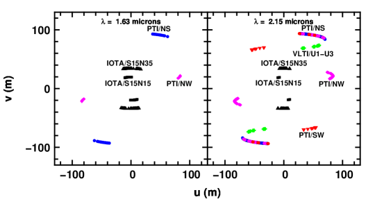
Figure 1: (u,v) tracks corresponding to the observations of FU Orionis. Left panel: H data; right panel: K data. The $(u,v)$ points have been labeled with the interferometer and the baseline used.

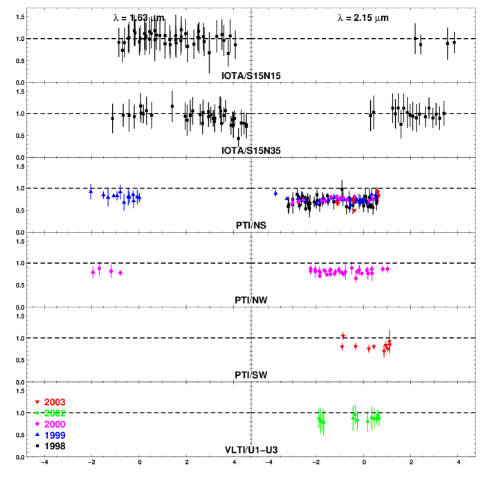
Figure 2: Calibrated squared visibilities of FU Orionis as function of hour angle in H (left column) and K band (right column). Rows from top to bottom display data obtained with the 6 interferometric baselines.

The observations with all interferometers covered a range of hour angles large enough to allow the projected baselines on the sky to rotate over a significant angle. Figure 1 displays the resulting $(u,v)$ plane coverage of our observations with the six baselines: 21m (IOTA-S15N15), 38m (IOTA-S15N35), 85m (PTI-NW), 87m (PTI-SW), 100m (VLTI-U1U3) and 110m (PTI-NS).

Figure 2 shows our results for the six baselines in the H and K bands (left and right columns respectively). All panels show calibrated squared visibilities as a function of hour angle. The main raw results are:

• We confirm the 1997 result (paper I): FU Orionis is resolved at 110m in the K band with the same visibility range (PTI-NS data) of $0.72\pm 0.07$ (cf. paper I).

• FU Orionis is also resolved at about the same visibility level with the 85m PTI-NW, 87m PTI-SW, and 100m VLTI-U1-U3 baselines.

• FU Orionis is unresolved at short baselines (IOTA data).

• We obtain color information between $1.6\mu\text{m}$ (H-band) and $2.15\mu\text{m}$ (K-band).

• We detect a peak-to-peak oscillation of 10% at 110m in the K band and more marginally in the H band (this oscillation appears better in binned data of PTI/NS displayed in the right panel of Fig. 4).

5 Interpretation of FU Ori observations

Interpretation of the observations performed with infrared long-baseline interferometers is not obvious since we have no direct information about the brightness distribution of the object. However, the measured visibilities allow us to set constraints on current models. In paper I, we had only one visibility point at 110m. However, thanks to the spectral energy distribution of FU Ori, we concluded that the data were compatible with a standard accretion disk model. The binary scenario was also compatible with the data, but still required an accretion disk to explain the SED.

We see here in the data the conjunction of 2 phenomena: a global decrease of the visibility with baseline and an oscillation as function of the spatial frequency. This can be explained by:

• the presence of a source which is marginally resolved and which dominates the overall flux,

• and by the presence of a second, fainter source. The fainter source can produce the oscillatory feature if it is located at a distance larger than the typical size of the compact centered structure.

The total complex visibility which results from these two objects is composed of the addition of the two terms (see Boden 2000, for the mathematical details).

5.1 Small-scale and bright structure

In this section we focus our attention on the visibility behavior without considering the oscillations. Though we perform the model fits with all individual measurements, for clarity we plot the results with baseline-averaged visibilities, as displayed in Table 3.

Table 3: Averaged square visibilities for the 6 baselines.

baseline	$\lambda$	$B_{\text{p}}$ (m)	$\theta$ (deg)	$|V^{2}|$
IOTA/S15N15	H	$20.2\pm 0.5$	$104.5\pm 9.5$	$1.00\pm 0.13$
IOTA/S15N35	H	$35.0\pm 0.7$	$95.7\pm 13.7$	$0.91\pm 0.14$
PTI/NS	H	$103.7\pm 2.2$	$61.8\pm 3.5$	$0.83\pm 0.04$
PTI/NW	H	$85.6\pm 1.5$	$14.1\pm 0.8$	$0.79\pm 0.05$
IOTA/S15N15	K	$20.8\pm 0.3$	$114.9\pm 3.4$	$0.90\pm 0.13$
IOTA/S15N35	K	$34.4\pm 0.3$	$91.4\pm 7.8$	$0.98\pm 0.09$
PTI/NS	K	$102.7\pm 3.8$	$63.6\pm 6.5$	$0.72\pm 0.08$
PTI/NW	K	$84.2\pm 1.8$	$14.0\pm 1.8$	$0.79\pm 0.05$
PTI/SW	K	$82.5\pm 2.9$	$-55.6\pm 4.9$	$0.82\pm 0.08$
VLTI/U1-U3	K	$89.6\pm 7.2$	$54.2\pm 5.3$	$0.87\pm 0.05$

5.1.1 Fitting strategy

We use a disk model and a methodology similar to those of paper I, but the data and technique used have undergone several changes: the method to compute visibilities is now based on Hankel transforms, valid for axisymmetric distributions (See Eq. 3); in the disk model the exponent of the temperature profile power-law is a free parameter, allowing us to describe flared irradiated disks as well as self-heated viscous ones; visibility data taken with all baselines are included in the study; the SED now comprises observations of the Gezari et al. (1999, 5th edition) catalog and from the 2MASS survey (Cutri et al. 2003). This model, although very simple, is able to reproduce a variety of situations without introducing new free parameters.

The model consists of a geometrically flat and optically thick disk with an inner radius $r_{\text{min}}$ and outer radius $r_{\text{max}}$, and features a radial temperature profile given by

$$T(r)=T_{0}\left(\frac{r}{r_{0}}\right)^{-q},$$ (1)

where $r_{0}=1$ AU is the reference radius, $T_{0}$ the effective temperature at $r_{0}$, and $q$ a parameter usually ranging from $0.50$ (flared irradiated disks) to $0.75$ (standard viscous disks or flat irradiated disks). Each part of the surface of the disk located at radius $r$ is assumed to emit as a blackbody at temperature $T(r)$, so that the flux and visibility are deduced by radial integration for a face-on disk with an inclination angle $i=0$:

$$F_{\lambda}(0) =\frac{2\pi}{d^{2}}\int_{r_{\text{min}}}^{r_{\text{max}}}rB_{\lambda}[T(r)]\,\text{d}r$$ (2)

$$V_{\lambda}(B_{\text{p}},0) =\frac{1}{F_{\lambda}(0)}\frac{2\pi}{d^{2}}\int_{r_{\text{min}}}^{r_{\text{max}}}rB_{\lambda}[T(r)]J_{0}\left[\frac{2\pi}{\lambda}B_{\text{p}}\frac{r}{d}\right]\,\text{d}r$$ (3)

with $J_{0}$ the zeroth-order Bessel function of the first kind, $B_{\lambda}$ the Planck function, $d$ the distance of the system and $B_{\text{p}}$ a projected baseline. For a disk presenting an inclination $i$ and a position angle $\theta$, these quantities become

$$F_{\lambda}(i) =F_{\lambda}(0)\cos i,$$ (4)

$$V_{\lambda}(\mathbf{B}_{\text{p}},i) =V_{\lambda}\left(B_{\text{p}}(i,\theta),0\right),$$ (5)

where the corresponding baseline is

$$B_{\text{p}}(i,\theta) =\sqrt{B_{u,\theta}^{2}+B_{v,\theta}^{2}\cos^{2}i}$$ (6)

and the coordinates are expressed in the reference frame rotated by the angle $$\theta$$,

$$B_{u,\theta} =B_{u}\,\cos\theta-B_{v}\,\sin\theta$$ (7)

$$B_{v,\theta} =B_{u}\,\sin\theta+B_{v}\,\cos\theta.$$ (8)

The companion, FU Ori S, observed by Wang et al. (2004) and the contribution of the FU Ori central stellar source have negligible and compensating effects on the measured visibilities. FU Ori S is located $0.5\,\text{arcsec}$ away from the bright object, far outside the interferometric field of view (viz. the “delay beam”, $\theta_{d}=\frac{\lambda^{2}}{\Delta\lambda B}\sim 0.1\,\text{arcsec}$), and will therefore only combine incoherently with the flux from FU Ori N. The bias introduced by this incoherent flux corresponds to the contribution of this companion flux to the total, i.e. 1.6% decrease in visibility. In addition, we neglect the contribution of the central star, since it is unresolved and will only slightly increase the visibilities. The contribution is of the order of 2%, almost cancelling the decrease of visibility due to FU Ori S.

5.1.2 Best fit and parameter constraints

Table 4: Model parameters for the small-scale structure. This best fit has a reduced $\chi^{2}$ of 1.16 (with 306 individual measurements) and a “goodness of fit” of 2%. The 3-$\sigma$ uncertainties on each parameter have been determined from a $\chi^{2}$ map around the minimum, as shown in left part of Fig. 5.

Accretion disc
$r_{\text{min}}$	$5.5_{-1.8}^{+2.9}$ $R_{\odot}$	$r_{\text{max}}$	$100$ AU (fixed)
$T_{0}$	$745_{-24}^{+24}$ K	$q$	$0.71_{-0.04}^{+0.05}$
$i$	$55_{-7}^{+5}\,\text{deg}$	$\theta$	$47_{-11}^{\hphantom{0}+7}\,\text{deg}$

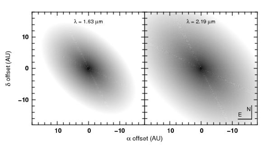
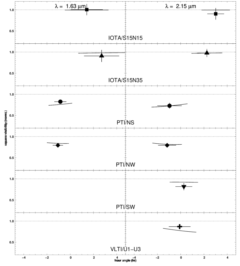
Figure 3: Accretion disk model with baseline-averaged data corresponding to parameters listed in Table 4. Lines correspond to the model and symbols to measurements. The dotted line corresponds to an unresolved object. For the sake of clarity, data have been binned in the figure, but the model fit was performed using individual measurements. Top-left panel: spectral energy distribution and best fit model. Right panel: visibility data versus hour angle in H and K. Bottom-left panel: synthetic images in H and K in logarithmic scale. East is left and North is up.

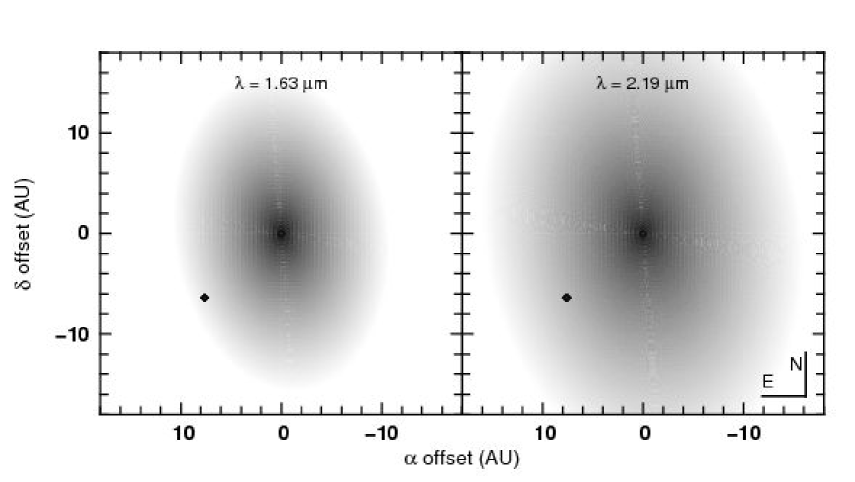
Figure 4: Disk-spot model corresponding to parameters of Table 5. Lines corresponds to the best model fit and markers to visibilities from Fig. 2 in binned form. Top-left panel: spectral energy distribution and best fit model. The solid line stands for the whole model and the dashed one for the spot. Right panel: visibility data vs. hour angle for each baseline in H and K. The contribution of the disk is displayed in dashed lines. Bottom-left panel: synthetic image in logarithmic scale. East is left and North is up.

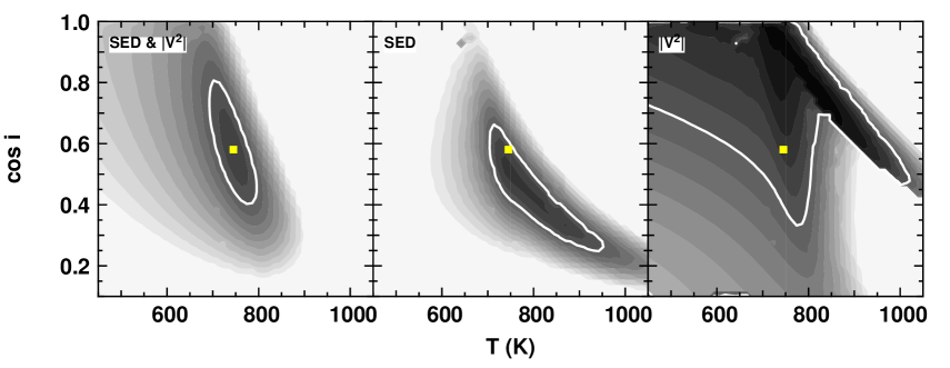
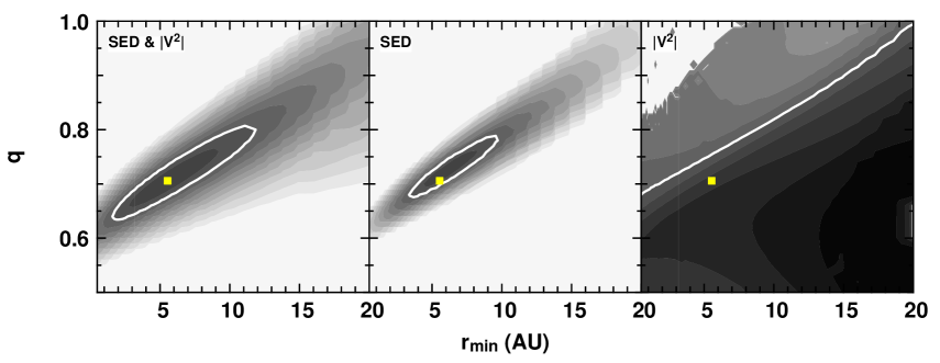
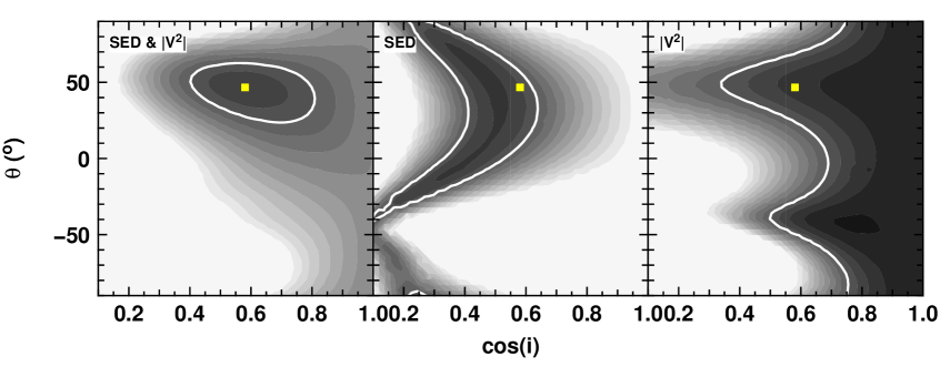
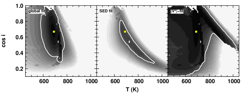
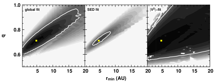
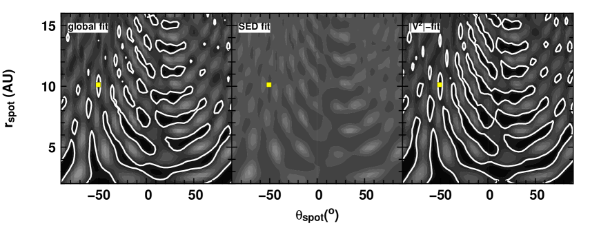
Figure 5: $\chi^{2}$ distribution of the disk alone (left column) and disk-spot (right column) models around the best fit (marked with a square). The white solid line draws the 3-$\sigma$ limit (“goodness-of-fit” $>0.25$%). Top: inclination vs. temperature. Middle: temperature law exponent vs. minimum radius. Bottom left: inclination vs. position angle of the disk. Bottom right: position angle of the spot vs. projected distance to the centre. Left subpanels: $\chi^{2}$ determined with both visibility and SED data. Middle subpanels: $\chi^{2}$ determined with the SED only. right subpanel: $\chi^{2}$ determined with the visibilities only.

When trying to interpret the measured visibilities and the SED for the small-scale structure with the previous simple disk model (neglecting the spot), the best fit has been unambiguously found using a $\chi^{2}$-gradient search method. The reduced $\chi^{2}$ is 1.16, and the probability that statistical deviation from the model results in as large a deviation is 2% (“goodness of fit”). This implies that the model is unlikely to explain the observations (since we have been quite conservative in our determination of the data uncertainty), but we cannot rule out this possibility. This low goodness gives credence to trying the more complicated model with a spot (see Sect. 5.2). The parameters obtained are presented in Table 4, with the standard uncertainty on the parameters. These errors have been determined from the $\chi^{2}$ distribution displayed in left part of Fig. 5 — assuming a Gaussian error distribution. We checked that the uncertainties derived have values close to those predicted from the quadratic estimate of the $\chi^{2}$ near its minimum.

Unlike interferometric observations of T Tauri and Herbig Ae stars (Millan-Gabet et al. 1999; Akeson et al. 2000, 2002; Eisner et al. 2003, 2004), the visibilities for FU Ori are compatible with the simple power-law radial temperature profile predicted by the standard disk model. We derive a temperature exponent $q\approx 0.71\pm 0.05$, which is actually strongly constrained by the slope of near-IR SED, and fairly consistent with the visibilities. The derived high temperature of about $745\pm 24\mbox{ K}$ at 1 AU hints to a viscous, self-heated disk rather than an irradiated disk.

The shape of the visible SED sets a constraint on the cut-off radius $r_{\text{min}}\approx 3$–$8\,R_{\odot}$. We find that the intensity of the near-IR emission strongly determines $T_{0}\cos i$, while individual constraints on $T_{0}$ and $i$ are provided by the visibilities. The latter indeed determine $T_{0}$, $r_{\text{min}}$, $i$ and $\theta$ (they have an influence resp. on the spatial extent of the disk in H and K, on the amount of central unresolved flux, and on the spatial extent in a particular direction), but their impacts are coupled. However, the visibilities also constrain the radial brightness distribution, provided that they be taken across a range of wavelengths, as explained by Malbet & Berger (2002); Lachaume (2003). The visibilities at different baseline orientations constrain the inclination and the position angle of the disk. The visibilities at short baselines put no constraints on the geometry of the disk because it is only marginally resolved (Lachaume 2003), but we can rule out the contribution of an extended (sub-arcsec) structure (e.g. scattering by an envelope) because IOTA visibilities at $B_{\text{p}}\lesssim 30$ m are unresolved.

Figure 3 illustrates the comparison between the model and the observations. The SED data and the result of the fit are displayed in the upper left panel. The visibilities averaged by baseline, listed in Table 3, are presented in the right panel with the visibility curves corresponding to the $(u,v)$ track of each baseline. Finally in the lower left panel, we show the corresponding synthetic image of the disk.

5.2 Large-scale structure

In this section we focus our attention on the high-frequency oscillation in the visibility function, mostly visible in the 110m $K$-band data of PTI. We believe it to come from an off-center unresolved light source that we call a “spot”. We fit to the data a compound source model consisting of an accretion disk (as described above) and an unresolved spot. The latter is modeled as a circular black-body of uniform brightness with a temperature $T_{\mathrm{spot}}$ and a radius $r_{\mathrm{spot}}$. The two components are separated by the projected physical distance $d_{\mathrm{spot}}$ with a position angle $\theta_{\mathrm{spot}}$ (with a $180\,\text{deg}$ ambiguity). The fitting procedure is the same as in Sect. 5.1.

5.2.1 Properties of the spot

Table 5: Model parameters for the large-scale structure without secular variation. The reduced $\chi^{2}$ of the best fit is 0.95 (with 306 individual measurements) and the “goodness of fit” is 70%.

Binary system
$d_{\mathrm{spot}}$ a	$10.1_{-0.3}^{+0.4}$ AU	$\theta_{\mathrm{spot}}$ a	$-50_{-1}^{+1}\,\text{deg}$
Accretion disc
$r_{\text{min}}$	$4.9_{-3.7}^{+2.8}$ $R_{\odot}$	$r_{\text{max}}$	$100$ AU (fixed)
$T_{0}$	$692_{-41}^{+29}$ K	$q$	$0.71_{-0.04}^{+0.08}$
$i$	$48_{-10}^{\hphantom{0}+9}\,\text{deg}$	$\theta$b	$8_{-21}^{+21}\,\text{deg}$
Uniform stellar disc
$T_{\mathrm{spot}}$b	$4600_{-800}^{+800}$ K	$r_{\mathrm{spot}}$	$5.0\ R_{\odot}$ (fixed)
a Other distant minima exist.
b Quadratic error from the fitting routine

The best model fit was obtained with the parameters listed in Table 5. The reduced $\chi^{2}$ is 0.95 and the probability that statistical deviation from the model accounts for as large a deviation is 70%, so the fit appears as a consistent explanation for the data – in comparison to the 2% of the disk-alone model – but the detection of the structure is only at a 2-$\sigma$ level. The best-model fit is shown in Fig. 4, and the probability distribution around the minimum is shown in the right part of Fig. 5.

The disk parameters and their uncertainties are consistent with the results of Sect. 5.1 except for the position angle: its uncertainty is much larger in our last model fit ($8\pm 20\,\text{deg}$) than in the previous one ($47\pm 10\,\text{deg}$), and both values differ by $2\sigma$. This angle is constrained (together with the inclination) by the visibility difference at three different baseline angles, namely with the NW, SW, and NS PTI baselines (see the right panel of Fig. 4). When a spot is added, this difference is changed, resulting in a different position angle: in our best fit, the disk visibility for the NS baseline is unchanged since it is the average of the oscillations, while it is higher for the NW and SW baselines because the measured visibility (disk plus spot) is in the low of the oscillations.

As Fig. 5 shows (see bottom panel, $\chi^{2}$ as a function of the spot location), there are multiple acceptable “best” model fits featuring radically different spot locations. The aforementioned solution is actually the best in terms of modelling the PTI/NW and NS oscillation in K, but was not found to be statistically better than others that do not feature such oscillation. We think, however, that the oscillation is actual and that the model ambiguity results from the poor accuracy of other measurements (IOTA in H and K, and PTI in H). Thus, results on the spot location should be taken with caution.

We have chosen to parametrize the flux of this spot in terms of stellar photosphere with the temperature and the radius of the photosphere as parameters. However only the $K$ data can be used to constrain them and we have fixed the value of the radius to $5R_{\odot}$, which is typical for a young star. The derived temperature depends strongly on the value taken for the radius and therefore should be considered with caution.

The location of the spot is quite well constrained by the shape of the oscillation with a projected distance to the center of $10\pm 1$ AU and a position angle $-50\pm 1\,\text{deg}$ (with 180 deg ambiguity). The amplitude of the oscillations in the K-band constrains the flux ratio of the spot to the primary, $\Delta K\approx 3.9\pm 0.2$ and $\Delta H\approx 3.6\pm 0.2$ mag. However, there are other acceptable $\chi^{2}$ minima (goodness-of-fit $\gtrsim 50$%, see the bottom right $\chi^{2}$ maps in Fig. 5) which do not reproduce the oscillation, but they cannot be ruled out. We should note that the oscillations are detected mostly in the $K$ band and therefore $\Delta H$ is not constrained by both the oscillations and the model, since there is little chance that a spot at $4000-5000\,\text{K}$ be a pure black-body.

5.2.2 Secular evolution

Assuming that the spot location of the disk-spot model is that derived in Sect. 5.2.1 (which allows us to explain the PTI oscillation in K), we carried out a model fit of its location for each year of observation. The results are displayed in Table 6. The fit is successful in the years 1998, 1999, and 2000 and feature a 3-$\sigma$ detection of an almost radial motion. The data obtained in 2003 are not sufficient to constrain the position of the spot for this year explaining the bad $\chi^{2}$.

Table 6: Parameters of the best model fit of the location of the spot in 1998, 1999, 2000, and 2003, and its quality.

year	$d_{\mathrm{spot}}$ (AU)	$\theta_{\mathrm{spot}}$ (deg)	$\chi^{2}$ (total)	$\chi^{2}$ ($|V|^{2}$)
1998	$8.0\pm 1.9$	$-48.0\pm 3.3$	0.63	0.54
1999	$9.6\pm 1.5$	$-49.4\pm 2.2$	0.95	0.78
2000	$10.1\pm 0.6$	$-50.3\pm 1.6$	1.04	0.91
2003	$11.1\pm 0.3$	$-49.9\pm 1.7$	2.54	4.02

6 Discussion

6.1 Accretion disk versus photosphere

The current data set confirms the result from paper I and shows consistent visibility data. We can definitively confirm that we are observing an object whose size (Gaussian full width at half maximum) is 1.5mas in $K$ wide corresponding to 0.7AU or $150R_{\odot}$ at a distance of 450 pc (see paper I for details). Therefore if Herbig et al. (2003) is correct in interpreting the high resolution spectroscopic data as stellar chromospheric activity, then the star must be accompanied by cooler circumstellar material that spreads beyond $150R_{\odot}$ that is probably a circumstellar disk.

The temperature $T_{0}$ obtained in our fits yield an accretion rate of $\dot{M}=(6.3\pm 0.6)\times 10^{-5}(M_{\star}/M_{\odot})^{-1}\,M_{\odot}/\text{yr}$ for the disk alone and of $\dot{M}=(4.7\pm 0.6)\times 10^{-5}(M_{\star}/M_{\odot})^{-1}\,M_{\odot}/\text{yr}$ for the disk accompanied by a spot. The effective temperature-accretion rate relation is the one of the standard model (see Eq. 2.7 in Shakura & Sunyaev 1973). It is interesting to note that the corresponding temperature at the inner radius is 10050 K (resp. 10140 K). In our present model, the disk is optically thick whatever the physical process which dominates the opacity (gas or dust). A more detailed study of this boundary region would be of great interest.

Compared to paper I, we are able to begin constraining the geometry of the accretion disk, with an inclination angle of the order of 50 degrees and position angle of the order 10–40 degrees. More accurate data and better $(u,v)$ coverage is still desirable, but we already show the path toward such constraints.

Other observations of Herbig Ae stars (Millan-Gabet et al. 2001; Akeson et al. 2002; Eisner et al. 2003, 2004) and of T Tauri stars (Akeson et al. 2003; Colavita et al. 2003) cannot be interpreted in the framework of the standard disk model. Measured near-IR visibilities are smaller than the theoretically expected values, suggesting puffed-up inner disk walls, and flaring is often necessary to fit mid- and far-IR photometry (Dullemond et al. 2001; Muzerolle et al. 2003). In contrast, our work on FU Ori, as well as some Herbig Be stars observed by Eisner et al. (2004), shows that the observed circumstellar disk structure is consistent with the standard accretion disk model, i.e. geometrically flat and optically thick with a temperature law index close to 0.75. We suggest that accretion-dominated objects (such as FUors and Herbig Be stars) fit the standard accretion disk model, while Herbig Ae stars and T Tauris may have different disk structures due to the influence of irradiation. This is also consistent with the fact that in FUors the disk completely dominates the luminosity and therefore the physics of the disk would be expected to be governed by accretion and not by external stellar heating.

Hartmann & Kenyon (1985) have presented an interesting interpretation of double lines observed in FU Ori by spectroscopy. The controversy with Herbig et al. (2003) comes from the fact that these authors are not able to localize the origin of these lines. The explanation of Hartmann & Kenyon (1985) appears to be more consistent with our data.

The interferometric instrument AMBER on the VLTI (Petrov et al. 2001) has the potential to detect these double lines and identify the region where they are emitted (Malbet et al. 2003).

6.2 The nature of the bright spot

Our analysis of the data shows that the scenario which involves a bright spot is more likely to explain our observations. The presence of such a spot would modulate the visibility curves. Even if the amplitude of the oscillations is not large and the number of cycles is small, we believe that this spot is indeed present. As can be seen in Fig. 4, the ripples of the visibility also explain some low visibilities obtained at IOTA with short baselines. This detection was already pointed out by Berger et al. (2000), based on a smaller data set, and the latest observations confirm this behavior. In addition, our analysis by year, using independent sets of observations, yields parameters which are close to each other. To confirm the presence of this bright spot, we suggest observing FU Orionis in several wavelengths and possibly with spectroscopy (see Fig. 6 for an example of the correlated spectrum that would be obtained with a specific configuration of the VLTI with the instruments AMBER and MIDI).

The nature of this bright spot is still unknown. This structure, assuming it is unresolved, could be due to an increase of the intensity in the disk due to a thermal outburst (Clarke et al. 1990; Bell & Lin 1994; Bell 1999). If the assumption of a photosphere radius of $5R_{\odot}$ is correct (see remark in Sect. 5.2.1), the derived color temperature of $4600\,\text{K}$ of this spot is similar to temperatures observed in stellar photospheres and therefore is consistent with the presence of a young stellar companion.

The year-by-year analysis indicates that the spot may be moving with a velocity of about $1.2\pm 0.6\,\text{AU}\cdot\text{yr}^{-1}$ on a rectilinear trajectory. We have insufficient data to complete the analysis but additional data will provide more time-sampling to confirm or exclude the motion of the spot. The proper motion of FU Ori is $116\pm 104\times 10^{-5}\,{\rm s/yr}$ in right ascension and $86.4\pm 15.5\,{\rm mas/yr}$ in declination (Carlsberg Meridian Catalogue: Copenhagen University Observatory et al. (1999)), i.e. $39\pm 7\,\text{AU}/\text{yr}$ at position angle of $12\pm 10\,\text{deg}$. The spot motion, if actual, is therefore not due to a foreground or background star. It could be explained by the motion of a companion star orbiting on a very highly eccentric orbit around the primary star or an orbit inclined with respect to the disk.

This explanation is consistent with the scenario introduced by Bonnell & Bastien (1992) and recently revisited by Reipurth & Aspin (2004b) following the discovery of a binary companion to FU Ori (Wang et al. 2004). The companion observed by Wang et al. (2004) cannot be responsible for, or be the consequence of, the 1936 outburst as noted by Reipurth & Aspin (2004b). However these same authors have also pointed out that “FU Orionis itself must be a close binary, with a semi-major axis of $10\,\text{AU}$ or less”. Confirmation and extension by future measurements are needed to confirm that the spot we are observing might indeed be the companion they were looking for located on an inclined or highly eccentric orbit.

This spot could also represent the signature of the presence of a young planet. Recently (Lodato & Clarke 2004) proposed that FUor outbursts could be caused by a planet at about 10$R_{\odot}$ which causes gap instabilities. In the case of FU Ori, the mass of the planet would have had to be $\sim 15M_{\rm Jupiter}$ in order to explain the rapid rise of the luminosity up to $500L_{\odot}$. We do not have enough color measurements to derive the temperature and the luminosity of the spot in order to check that it is compatible with a $15M_{\rm Jupiter}$ planet. Nor can we explain why the planet would be migrating away from the center.

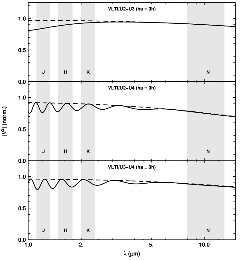
Figure 6: Predicted squared visibility curve of the disk+spot model for FU Ori through the infrared spectrum with the triplet of VLTI 8m telescopes U2-U3-U4.

7 Conclusion

We have presented the most complete set of interferometric observations obtained so far in the domain of star formation with several infrared interferometers: PTI, IOTA and VLTI. These observations help us to better understand the exact nature of FU Orionis. Our measurements confirm that FU Ori hosts an active accretion disk with a $\approx 5\times 10^{-5}M_{\odot}/\text{yr}$ accretion rate. We have also marginally detected an unresolved bright structure, that we identify as a possible close companion on a highly eccentric orbit. This putative companion may be responsible for the outburst of the accretion rate that led to the rapid increase of the luminosity.

These observations also show that the inner structure of YSOs is rather complex and cannot be fully understood with only a small number of interferometric observations. More wavelength and $(u,v)$ coverage is required to fully constrain models. The next step will probably be the reconstruction of an image of this interesting object based on extensive observations with the VLTI.