A Model for Multidimensional Delayed Detonations in SN Ia Explosions

We show that a flame tracking/capturing scheme originally developed for deflagration fronts can be used to model thermonuclear detonations in multidimensional explosion simulations of type Ia supernovae. After testing the accuracy of the front model, we present a set of two-dimensional simulations of delayed detonations with a physically motivated off-center deflagration-detonation-transition point. Furthermore, we demonstrate the ability of the front model to reproduce the full range of possible interactions of the detonation with clumps of burned material. This feature is crucial for assessing the viability of the delayed detonation scenario.

tars: supernovae: general – Hydrodynamics – Methods: numerical

1 Introduction

The widely accepted standard model for type Ia supernovae (SNe Ia) is the thermonuclear explosion of a C+O white dwarf that has reached the Chandrasekhar mass by means of mass accretion from a binary companion (e.g. Hillebrandt & Niemeyer, 2000, and references therein). This scenario has recently received new support from the tentative discovery of the companion star of Tycho’s supernova by Ruiz-Lapuente et al. (2004).

While this idea has been around since the original work by Hoyle & Fowler (1960) and countless CPU cycles have been spent in search of a realistic model, some crucial aspects of the explosion physics are still not understood. Apart from the scientific challenge of reproducing the inner workings of these fascinating astronomical events of which we already know so many details (e.g. Matheson et al., 2004; Benetti et al., 2004), their potential as cosmological distance indicators has provided us with yet another strong motivation to construct predictive, self-consistent explosion models. Two subjects take center stage in most current debates: (i) the conditions under which the dynamical phase of the explosion ignites and (ii) the thermonuclear flame forms (Woosley et al., 2004), and the questions surrounding the possibility of a deflagration-detonation-transition (DDT) (Niemeyer & Woosley, 1997; Khokhlov et al., 1997) during the late phase of the explosion, giving rise to a “delayed detonation” (Woosley & Weaver, 1994; Khokhlov, 1991; Yamaoka et al., 1992). The modeling and consequences of the latter are the topics of this paper.

Detection of intermediate mass elements in the early spectra of SNe Ia is usually interpreted in terms of an initial phase of subsonic thermonuclear burning (deflagration) that allows the star to expand to lower densities. The thin deflagration front is hydrodynamically unstable, most importantly as a result of the Raleigh-Taylor (RT) instability, so it quickly becomes fully turbulent. Different models for the unresolved turbulent flame structure have been employed in multidimensional simulations of exploding white dwarfs (Niemeyer & Hillebrandt, 1995; Khokhlov, 1995; Reinecke et al., 1999a); however, the global properties of the explosion appear to be robust with respect to the particular choice of subgrid-scale model (Reinecke et al., 2002; Gamezo et al., 2003).

On the other hand, interpretations of the simulations with regard to whether or not a DDT must occur differ considerably. Pure deflagration models with the currently achievable grid resolution produce too little ⁵⁶Ni when compared with one-dimensional models that successfully fit the observational data. Moreover, they generically leave behind unburnt material near the stellar core, whose amount is strongly constrained by the lack of carbon features in late SN Ia spectra. It has been claimed that this is a problem intrinsic to all turbulent deflagration models which can only be solved by a delayed detonation that burns up all of the C+O left in clumps of varying sizes near the core (Gamezo et al., 2004).

Owing to the fine-tuning required to achieve a DDT in unconfined media (Niemeyer 1999; strengthened by the recent results of Bell et al. 2004) and to the promising trend in highly resolved turbulent deflagration models for burning progressively more material in the core (Niemeyer et al., 2003), we believe that the jury is still out on the question of delayed detonations. Nevertheless, we will demonstrate in this work that the level-set method that has been succuessfully employed to model deflagration fronts in SN Ia simulations (Reinecke et al., 1999b) can be modified in a straightforward way to represent unresolved detonations. Its main advantage is its complete control over the front velocity at each point, allowing us to mimic the interaction of the detonation with unresolved and resolved clumps of ashes in a realistic manner. One of our main conclusions is the sensitivity of the results with respect to the way these interactions are implemented, supporting our claim that an accurate detonation model is necessary.

In previous attempts to simulate delayed detonations in multiple dimensions (Arnett & Livne, 1994; Gamezo et al., 2004), the detonation front was unresolved and no model for the propagation speed was employed. While it is well-known that the velocity of planar detonations is robust with regard to numerical resolution, the same is not true in the presence of obstacles or clumps of ash (closely related are consequences of the cellular front structure, see Timmes et al. 2000). In fact, fully resolved calculations show that C+O detonations can hardly pass through burned material at all, whereas this behavior is easily hidden by coarse resolution (Maier, 2005). Here, our approach is to compare the two limiting cases of (i) a detonation that passes through burnt material as a pure shock wave at the speed of sound and re-ignites on the other side and (ii) one that stalls immediately when it hits a clump of ash and needs to wrap around it to reach the other side.

In all of our simulations, we let the code decide where and when the DDT should take place. The criterion for a DDT follows from the comparison of the thermal flame thickness with the Gibson length of the turbulent flame brush (Niemeyer & Woosley, 1997; Niemeyer & Kerstein, 1997). As expected, we find that all DDTs occur near the outermost parts of the turbulent deflagration front, generally taking place earlier in off-center ignition models than in centrally ignited ones. It follows immediately that in order to burn the clumps of C+O near the core the detonation needs to propagate back into the star, having to pass through a foam of fuel and ashes along the way. This is the reason why an accurate treatment of the detonation-clump interactions is indispensable.

In what follows we give a short description of the flame algorithm employed to model both the deflagration, as well as the detonation front. In Section 3, we discuss the results of a series of test calculations determining the suitability of our approach to represent supersonic burning fronts. In Section 4, we present our DDT model and discuss the results and implications of our numerical study. Concluding remarks are made in Section 4.1.

2 Level set deflagration and detonation model

The numerical code applied in this work is based on Reinecke’s version of PROMETHEUS as described in Reinecke et al. (1999a, b). In particular, we employ the level set capturing/tracking scheme (Sethian, 1996) used in these references for turbulent deflagration fronts to model an additional delayed detonation. In this approach, the thermonuclear burning front is associated with the zero level set of a linear distance function $G(\mbox{\boldmath$x$},t)$. It thus represents a $n-1$-dimensional moving hypersurface in an $n$-dimensional simulation. For a similar approach to model deflagrations and detonations, see Fedkiw et al. (1999).

The front propagation is given by the temporal evolution of $G$,

$$\frac{\partial G}{\partial t}=(\mathbf{v}_{\mathrm{u}}\cdot\mathbf{n}+s)|\nabla G|\,,$$ (1)

depending on the fluid motion $\mathbf{v}_{\mathrm{u}}$ of the unburnt state and the propagation speed $s$ relative to it. The choice of $s$ reflects the kind of combustion front, whether deflagration (subsonic) or detonation (supersonic), and is provided as an external parameter as described in the next paragraph. Details about the level set function and its implementation can be found in Reinecke et al. (1999b). For the modeling of both deflagration and detonation fronts we used the cell averaged fluid velocity $\mathbf{\bar{v}}$ instead of $\mathbf{v}_{\mathrm{u}}$. Owing to this so-called passive implementation, as opposed to the full implementation, cf. Smiljanowski et al. (1997); Reinecke et al. (1999b), the transition between fuel and ashes is smeared out over about three grid cells.

As in previous simulations (Reinecke et al., 1999a, 2002), the speed of the deflagration front is defined as the upper limit of the laminar and turbulent burning velocities in the respective grid cell, $s_{\rm def}=\mathrm{max}(s_{\mathrm{lam}},s_{\mathrm{tur}})$. Here, $s_{\mathrm{lam}}$ is a known function of composition, density, and temperature (Timmes & Woosley, 1992), while $s_{\mathrm{tur}}$ is calculated by an additional subgrid-scale model taking fluid dynamics into account on scales smaller than the computational grid size (Niemeyer & Hillebrandt, 1995). The detonation velocities, $s_{\rm det}$, are taken from Sharpe (1999) as a function of the unburned fuel density.

Behind the front all material is immediately transformed into the reaction products, whereas inside the mixed cells we determine the volume fraction occupied by the burnt material and adapt the mass fraction of ashes correspondingly. For densities $\rho>5.25\times 10^{7}\,\mathrm{g/cm^{3}}$, the fuel is converted into ${}^{56}\mathrm{Ni}$, releasing a fusion energy of $7.86\times 10^{17}\,\mathrm{erg/g}$. At lower densities, the burning process only produces intermediate mass elements represented in our simulations by ${}^{24}\mathrm{Mg}$ and an energy release of $4.18\times 10^{17}\,\mathrm{erg/g}$. Below $\rho=10^{7}\,\mathrm{g/cm^{3}}$, no change of composition takes place.

3 Detonation test calculations

Since the front algorithm had so far only been applied for modeling deflagrations, its suitability for describing detonations had to be verified. Several one- and two-dimensional test calculations were carried out to investigate the influence of external factors like fuel density, grid resolution and time step on the front propagation.

In all simulations, the unburnt material was characterized by a uniform composition with equal mass fractions of ${}^{12}\mathrm{C}$ and ${}^{16}\mathrm{O}$ and an initial temperature of $T=10^{8}\,\mathrm{K}$. Unless otherwise stated, all fronts were set to propagate in a positive $x$-direction (and a positive $y$-direction in the 2D case) on a Cartesian grid with a cell size of $\Delta=10^{6}\,\mathrm{cm}$.

3.1 One-dimensional fronts

Figure 1: Temperature, density, fluid velocity, and chemical composition of a planar detonation front after 0.1 s. The spike in the density profile behind the shock is the result of a small numerical oscillation.

We investigated planar fronts propagating on a $200\times 4$ grid with reflecting boundaries at the left, top, and bottom edges of the computational domain and an outflow boundary to the right. Figure 1 shows the profiles of temperature, density, fluid velocity, and chemical composition of a detonation front 0.1 s after its initialization.

In order to investigate the ability of the front model to reproduce a given propagation velocity $s_{\rm det}$, we compared the time dependent $x$-positions of the detonation front with its theoretically predicted behavior for three different initial densities $\rho=10^{7},10^{8}$, and $10^{9}\,\mathrm{g/cm^{3}}$. To determine the position of the front, the values of the level set function in the direct neighborhood of the front were interpolated.

Additionally, to verify the obtained $x$-values, we directly calculated the propagation velocity $\tilde{s}_{\rm det}$ by averaging the mass fraction of ashes per cell over all 200 grid zones in the $x$-direction in every time step, multiplying with the physical grid length and dividing by time:

$$\tilde{s}_{\rm det}=200\,X_{\mathrm{ash}}(t)\frac{\Delta}{t}\,.$$ (2)

Here, $X_{\mathrm{ash}}(t)$ denotes the averaged time dependent mass fraction of ashes. Both methods gave virtually identical results. For all three densities, the measured numerical velocity of the detonation front $s_{\rm det}$ exceeded the provided one, $\tilde{s}_{\rm det}$, by approximately 10 %. As shown by further numerical tests, this behavior is affected neither by a change of the grid resolution nor by a considerable refinement of the time step, so that the error can be attributed to the inaccuracies in the passive implementation of the front model.

Reconsidering the velocity profile in Fig. 1, the reason for the excessive propagation speed becomes clear. In our simulation, the fuel is at rest, while the ashes behind the front proceed with $v_{\mathrm{b}}\approx 2\times 10^{8}$ cm s^-1. Averaging the two velocities results in a non-zero fluid velocity and therefore causes an error in Eq. 1 when replacing $\mathbf{v}_{\mathrm{u}}$ by $\mathbf{\bar{v}}$.

Since in these numerical tests the fuel had initially been at rest, the results shown above are only valid in the frame of reference of a non-moving gas. In order to test for a possible grid dependence of the front propagation scheme, the system of detonation front and gas was Galilei-transformed in a further simulation. Here, the C+O gas flowed uniformly in the negative $x$-direction with a velocity $v_{x}=-1.16\times 10^{9}$ cm s^-1, and the reflecting boundary condition at $x=0$ was changed to outflow. The front was ignited at the center of the grid. Since $|v_{x}|$ was chosen to be equal to $s_{\rm det}$ at the density $\rho=10^{8}$ g cm^-3, the front should remain at rest in the grid frame on its right hand side while propagating with double velocity to the left.

Figure 2: Detonation profile $0.018\,\mathrm{s}$ after initialization in a C+O gas of velocity $v_{x}=-1.16\times 10^{9}$ cm s^-1.

The profile of the front $0.018\,\mathrm{s}$ after its initialization can be seen in Fig. 2. The measured deviation ($\approx 7$ %) is equal in both directions, showing that the front model is insensitive to Galilei transformations. This fact allows a simple correction of $s_{\rm det}$ to account for the numerical error.

3.2 Two-dimensional fronts

For the investigation of fronts in two dimensions, the grid was expanded from 4 to 200 cells in the $y$-direction. Calculations with circular detonations showed that the front kept its shape throughout the simulation time, differing insignificantly from the exact circle geometry (Fig. 3). As in the case of planar detonations, the small deviations of the front velocity from its theoretical value can be explained by the fact that the front is not advected with the speed of the unburnt matter in Eq. (1) but by the average speed in the burning cells.

Comparing our findings to the results of Reinecke et al. (1999b), one can see that the front algorithm causes errors like those for both kinds of burning fronts, with the difference that the speed is too low in the case of deflagrations while being too high in the case of detonations. The reason for this opposite behavior is that in the earlier work, all material behind the front is at rest while the fuel expands at high velocities. Underestimation of the propagation speed is therefore a consequence of averaging the fluid velocities in the cells cut by the front. In contrast to our previous expectations, the higher density jump across the front does not result in a larger inaccuracy for detonations.

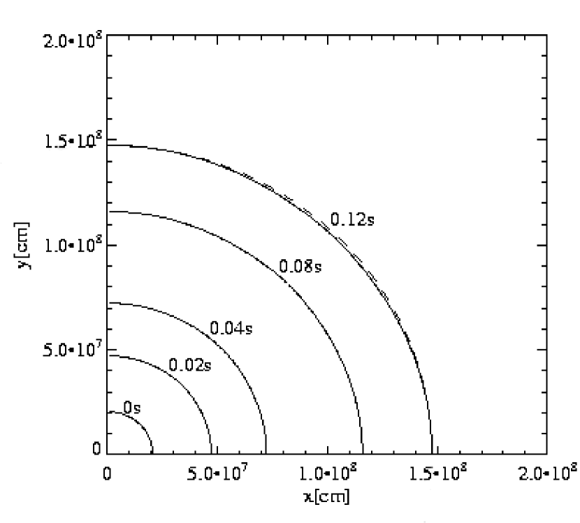
Figure 3: Front geometry of a centrally initialized circular front propagating outwards. The dashed line represents an exact circle.

4 Two-dimensional simulations of delayed detonations

The supernova simulations were carried out in cylindrical coordinates on a Cartesian grid in the $r$-$z$-plane. The center of the white dwarf was placed into the origin of a $256\times 256$ mesh with equally spaced cells of a side width $\Delta=10^{6}\,\mathrm{cm}$. Thus, we modeled one quadrant of the star, assuming mirror symmetry along the $r=0$ and $z=0$ axes. To take the expansion of the star into account during the explosion and to avoid violating of mass conservation due to an outflow of stellar material over the grid borders, the size of the outermost grid zones grew exponentially beginning with the 222nd zone.

The white dwarf, constructed in hydrostatic equilibrium for a realistic equation of state, had a central density of $2\times 10^{9}$ g cm^-3, a radius of about $1.9\times 10^{8}\,\mathrm{cm}$, and a mass of $2.8\times 10^{33}\,\mathrm{g}$. The initial mass fractions of C and O were chosen to be $X_{\mathrm{C,O}}=0.5$, and the total binding energy turned out to be $-5.2\times 10^{50}\,\mathrm{erg}$.

The deflagration phase of the models Z1, Z3, B1, and B5 was initialized and evolved identically to Reinecke et al. (1999a). For modeling the delayed detonation, a second level set function (LSet2) was implemented in addition to the first one (LSet1) describing the deflagration front. In order not to disturb the flame propagation during the deflagration phase, the value of LSet2 was set to a negative value.

A DDT was assumed to occur as soon as the transition from flamelet to distributed burning regime took place for the first time during the explosion (Niemeyer & Woosley, 1997; Niemeyer & Kerstein, 1997). In order to identify the corresponding time and grid location, the thermal flame width $\delta$ was compared to the Gibson length, defined by $l_{\mathrm{Gibs}}=\Delta\left(s^{2}_{\mathrm{lam}}/2q\right)^{3/2}$, in each time step. The values of the flame width as a function of density were taken from Timmes & Woosley (1992). A detonation was initialized as a circular front with a radius of $10^{6}\,\mathrm{cm}$ at the point where the condition $l_{\mathrm{Gibs}}=\delta$ was first satisfied.

So far, the question whether a thermonuclear detonation front can propagate through burnt stellar material has not received much attention. It is conceivable that the pressure wave is strong enough to ignite the carbon again when it re-enters a region of fuel. However, fully resolved simulations suggest that this is not the case even for relatively small clumps of ash (Maier, 2005). Depending on the behavior of the detonation front, isolated bubbles of fuel may be left inside the stellar core even after a delayed detonation has taken place, in disagreement with spectral observations in the nebular phase.

In order to test the capability of our detonation model to cover the whole range of expected front behavior, we investigated the limiting cases of a detonation that first crosses the burnt material as a shock wave with sound velocity and then re-ignites on the other side (Case a), and a detonation that dies immediately upon running into ashes (Case b). The latter was modeled by setting $s_{\rm det}=0$ in burnt regions.

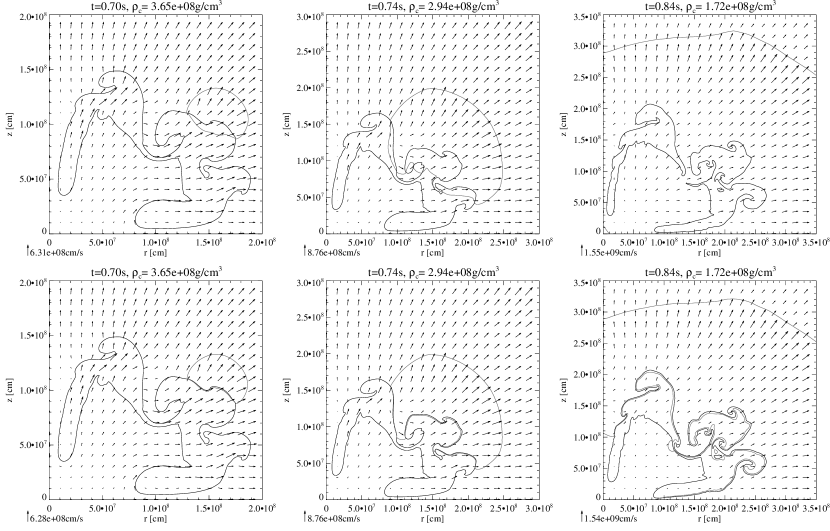
Figure 4: Temporal evolution of the front geometry and velocity field for the Models B1a (top row) and B1b (bottom row). The snapshots were taken at equal times. The convoluted front corresponds to the initial deflagration, and the smooth curve that grows with time depicts the detonation front.

The time evolution of the front geometry and flow field in the non-central one-bubble model B1 is shown in Fig. 4 where we compare three snapshots of the explosion scenarios a and b at $t=0.7\,\mathrm{s}$, $0.74\,\mathrm{s}$ and $0.84\,\mathrm{s}$. As an additional measure for the expansion of the star, the central density is noted in every plot. By construction the deflagration phase is identical for both Cases a and b.

After the DDT which takes place at $t=0.68\,\mathrm{s}$ at a distance $r\approx 1.5\times 10^{8}\,\mathrm{cm}$, the differences between Models B1a and B1b become visible. The detonation in Model B1b cannot cross the bubble of burnt material until the latter breaks apart at its thinnest point at $t\approx 0.84$ s (lower right plot of Fig. 4). Notice that the breaking is only a numerical artifact since burnt regions cannot disconnect in the absence of flame quenching; more realistic, i.e. highly resolved and three-dimensional, simulations are needed to study the effects of ash clumps on predictions of the delayed detonation scenario.

For completeness, the global properties of Models ZIa to B5a are listed in Table 1. In all of these models, no isolated regions of fuel developed at late times, hence the Case b simulations were nearly identical to Case a in terms of global quantities.

Table 1: Global characteristics of Case ”a” models (detonation re-ignited after passing through clumps of ashes).

model	$\mathrm{E_{nuc}}$	$\mathrm{E_{kin}}$	$\mathrm{M_{Mg}}$	$\mathrm{M_{Ni}}$
	$\mathrm{[10^{51}\,erg]}$	$\mathrm{[10^{51}\,erg]}$	$\mathrm{[M_{\odot}]}$	$\mathrm{[M_{\odot}]}$
Z1a	1.53	0.90	0.66	0.61
Z3a	1.44	0.87	0.58	0.65
B1a	1.75	1.19	0.87	0.42
B5a	1.51	0.95	0.68	0.53

As can be seen from the energies and nickel amounts, all four models produce healthy explosions with high total energies. The off-center ignition Scenarios B5 and especially B1 are more powerful than the central explosion Models Z1 and Z3. One reason for this is that an off-center deflagration phase leaves large amounts of unburnt material at high densities near the center of the white dwarf, whereas a centrally ignited flame causes most material to expand significantly before the detonation sets in. In addition, the transition from deflagration to detonation took place earlier ($0.6\,\mathrm{s}$ -$0.7\,\mathrm{s}$) in the off-center than in the central ($\sim 0.85\,\mathrm{s}$) models.

4.1 Conclusions

In order to simulate delayed detonations in multidimensional explosion models of type Ia supernovae, we modified and tested a front algorithm previously developed to model subsonic deflagrations. The test calculations with detonation fronts presented in this paper show that, in spite of a significantly higher burning speed and density jump across the front, the inaccuracies in reproducing the correct front velocity are the same as those for deflagrations ($\lesssim 10$ %). In particular, the deviations were shown to be independent of the flow velocity in the grid frame and therefore easily correctable by renormalizing the prescribed front velocity.

In a first exploratory set of two-dimensional explosion simulations whose deflagration phases were identical to those in Reinecke et al. (1999a), we used two independent implementations of the front model, one describing the turbulent flame front in the deflagration stage and the other accounting for the detonation front after an assumed deflagration-detonation-transition (DDT). The time and location of the DDT were determined by tracking the ratio of Gibson length and thermal flame thickness, and triggering the detonation where this parameter dropped below unity (following Niemeyer & Woosley, 1997; Niemeyer & Kerstein, 1997). This procedure gave rise to DDTs at radii roughly $1.5\times 10^{8}$ cm off-center and times of $0.6\dots 0.8$ s after ignition of the deflagration. Off-center deflagration models generically resulted in higher energy release as a consequence of the earlier DDT and correspondingly higher core fuel density during the detonation phase.

More realistic three-dimensional simulations are planned for future work. We expect a noticeable difference as a result of the changed flame front topology. However, the majority of scales of unburned clumps won’t be resolved in these simulations and will have to be modeled on subgrid scales.

We emphasize the importance of using a tracking/capturing scheme for the detonation, as well as for the deflagration, as opposed to the traditional approach to model detonations as unresolved supersonic burning fronts. In addition to being able to use accurate tabulated detonation velocities as a function of the unburned fuel density, it allows full control over the interaction of the detonation with regions of burned material. The viability of the delayed detonation scenario hinges on the capability of the detonation to burn the remaining C+O in the core, and hence on its ability to cross the foam of fuel and ashes in the Rayleigh-Taylor mixing region. These questions will be investigated in a forthcoming publication.