Pulsation properties of C stars in the Small Magellanic Cloud

A sample of carbon-rich stars (C-stars) in the Small Magellanic Cloud (SMC) was selected from the combined 2MASS and DENIS catalogues on the basis of their $J-K_{s}$ colour. This sample was extended to include confirmed C–stars from the Rebeirot et al. (1993) spectroscopic atlas. In this combined sample (N = 1152), a smaller number (N = 1079) were found to have MACHO observations. For this sub–sample, light curves were determined and 919 stars were found to have high quality light-curves with amplitudes of at least 0.05 mag. Of these stars, only 4% have a well–defined single period – most of these have multiple well-defined periods, while 15% have highly irregular light–curves. The distribution of the logarithm of the period versus magnitude, colour, period ratio (if applicable), and amplitude was analyzed and compared with previous works. Variable C-stars are distributed in three sequences: B, C, and D from Wood et al. (1999), and do not populate sequences with periods shorter than $\log P\sim 1.5$. Stellar ages and masses were estimated using stellar evolutionary models.

1 Introduction

Asymptotic Giant Branch (AGB) stars can be separated into two classes based on their spectra: oxygen–rich (O–rich or M–stars) and carbon–rich stars (C–rich or C–stars). M–stars have more oxygen than carbon in their atmospheres ($C/O<1$), while C–stars display ${}^{12}C$ enrichment ($C/O>1$) due to dredge–up caused by thermal pulsation (Iben & Renzini 1983). These thermal pulses also lead to mass loss, as well as to luminosity variations with periods of $\sim$100 days or longer and peak-to-peak amplitude variations up to a few magnitudes at visual wavelengths.

All stars are oxygen–rich when they enter the AGB phase. Whether or not they become C–stars depends primarily on the efficiency of the third dredge–up and the extent and time-variation of the mass-loss (e.g.  Iben 1981; Marigo et al. 1999). In metal–poor stars, fewer ${}^{12}C$ atoms are necessary to change the envelope from oxygen to carbon dominated ($C/O>1$); therefore, fewer thermal pulses are needed to convert an M–star into a C–star. Conversely, mass loss is expected to be stronger in metal-rich stars, leading to shorter AGB and C–star phases.

In the past, it was thought that both oxygen–rich and carbon–rich Mira variables follow a well–determined period–luminosity (PL) relation in the near–IR regardless of the host system mean metallicity or type, e.g. in a globular cluster (Feast et al. 2002), dwarf galaxy (Glass & Lloyd Evans 1981), spiral galaxy (Glass et al. 1995; van Leeuwen et al. 1997), or elliptical galaxy (Rejkuba 2004). However, the availability of long–term photometric monitoring data provided by the microlensing observing projects, e.g. MACHO (Alcock et al. 1992), OGLE (Żebruń et al. 2001; Udalski et al. 1997), and EROS (Aubourg et al. 1993), and large-scale near-infrared (NIR) photometric surveys, like the Two Micron All Sky Survey (2MASS, Skrutskie et al. 1997) and the Deep Near–Infrared Southern Sky Survey (DENIS, Epchtein et al. 1997) have opened a new window on this issue and revealed that AGB stars lie on multiple parallel sequences in the PL diagram (Cook et al. 1997; Wood et al. 1999). Furthermore, red giant branch (RGB) stars at the tip of the RGB were also found to vary (Ita et al. 2002, Kiss & Bedding 2003). These results have provided new and significant constraints for theoretical pulsation models.

Differences between O–rich and C-rich Long–Period Variables (LPVs) have also been found. Using a small sample of AGB stars in the SMC observed by the Infrared Space Observatory (ISO), 2MASS, DENIS and MACHO, Cioni et al. (2003) concluded that the period distribution of C–stars peaks at about 280 days. They also noted that C-stars have a larger amplitude with respect to M-stars, contrary to what was derived for the LMC AGB stars, where both types showed a similar amplitude distribution (Cioni et al. 2001). Studying a much larger sample of C and M LPVs in both Magellanic Clouds, Ita et al. (2004b) confirmed that O– and C–rich Miras follow different period $vs.$ ($J-K$) colour relations (Feast et al. 1989), that C–rich Miras tend to have greater $I$–band amplitudes at redder $J-K$ colour, and that the amplitudes of O–rich Miras are independent of colour. Groenewegen (2004, G04) reached similar conclusions.

However, the studies by Cioni et al. (2001) and Ita et al. (2002) were limited to LPVs with $P<1000$ days, since the OGLE-II observations only span a time–baseline of about 1200 days. More recently, Fraser et al. (2005) presented an analysis of the eight year light-curve MACHO data for LPVs in the LMC and found that C-stars occupy only two of the sequences in the period-luminosity diagram. Furthermore, dust-enshrouded stars are located in the high-luminosity ends of the both sequences.

In this paper, we have extended the work of Cioni et al. (2003) and complemented the work of Fraser et al. (2005) by investigating the variability properties of all C–stars observed by MACHO in the SMC. We used the Master Catalogue of stars toward the Magellanic Clouds ($\mathrm{MC}^{2}$) by Delmotte et al. (2002) and Delmotte (2003) to identify C-stars in the SMC. This catalogue provides a cross-correlation between the DENIS Catalogue towards the Magellanic Clouds (DCMC – $IJK_{s}$) and the 2nd Incremental Release of the 2MASS point source catalogue ($JHK_{s}$) covering the same region of the sky. C–stars were selected statistically on the basis of their red $J-K_{s}$ colours ($J-K_{s}\geq 1.33$; Cioni et al. 2003). This selection was checked through cross-correlation with the Rebeirot et al. (1993, hereafter RAW93) catalogue of spectroscopically confirmed C-stars (Sect. 2.1). C–stars found spectroscopically by RAW93 but with $J-K_{s}<1.33$ were later included in the sample. In Sect. 2, we present the selection of C-stars and the extraction of the corresponding light–curves from the MACHO database. Section 3 discusses the analysis and resulting light-curve parameters. The ($logP$, $K_{s}$), ($J-K_{s}$, $K_{s}$) and other diagrams are discussed in Section 4, while Section 5 concludes this work. Details about the method developed to determine periods and amplitudes and the quality assessment of the data and of the relevant parameters are given in Appendix A.

2 Photometric Data and Light–Curves

2.1 C–stars photometric selection

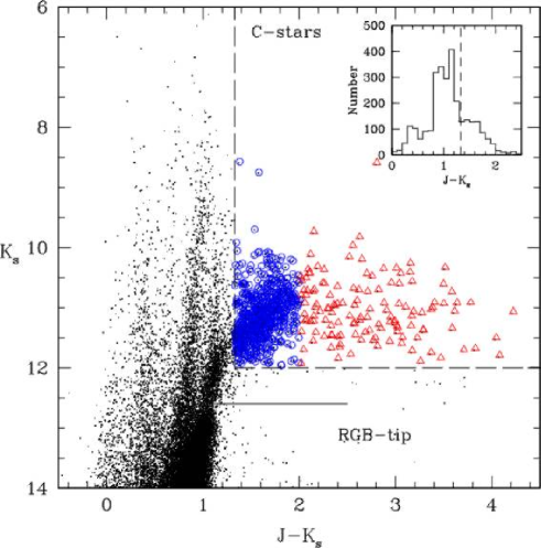
Figure 1: Near–IR CMD of SMC stars from 2MASS within the observed MACHO fields (dots). The C–stars region is marked by two perpendicular dashed lines: C–stars with $J-K_{s}\leq 2$ mag are indicated with blue circles; red triangles refer to obscured AGB stars ($J-K_{s}>2$ mag). The position of the RGB–tip is also indicated. In the upper right corner we show the number of sources with $K_{s}\leq 12$ vs. $J-K_{s}$ colour; note that the branch of C–stars is well separated. See the electronic edition of the Journal for a colour version of the figure.

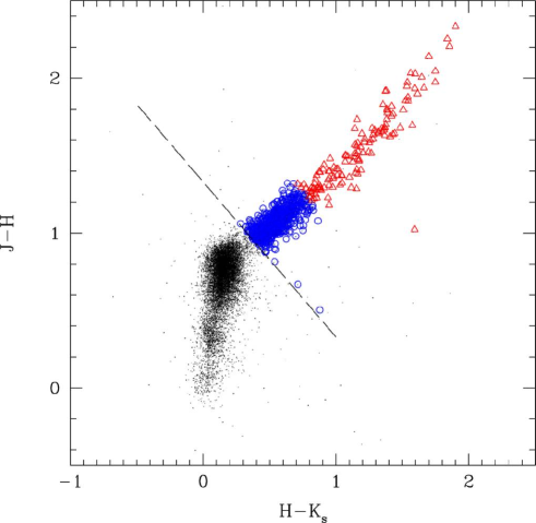
Figure 2: $J-H$ $vs.$ $H-K_{s}$ diagram of SMC stars within the MACHO fields with $K_{s}<14$ mag. The dashed line corresponds to $J-K_{s}=1.33$ mag. Symbols are as in Fig. 1. See the electronic edition of the Journal for a colour version of the figure.

The $\mathrm{MC}^{2}$ catalogue, containing the cross–correlation between DENIS and 2MASS surveys, as well as optical UCAC1 and GSC2.2 catalogues toward the LMC, was published by Delmotte et al. (2002). Here, we use its extension to the SMC (Delmotte 2003) and the near-IR information of the catalogue only. The region confidently populated by C–stars ($J-K_{s}\geq 1.33$ mag and $K_{s}\leq 12$ mag) contains a total of 1657 stars. 805 stars within the MACHO fields satisfy the photometric criterion. The MACHO project observed 6 fields (each of 0.49 deg²), covering the densely populated bar of the SMC of approximately 3 square degrees in total.

Figure 1 shows the near–IR $K_{s}$ $vs.$ $J-K_{s}$ colour–magnitude diagram (CMD) of stars from $\mathrm{MC}^{2}$ and within the MACHO fields. Evolved AGB stars occupy the region above the RGB–tip at $K_{s}\la 12.6$ mag (Cioni et al. 2000) and $J-K_{s}\ \raise-2.0pt\hbox{\hbox to0.0pt{\hbox{$\sim$}\hss}\raise 5.0pt\hbox{$>$}\ }0.97$ mag. At $K_{s}\sim 12$ mag the split into two branches is significant, though it starts already at $K_{s}\sim 12.5$. C–stars populate the well–extended tail toward red colours, while M–stars lie along the almost vertical sequence at $J-K_{s}\sim 1.2$ mag. They reach a maximum luminosity of $K_{s}\simeq 10$ mag, except for 3 stars that have $K_{s}\simeq 9$ and are likely to be more massive O-rich stars (G04). Thus, these 3 have been excluded from the sample. Dust–enshrouded AGB stars are located at redder colours ($J-K_{s}\ \raise-2.0pt\hbox{\hbox to0.0pt{\hbox{$\sim$}\hss}\raise 5.0pt\hbox{$>$}\ }2$ mag). These obscured stars can be either C–rich or O–rich, and spectra are needed to distinguish between the two types. We include them in our analysis, unless they are explicitly rejected by RAW93 (see discussion of contamination by O–rich stars below). The small box in the upper right corner shows the histogram of sources with $K_{s}<12$ $vs.$ $J-K_{s}$ colour. Indeed, the branch of C–stars is well separated from O–rich stars at about $J-K_{s}=1.33$. Other approximately vertical sequences in the main figure at $J-K_{s}\leq 0.97$ are populated by either foreground galactic stars or red supergiants and upper main–sequence stars that belong to the SMC (i.e. Nikolaev & Weinberg 2000).

Figure 2 displays the $J-H$ $vs.$ $H-K_{s}$ colour–colour diagram of the SMC sources within the MACHO fields. This diagram is useful for identifying stars with large infrared excess (Bessell & Brett 1988; Nikolaev & Weinberg 2000). The main feature in the diagram is an extended branch to the right side of the dashed line that marks our selection of C–stars ($J-K_{s}=1.33$ mag). It has been recognized as the locus of TP–AGB stars (e.g. Marigo et al. 2003). Circles and triangles, as in Fig. 1, correspond to stars in our sample. The less populated region at $J-H\ \raise-2.0pt\hbox{\hbox to0.0pt{\hbox{$\sim$}\hss}\raise 5.0pt\hbox{$>$}\ }1.2$ and $H-K_{s}\ \raise-2.0pt\hbox{\hbox to0.0pt{\hbox{$\sim$}\hss}\raise 5.0pt\hbox{$>$}\ }0.8$ mag corresponds to obscured AGB stars. Along this branch a small contamination of stars with $K_{s}>12$ mag is present (small dots). A handful of them might also be C–stars with very large amplitudes caught at minimum light or faint extrinsic C–stars (Westerlund et al. 1995).

2.2 C–stars confirmed spectroscopically

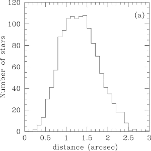
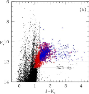
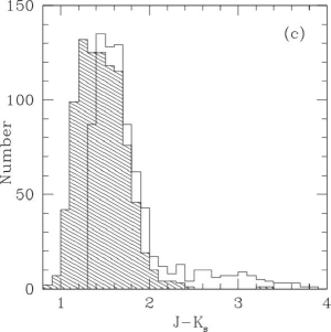
Figure 3: Panel $(a)$: Absolute distance between 2MASS and RAW93 stars in the $\mathrm{MC}^{2}$ catalogue. Panel $(b)$: $K_{s}$ $vs.$ $J-K_{s}$ CMD of all SMC stars in the MACHO field (small black dots). C-stars included in the RAW93 catalogue and within the MACHO fields are plotted as red squares. Blue crosses represent the sample of photometrically selected C-stars. Near–IR photometry comes from the 2MASS survey. Panel $(c)$: histogram of C–stars in our photometrically selected sample (empty) and in the RAW93 catalogue (dashed). See the electronic edition of the Journal for a colour version of the figure.

Our photometric selection criteria of C–stars were checked against the spectroscopically confirmed C–stars in the RAW93 catalogue. Among 1707 stars listed by RAW93 we rejected 27 that were classified by the authors as “doubtful” (flag=1 in Column 8 of their Table 4). Then, we cross–correlated the coordinates of the remaining 1680 C–stars with stars in the entire $\mathrm{MC}^{2}$ catalogue brighter than the RGB tip (i.e. $K_{s}=12.6$ mag), by adopting a searching radius of 3″. The absolute distance between the 2MASS counterpart of the RAW93 sources is shown in Fig. 3$a$. We found that 1275 C–stars in the RAW93 catalogue have a 2MASS counterpart within 3″, and the peak of the distance distribution is at $d\sim 1.2$″. The majority of the spectroscopically confirmed C–stars are well matched to stars in our sample when the same colour and $K_{s}$–magnitude criteria are adopted (see also Cioni et al. 2000). Restricting the area to those fields observed by MACHO, there are 931 C–stars in common between RAW93 and $\mathrm{MC}^{2}$. The location of these stars in the near–IR CMD is presented in Fig. 3$b$.

We find that 73% of 802 C–stars photometrically selected have confirmed C–type spectra. Our photometric selection identifies more C–stars at $J-K_{s}\ \raise-2.0pt\hbox{\hbox to0.0pt{\hbox{$\sim$}\hss}\raise 5.0pt\hbox{$>$}\ }2$ mag with respect to RAW93. This might be because 1) some stars with these colours might be O–rich AGB stars, and 2) some obscured stars were probably below the detection limit in the RAW93 survey. Due to metallicity dependence of the C–star life–time, in a population with the metallicity of the SMC we expect only few of our non-RAW93 stars to belong to the first category. Many spectroscopically confirmed C–stars have a colour bluer than $J-K_{s}=1.33$ mag and a magnitude fainter than $K_{s}=12$ mag, overlapping the region where O-rich stars are also present. These C–stars cannot be disentangled using only a photometric selection criterion (see also G04).

Figure 3$c$ shows the histogram of the number of photometrically selected C–stars versus $J-K_{s}$ colour, together with the number of spectroscopically confirmed C–stars by RAW93 versus $J-K_{s}$. There is a shift between the two distributions suggesting that the spectroscopic identification of C–stars is biased to bluer colours. This is not surprising – in a sample that was spectroscopically selected using CN bands near 8000 Å, Blanco et al. (1980) also found more C–stars with bluer colours than $J-K_{s}=2$.

We find that within the MACHO fields there are 117 stars with $1.33\leq J-K_{s}\leq 2.0$ in the MC² that are not present in the RAW93 catalogue. They amount to 17% of the total number of MC² stars with these colours. Because of the bias discussed above this is an upper limit to the number of O-rich stars contaminating this region of CMD. From comparison with the spectroscopic sample of G04, we also expect the contamination to be low due to the fact that there are only 3 confirmed O-rich stars in the SMC with $(J-K_{s})_{0}=1.30$, $1.58$, and $2.80$, respectively.

Considering the mis–identifications or missed cross–identifications as a result of an automatic association criteria, we estimate a contamination of significantly less than 2.7% and 7.9%, respectively, based on Loup et al. (2003).

2.3 MACHO light–curves

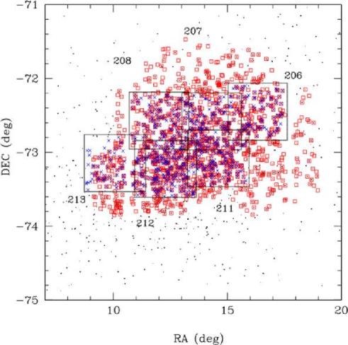
Figure 4: Locations of C–stars in the observed SMC MACHO fields (6 large squares each indicated by its MACHO field number). Small black dots are all photometrically selected C–stars in the SMC; blue crosses refer to C–stars with $|d_{MACHO}-d_{2MASS}|\leq 3$″. Small red squares are C–stars from the RAW93 catalogue cross–correlated with the $\mathrm{MC}^{2}$ catalogue. See the electronic edition of the Journal for a colour version of the figure.

Figure 5: Histogram of the absolute distance between 2MASS sources and their MACHO counterparts. The dashed line is drawn at 3″.

The light–curves of stars in our sample were extracted from the on-line MACHO catalogue. The MACHO project observed the central body of the SMC simultaneously in non–standard (i.e broad) blue ($B_{M}$) and red ($R_{M}$) bands for roughly 8 years (1992–2000). On average there are 800–900 observations per filter for most stars. Since we were interested in the characteristics of the temporal behavior, we used instrumental magnitudes and analyzed the photometric variations in both bandpasses.

Table 1: Cross-identification between the MASTER and MACHO catalogs of our sample of C-stars.

MACHO	DCMC	2MASS	$\alpha$	$\delta$	$d$	RAW93
213.15047.194	J003516.05-732527.7	0035158-732527	8.816091	-73.424309	.100	0
213.15048.4	J003521.86-732422.8	0035216-732422	8.840220	-73.406326	2.400	0
213.15054.264	J003526.42-725835.6	0035263-725835	8.859856	-72.976501	1.150	0
213.15046.550	J003533.80-733032.6	0035337-733032	8.890656	-73.509033	.750	0
213.15051.6	J003537.30-730956.4	0035372-730956	8.905227	-73.165588	.840	0
213.15048.8	J003538.53-732441.3	0035384-732441	8.910099	-73.411438	1.910	0
213.15053.2	J003547.99-730213.7	0035479-730213	8.949644	-73.037003	.430	0
213.15054.103	J003552.13-725834.2	0035520-725834	8.966831	-72.976120	.650	0
213.15105.8	J003603.01-732346.3	0036029-732345	9.012422	-73.396103	1.210	0
213.15106.14	J003612.60-731711.7	0036125-731711	9.052299	-73.286476	.360	0
213.15105.12	J003616.80-732133.1	0036167-732133	9.069947	-73.359169	.660	0
213.15108.5	J003628.84-731144.1	0036287-731144	9.119937	-73.195580	.170	1
213.15108.7	J003630.13-731033.8	0036300-731033	9.125388	-73.175995	.380	0
213.15109.14	J003633.23-730548.0	0036331-730547	9.138298	-73.096611	.320	3
213.15106.12	J003648.03-731830.7	0036479-731830	9.199909	-73.308487	.320	6

2MASS and MACHO coordinates were cross-correlated using a search radius of 3″ and the nearest, and reddest star from MACHO catalogue was chosen as the counterpart to the 2MASS source. Of the 802 photometrically selected C–stars lying within the MACHO fields (Fig. 4), 25 stars were detected twice with different identification numbers because of overlap between adjacent MACHO fields. However, since we chose the nearest star to a 2MASS star as a MACHO counterpart, we avoid double or multiple identifications of the same variable. Nevertheless we did check that the quality of the light–curves is similar. The histogram in Fig. 5 shows the distance in arcsec between a 2MASS source and the corresponding star in the MACHO database. The distribution peaks at $d\sim 0$$\aas@@fstack{\prime\prime}$6, and 65% of the stars are within $d\leq$1″. For 51 stars the nearest MACHO counterpart is at $d>3$″. Of these, 20 are within 10″(6 within 4″) and 31 within 20″. The majority of these stars are located at the edges of the MACHO fields and have poorer astrometry perhaps due to distortions. Moreover, they have bluer instrumental magnitudes than other stars in our sample. Therefore they have been excluded from our analysis. Finally, the photometrically selected sample contains 751 stars with MACHO light–curves.

By cross-correlating the RAW93 and $\mathrm{MC}^{2}$ sample with the MACHO data set, we found that 328 spectroscopically confirmed C–stars are not included in our photometrically selected sample. Thus, the total number of C–star light–curves analysed in the next section is 1079 (751+328).

Table 1 is an extract of the full table, available electronically at Centre de Donn es astronomiques de Strasbourg (CDS), and reports the first 15 lines of the cross-identified MACHO and $\mathrm{MC}^{2}$ sources. It contains: MACHO, DCMC, and 2MASS identifier (Cols. 1-3); right ascension and declination (in degrees) from the second incremental release of the 2MASS catalogue (Cols. 4 and 5); the positional difference between 2MASS and MACHO coordinates in arcsec (Col. 6) and the RAW93 identification number (if appropriate, otherwise 0) (Col. 7).

3 Analysis of Periods and Amplitudes

An independent Fourier analysis of the $B_{M}$ and $R_{M}$ light–curves was performed to search for periodicities in the data. The MACHO time-baseline is about 2700 days, more than twice that of OGLE–II database used, for example, by Ita et al. (2004a, 2004b), Kiss & Bedding (2004) and G04. Resulting periods above 2600 days ($\log P=3.4$) should be considered less significant. Only photometric measurements that are more accurate than 0.1 mag are used. The method that extracts the light–curve parameters is based on the Lomb-Scargle algorithm (Lomb 1976; Scargle 1982) as used by Rejkuba et al. (2003). It is described in Appendix A.1.

Initially 751 light–curves of photometrically selected C-stars were analysed. All the light–curve fits and their parameters were inspected visually. Based on this inspection, and on parameters returned by the light–curve analysis programmes, three quality flags were assigned to each light–curve: $flag(1)$ describes the data quality, $flag(2)$ describes the light–curve fit quality, and $flag(3)$ describes the detected periodicities. Table 2 summarizes flag values and their meaning while more details are given in Appendix A.2 with examples of light-curves associated to a given flag value. Light–curves with $flag(1)\leq 2$ produce reliable period determinations, as confirmed by the fact that for most of them the Fourier analysis has provided good results ($flag(2)\leq 2$). Only for some stars ($8\%$ and $11\%$, respectively, in $B_{M}$ and $R_{M}$ photometry) classified as good light curves ($flag(1)\leq 2$), uncertain periodicity ($flag(2)=3$) or no periodicity ($flag(3)=0$) was detected because of highly irregular light–curves.

Table 2: Description of the values of different $flags$ for the complete sample of 1079 C–stars.

Data Quality			BLUE	RED
$flag(1)$	0	excellent	306	803
	1	good	478	70
	2	fair	136	20
	3	noisy or few data	115	150
	4	no data	44	36
Fit Quality			BLUE	RED
$flag(2)$	0	excellent	124	101
	1	good	191	258
	2	fair	470	349
	3	bad	127	168
	4	underivable	123	167
	5	underivable: $flag(1)$=4	44	36
Detected Periodicity			BLUE	RED
$flag(3)$	0	no periodicity	143	135
	1	1 period	558	608
	2	2 periods	311	292
	3	one period	67	44
		second period uncertain

The same procedure was applied to the 328 stars common to MC², RAW93 and MACHO but missed by the photometric selection. Aliases were identified from the diagram $log\,P$ $vs.$ $K_{s}$ magnitude as those periods that create clear vertical paths (see also Appendix A.1). These correspond to periods equal to 1 and 2 years exactly and were removed from our analysis.

The adopted procedure allowed us to define a semi-automatic algorithm to obtain the light–curve parameters and access their quality. It is summarized as follows: the best fitting period(s) are obtained from Eq. A.1; the quality of the observations is derived from $flag(1)$; the quality of the period determination is evaluated using the spectral power that is closely related with a semi-automatic definition of $flag(2)$ (Appendix A.2). Note that this procedure can also be applied to stars of a different type (i.e. M–type stars) in the MACHO catalogue or to other measurements of stellar variability in a comparable sampling.

Amplitudes related to the main periodicity of light–curve variations were determined both from the sinusoidal fit of each light-curve and from the peak-to-peak magnitude difference. A comparison of both determinations is given in Appenxix A.3.

Figure 6: Comparison between the period and amplitude derived in this work and those from Cioni et al. (2003).

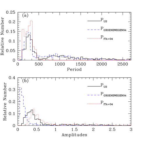
Figure 7: Comparison between the period and amplitude derived in this work and those from Ita et al. (2004b) and G04.

3.1 Results and statistics

Table 3: Light curves parameters: $X$ is the mean magnitudes; first (second) row refers to $B_{M}$($R_{M}$)-light curve.

MACHO	$<X>$	$A_{1}$	$B_{1}$	$A_{2}$	$B_{2}$	$P_{1}$	$P_{2}$	${\cal P}_{1}$	${\cal P}_{2}$	$A_{phot}$	$flag(1)$	$flag(2)$	$flag(3)$
213.15047.194	.000	.000	.000	.000	.000	.000	.000	.000	.000	.00	3	4	0
	.000	.000	.000	.000	.000	.000	.000	.000	.000	.00	2	4	0
213.15048.4	-8.139	.020	-.077	.027	-.020	1002.284	199.586	102.100	46.200	.26	0	1	2
	-9.629	.060	.011	.000	.000	1658.224	.000	83.200	.000	.16	0	2	1
213.15054.264	.000	.000	.000	.000	.000	.000	.000	.000	.000	.00	4	5	0
	-5.808	-.743	-.917	-.300	.776	1696.516	359.045	178.700	96.400	1.91	1	0	2
213.15046.550	.000	.000	.000	.000	.000	.000	.000	.000	.000	.00	4	5	0
	.000	.000	.000	.000	.000	.000	.000	.000	.000	.00	3	4	0
213.15051.6	-7.740	1.051	.479	.000	.000	621.195	.000	319.800	.000	2.48	1	1	1
	-9.615	.589	.598	.000	.000	611.472	.000	235.600	.000	1.59	0	1	1
213.15048.8	-7.242	.154	.025	.000	.000	171.377	.000	157.200	.000	.50	1	1	1
	-8.822	.104	.062	.000	.000	171.699	.000	114.900	.000	.30	0	1	1
213.15053.2	-6.844	.195	.133	.069	-.111	857.187	230.560	221.400	65.800	.57	1	1	3
	-8.804	.153	.093	.061	-.057	870.538	230.751	248.100	69.100	.44	0	1	2
213.15054.103	.000	.000	.000	.000	.000	.000	.000	.000	.000	.00	4	5	0
	-6.303	.261	1.009	.103	-.953	406.026	2287.050	123.900	97.300	1.73	2	0	2
213.15105.8	-7.505	-.417	-.014	.000	.000	876.287	.000	307.400	.000	1.11	1	1	1
	-9.279	-.339	-.027	.000	.000	873.740	.000	220.800	.000	.61	0	0	1
213.15106.14	-7.132	-.232	.085	.147	.010	294.109	151.497	163.500	51.300	.59	1	1	3
	-9.088	.005	-.138	-.108	.017	260.586	300.278	80.000	69.800	.32	0	2	3

Table 3 lists the parameters derived from our analysis for a total of 1079 stars. Only the first ten lines are shown in this paper, but the complete table is accessible electronically via CDS. The table contains: MACHO identifier (Col. 1); the quantities of the period–amplitude analysis for $B_{M}$ (first row) and $R_{M}$ (second row) light curves: (Cols. 2-9): mean magnitude $X_{0}$, $A_{1}$, $B_{1}$, $A_{2}$, $B_{2}$, $P_{1}$, and $P_{2}$ in days, power strength of the first ${\cal P}_{1}$ and second period ${\cal P}_{2}$; $A_{phot}$ (Col. 10) $flag(1)$, $flag(2)$, and $flag(3)$ values (Col. 11-13). Among the 1079 stars the following have passed the data–quality criterium $flag(1)\leq 2$: 919 $B_{M}$ and 893 $R_{M}$ light-curves.

In the following discussion, only the good 919 $B_{M}$ light-curves are used, unless explicitly stated otherwise. Within this sample 785 stars also have $flag(2)\leq 2$ and a minimum amplitude of 0.05 mag, thus are all variables. About 4% show a very regular variation with only one periodicity. The others appear multiperiodic. Some (7%) show a well–defined first period with amplitude variations and a less clear second periodicity, while others (59%) clearly show two periods (examples are given in Fig. 18).

The availability of accurate photometry and long–term observations has made the distinction between regular and semi–regular (SR) variables more and more difficult (Whitelock et al. 1997). The stellar light–curves can be as regular in SR as in Mira class, but on average SR variables show smaller amplitudes (Cioni et al. 2003). However, due to a difficult and rather subjective classification we only distinguish between two broad groups: sources which show a clear single periodicity and sources which are multiperiodic. About 15% appear to be irregulars ($flag(2)=3$), with no clear period.

Table 3 has 131 stars are in common with Cioni et al. (2003). Fig. 6$a$ shows the comparison between the periods derived in the present paper and those in Cioni et al. (2003). Amplitudes are compared in Fig. 6$b$. We plotted stars with $flag(2)\leq 2$ in our analysis and stars with $Flag<9$ and $Flag\neq 5$ in the table by Cioni et al. (2003). There are 78 stars in common. The mean period and amplitude differences are: $P_{present}-P_{Cioni03}=-14\pm 76$ and $A_{present}-A_{Cioni03}=-0.9\pm 0.8$. The periods agree within the uncertainty in the period determination that is on the order of 5%, except for few stars for which Cioni et al. (2003) derive only one period and flag the LPV as multiperiodic, while we find 2 periods that are typically shorter. It is possible that additional longer periods are present as well. In contrast, amplitudes are systematically different. Note that Cioni et al. (2003) define amplitude as the difference between the minimum and maximum value of MACHO photometry, which is different from our definition of $A_{phot}$ (see Appendix A.3). This could explain why Cioni et al. amplitudes are systematically larger than ours.

Figure 7 shows the comparison between periods and amplitudes as derived in the present paper and those by Ita et al. (2004b) and G04. In both panels, for all the three works only stars satisfying our photometric criteria are reported. In Fig. 7$a$ in the case of multi–periodic variables the period of G04 corresponding to the largest amplitude and our first period are reported. Ita et al. (2004b) only give the predominant period and do not analyze multi–periodic light–curves. The present results are in good agreement with those by G04, predicting periods as long as 2400 d, while Ita et al. (2004b) do not find periods longer than about 690 d.

In Fig. 7$b$ the OGLE $I$–band amplitudes of Ita et al. (2004b) and G04 are compared with the present $R_{M}$–band amplitudes as derived from the light–curves ($A_{phot}(R_{M})$, see Appendix A.1). In the case of G04 we plot the largest amplitudes from his Table 2. Although a direct comparison between $R_{M}$– and $I$–band amplitudes is difficult, the shape of the histogram illustrating our results is similar to that by Ita et al. (2004b), even if we have a larger number of stars with amplitudes smaller than $\sim$0.4. G04 found that the majority of C–stars in his sample have $\Delta I<0.2$, while Ita et al. (2004b) have almost no stars in the same amplitude range.

Both Fig. 6$b$ and Fig. 7$b$ indicate that the various methods for estimating pulsation amplitudes can give systematically different results (see also Appedix A.3). Ita et al. (2004b) and Cioni et al. (2003) derive pulsation amplitudes as $\Delta X=X_{max}-X_{min}$, where $X$ is the photometric band used, while G04 estimate amplitudes from the sinusoidal fit.

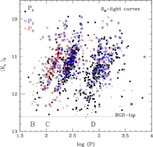
Figure 8: $\langle K_{s}\rangle_{0}$ $vs.$ $logP$ relation for all C–stars in the sample (small black dots). Large dots are first periods ($P_{1}$) for stars with $flag(2)\leq 2$ and $flag(3)=1$; blue open squares $P_{1}$ for stars with $flag(2)\leq 2$ and $flag(3)=2$ and 3; red crosses correspond to the second period ($P_{2}$) of stars indicated by squares. The $\langle K_{s}\rangle_{0}$ magnitude is the average of DENIS and 2MASS measurements, dereddened as explained in the text. Letters identify the parallel sequences as defined by Wood et al (1999).

Figure 9: Histogram of all the periods found for $B_{M}$ light–curves, though for $R_{M}$ light–curves results are very similar. The empty histogram shows the distribution of P₁ and the shaded histogram of P₂. Letters indicate sequences as in Wood et al. (1999).

4 Discussion

4.1 Log(P) vs. $K$ diagram

In the past five years new results for the log(P) vs. $K$–band mag diagram have been obtained as a by–product of microlensing projects such as MACHO, OGLE, and EROS. Wood et al. (1999) found that the bright red giant variables in the LMC form four sequences: three are the result of different pulsation modes and one, at the longest periods (seq. D or the long secondary period sequence – LSP), remains unexplained. Ita et al. (2004b) showed that some sequences possibly split into sub–sequences at the discontinuity around the tip of the RGB. G04 analyzed spectroscopically confirmed M– and C–type stars and concluded that the LSP sequence is independent of evolutionary and chemical (C–rich or O–rich) effects. A comparison of the SMC and the LMC sequences can also be found in Cioni (2003). More recently, Schultheis, Glass, and Cioni (2004) compared variable stars in the different sequences between the Magellanic Clouds and the NGC6522 field in the Galaxy. These authors conclude that all three fields contain similar types of variables, but the proportion of stars that vary decreases at lower metallicities and the minimum period associated with a given amplitude gets longer.

Figure 8 shows the distribution of the mean $\langle K_{s}\rangle_{0}$ mag vs. the logarithm of the period obtained by analyzing $B_{M}$ light–curves. However, the discussion that follows applies also to a similar analysis of $R_{M}$ light–curves. In fact as expected from the comparison shown in Fig. 21, there are no differences in the periods obtained from the two channels.

In Fig. 8 all sources in the sample are indicated by small black dots. In addition, stars for which only one reliable period was detected ($flag(2)\leq 2$ and $flag(3)=1$) are plotted as larger dots, while for stars with two reliable periodicities detected ($flag(2)\leq 2$ and $flag(3)=2$ and 3), the first and the second periods are plotted with blue open squares and red crosses, respectively. The $K_{s}$–band photometry is the mean of DCMC and 2MASS measurements ($\langle K_{s}\rangle$). DCMC magnitudes are corrected for the shift in the absolute calibration according to Delmotte et al. (2002). The $K_{s}$–magnitude is also dereddened according to a SMC mean reddening of $E(B-V)=0.065\pm 0.05$ obtained by averaging different measurements (Westerlund 1997). By adopting the extinction law of Glass (1999) and $R_{V}=3.1$ we obtain $A_{K_{s}}=0.02$ and $A_{J}=0.05$.

All periods range in the interval 1.5  $\sim$$<$  log(P)  $\sim$$<$  3.5 (Fig. 8). There are 3 well-defined parallel sequences in the PL diagram with a small number of stars lying between the sequences. Part of the scatter is due to the fact that the $K_{s}$–band is a mean of only 2 measurements and part is due, probably, to depth effects in the SMC. The line of sight depth of the SMC is estimated to range between 5–20 kpc by various authors (Westerlund 1997). Hence, assuming the SMC distance modulus of (m-M)=19 mag and the full depth of 10 kpc, we expect a scatter on the order of $\sim 0.4$ mag around the average.

Sequences can be identified with B, C, and D from Wood et al. (1999). It is interesting to note that C-stars do not populate shorter sequences (i.e. sequence A), a result already visible from Fig. 4 of Ita et al. (2004b), and noted in the LMC by Fraser et al. (2005). Since the baseline explored here is longer than that of previous works (except for Fraser et al. 2005 who analysed MACHO data in the LMC), we find a well populated D sequence, about 34% of the variable stars in our sample have a first or second period longer than 630 days. This should be compared with previous results which found ($i$) 25% of all variable AGB stars in the LMC (Wood et al. 1999), but with a very small fraction belonging to C-rich LPVs (Fraser et al. 2005), and ($ii$) 24.6% of all the spectroscopically selected C-stars with periods from OGLE-II photometry in the SMC on the sequence D (G04). The bias against detection of variables with periods in excess of $\sim 800$ days in the latter work may be why we find more C-stars on this sequence. This shows that very long–term monitoring is essential. Even in the case of our sample from MACHO with an 8-year time–baseline, it is not clear if the drop in the period distribution at $\log\,P\sim 3.3$ is real or an artifact due to incompleteness at longest periods (see Fig. 9).

Sequence D is much broader than the others, and the nature of its stars is still a matter of debate Wood et al. (2004). Only a few of them, those with $J-K_{s}>2$ (see Sect. 4.5) are probably dust-enshrouded AGB stars that could have either carbon or oxygen-dominated chemistry, but their number is very small. Thus, as already concluded by Wood et al. (2004) from the similarity of the colour variations associated with both the primary and secondary periods, dust is unlikely to cause the LSPs. Clearly, a long-term spectroscopic and photometric monitoring of these stars is necessary to gain some insight into the nature of their variability.

In Fig. 9 we compare the histogram of the first detected periods, which represent the dominant periodicity in a given star, with the second best period. First periods mainly occupy sequences $C$ and $D$ with the peaks at $log\,P=2.45$ and $log\,P=2.95$, respectively. Second periods mainly populate sequence $B$ and peak at $log\,P=2-2.3$. A weak peak is also seen at $log\,P=3.2$, which is clearly part of sequence $D$.

4.2 Log(P) vs. period ratio

According to Lattanzio & Wood (2003) a star that evolves up the AGB first pulsates at low amplitude on sequence A, then with further evolution the sequence B mode will become unstable and its amplitude increases, while the sequence A mode amplitude decreases. The star will be a multi–mode pulsator having periods in sequences $A$ and $B$. The pulsation amplitude of each mode increases with increasing stellar radius. Subsequently a fundamental mode in sequence $C$ will also become unstable. At this moment up to three different periods of pulsation can be detected in a given star. However, the competing growth rate of the amplitude of each pulsating mode may shade the detectability of a given periodicity. For example for a $1M_{\odot}$ star the fundamental period dominates at $M_{bol}>-4.5$, while at $M_{bol}<-3.5$ the first and second overtone pulsation modes are stronger. The star will finally end up as a dust–enshrouded, large amplitude fundamental mode pulsator prior to ejection of all its envelope and the beginning of the Planetary Nebulae phase.

For stars with detected multiperiodicity we plot the ratio between the longer to the shorter period as a function of the longer one in Fig. 10. A well–defined group of stars have ratios ranging from 1 to 2. These are shown in zoom–in in the upper left corner of the figure. They belong to the sequence $C$ (longer) and $B$ (shorter) periods. Their ratio distribution agrees with the scenario proposed by Lattanzio & Wood (2003) for a star pulsating in the fundamental, first and second overtone (see their Fig. 53). An extended tail up to a ratio of 20 is populated by stars with the longer period on sequence $D$ and the shorter period along either sequence $C$ or $B$. There are no theoretical models available at present to explain these high ratios which involve an intrinsic stellar pulsation; thus a different nature for long–term modulation needs to be invoked. It is interesting to note that most of the sources with $P_{1}<P_{2}$ have lower period ratios and slightly larger values of longer periods with respect to sources with $P_{1}>P_{2}$.

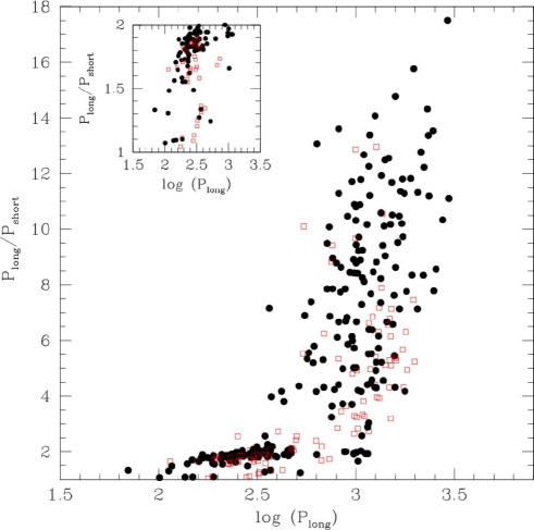
Figure 10: The ratio between the longer to the shorter period versus the longer period. Black–filled circles represent stars with $P_{1}>P_{2}$, while red open squares sources with $P_{1}<P_{2}$. In the upper left corner we show an enlargement of the lowest ratios.

4.3 Log(P) vs. amplitude

Figure 11 shows the period distribution (of only the first periods $P_{1}$) as a function of amplitude in the MACHO bands. Most variables have amplitudes in the optical bands below about $0.5$ mag. Stars that occupy sequences $C$ and $D$ are clearly separated. Sequence $B$ is not present in these diagrams because it is mostly populated by secondary periods. It should be also noted that amplitudes belonging to secondary periods are typically smaller, and thus this figure should be compared with those of other authors (e.g. G04, Ita et al. 2004b) with caution. In addition, the definition of amplitude is not always a trivial issue with these highly variable stars that often have variable amplitudes as well. We discuss this in Appendix A.3. Here we use amplitudes determined directly from photometry ($A_{phot}$) as defined in Appendix A.3.

Both $C$ and $D$ sequences present distribution tails to large amplitude (from a few tenth up to 3 mag) values that probably correspond to variables of Mira type. While Miras typically occupy sequence $C$, a few of them can be found on sequence $D$ because they have fainter magnitudes due to dust obscuration.

Figure 12 shows the period distribution for small ($0.05\leq A_{phot}(B_{M})\leq 0.2$; open histogram) and large ($A_{phot}(B_{M})>0.2$; shaded histogram) amplitude variables. The two distributions are different. Small amplitude variables have two peaks that correspond to the period–magnitude relations $C$ and $D$. Large amplitude variables are more homogeneously distributed between $log(P_{1})=1.6$ and $3.1$. Fewer of them have longer periods, though at $\log\,P\ga 3.1$ the sample might be incomplete.

In Schultheis, Glass & Cioni (2004) the period of both small and large amplitude variables defined as in Fig. 12 increases progressively with decreasing metallicity, even though the general period distribution of the two classes is fairly similar. In the present paper stars located in sequence $C$ ($1.9\leq log(P_{1})\leq 2.7$) span the full range of periods if they are either small or large amplitude variables. Therefore there seems to be no indication of a difference in metallicity between the small and large amplitude LPVs on this sequence. On the other hand, the majority of large amplitude variables that occupy sequence $D$ ($2.7\leq log(P_{1})\leq 3.5$) have $log(P_{1})\leq 3.1$. A longer monitoring time–baseline is necessary to discern whether this lack of longer period large amplitude LPVs on sequence $D$ is real or due to incompleteness, and thus if it could represent shortage of lower metallicity stars among the large amplitude variables.

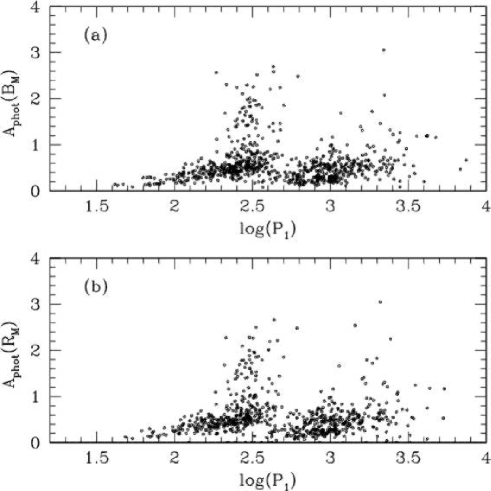
Figure 11: Period distribution as a function of amplitude in the two MACHO photometric bands.

Figure 12: Period distribution ($log(P_{1})$) of stars with $0.05\leq A_{phot}(B_{M})\leq 0.2$ (empty) and $A_{phot}(B_{M})>0.2$ (shaded).

4.4 Log(P) vs. $J-K_{s}$ colour

Figure 13 shows that redder variables have a larger amplitude. In fact Ita et al. (2004b) also found that the C–rich regular pulsators (Miras) have larger amplitude the redder the star, while the O–rich Miras seem to have arbitrary amplitudes as a function of $J-K_{s}$ colour. When the $J-K_{s}$ colour gets redder, periods increase for variables in the $C$ sequence (see Figure 13$b$). This is apparently not the case for stars populating the $D$ sequence, which again indicates a different mechanism is responsible for the light–curve variations.

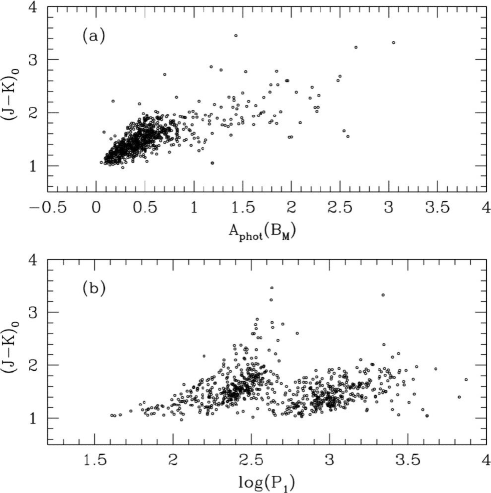
Figure 13: $(J-K_{s})_{0}$ vs. the $B_{M}$-band amplitude $(a)$ and vs. $log\,(P_{1})$ $(b)$ for all C–stars.

4.5 Properties of stars on the $BCD$ sequences

We found no difference in the location of stars belonging to the $BCD$ sequences in the $K_{s}$ vs. $J-K_{s}$ diagram. In Fig. 14 we investigated the $K_{s}$ luminosity function and $J-K_{s}$ colour distribution of stars in each sequence for both the first (empty histogram) and second (shaded histogram) detected periods. Most of the stars with $J-K_{s}>2$ belong to sequence $C$, and they have only one detected and dominant periodicity. A handful of them show a long second period in sequence $D$. The faintest stars analyzed in this sample ($12\leq K_{s}\leq 12.6$) have their first period either in sequence $B$ or $D$ and eventually a second period in sequence $C$, which is often the case for stars in sequence $D$ that are multi–periodic, while stars in sequence $B$ usually have only one period detected. The bulk of the C–star population has a first period that occupies sequence $C$ or $D$ and somewhat less sequence $B$, which is instead largely populated by the second period of these same stars.

Figure 14: Distribution of the number of sources populating each $BCD$ sequence versus $K_{s}$ magnitude and versus $J-K_{s}$ colour. The empty histogram indicates the first period ($P_{1}$) and the shaded histogram the second period ($P_{2}$).

4.6 Log(P) vs. $M_{bol}$

Figure 15 shows the PL–relation for all stars in the sample. Overplotted are the theoretical models by Vassiliadis & Wood (1993) for different masses and a mean SMC metallicity of $Z=0.004$. To transform $K_{s}$ magnitudes into $M_{bol}$ we used the relations by Bergeat, Knapik, & Rutily (2002). Their Fig. 1 shows that the bolometric correction is well–defined for C-stars with $J-K_{s}\ \raise-2.0pt\hbox{\hbox to0.0pt{\hbox{$\sim$}\hss}\raise 5.0pt\hbox{$<$}\ }2.1$, while for increasing colours the uncertainty becomes larger. In our sample of 1079 stars, only 30 have $(J-K_{s})_{0}>2.1$ and $flag(2)\leq 2$, these sources are emphasized in Fig. 15 as green triangles. These stars have large amplitudes (see Fig. 13) which is likely to influence their location in Fig. 15.

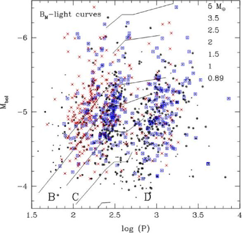
Figure 15: $M_{bol}$ $vs.$ $logP$ relation for all stars in the sample and overplotted theoretical tracks by Vassiliadis & Wood (1993). Green triangles indicate stars with $(J-K_{s})_{0}>2.1$ and $flag(2)\leq 2$, while other symbols are as in Fig. 8. Masses are indicated on the right hand side of each track. See the electronic edition of the Journal for a colour version of the figure.

A comparison of the PL diagram with the models in Vassiliadis & Wood indicates that the bulk of C-rich LPVs in the SMC have lower masses than 2.5-3 M_⊙, which at the metallicity of the SMC corresponds to ages of 0.5-0.3 Gyr (Pietrinferni et al. 2004). This agrees with the SFH derived by Harris & Zaritsky (2004), who found an active star formation during the past 3 Gyr with three enhanced episodes at 2.5, 0.4, and 0.06 Gyr. Few carbon stars show higher masses up to 5 M_⊙ corresponding to an age of $\sim$0.1 Gyr.

4.7 Spatial distribution

The spatial distribution of stars in each sequence is investigated. There seems to be no indication of a spatial correlation between stars that occupy one or the other sequence in the period–magnitude diagram with their location in the galaxy. We also checked if there is any difference in the spatial distribution of stars where different masses were expected. Again, we do not find clear indication of a different distribution of sources with a different initial mass. There are overall less sources with high mass (or young), and a lack of these sources in the Northeast, Northwest and Southwest regions compared to other locations in the galaxy. The distribution of sources with intermediate and low mass is fairly similar.

5 Summary and conclusions

This work analyzes and discusses the MACHO light-curves of 1079 C–stars. The sample consists of 751 photometrically selected stars from the MC² catalogue according to $J-K_{s}\geq 1.33$ mag and $K\leq 12$ mag criteria, and 328 spectroscopically confirmed C-stars from RAW93 catalogue. Many of the photometrically selected sample also have C-type spectra (RAW93), meaning that for 18% of all the sample we do not know their spectral type. However, given the low metallicty of the SMC and a very low number of spectroscopically known O-rich AGB stars in the SMC (G04), we expect the contamination by O-rich AGB stars to be negligible. For all the stars, we performed Fourier analysis of their light–curves identifying up to 2 significant periodicities.

All the stars for which good quality light-curves exist were found to vary with amplitudes of at least 0.05 mag in the two MACHO photometric bands. The analysis was carried independently for $B_{M}$ and $R_{M}$ light–curves, and the derived periods are identical (to within the errors). After a selection based on the quality of the light–curve, significance of the derived periods, and quality of the periodicity fits, a total of 919 C–stars were used in further analysis.

Carbon stars occupy bright parts of sequences $B$, $C$, and $D$ in the $K_{s}-\log\,P$ diagram. None of the stars in our sample have shorter periods characteristic of sequence $A$, which is in agreement with recent studies by Fraser et al. (2005) in the LMC, and Ita et al. (2004a,b), and G04 who observed this in the SMC as well. The large majority of the stars have their primary (dominant) periodicity on sequence $C$ or $D$, while more than 2/3 of sequence $B$ is populated by secondary periods of those stars whose primary period is on sequences $C$ or $D$. The stars whose primary period is on sequence $B$ are preferentially fainter and bluer. This is in agreement with the models that predict change of pulsation mode for the LPVs from higher overtones towards a fundamental mode as they evolve along the AGB (e.g.  Lattanzio & Wood 2003).

Most of the stars with $J-K_{s}>2$ belong to sequence $C$, and only a handful of these reddest variables show a long second period in sequence $D$. This is a clue that dust obscuration cannot be a cause of the long secondary periods (see Wood et al. 2004, for a detailed discussion). The luminosity functions of the three sequences span a similar range of magnitudes, but the faint distribution tail of sequence $D$ is more populated. Again, we cannot explain it with the dust obscuration, as there are very few stars redder than $J-K_{s}>2$ on this sequence. The width of this sequence in the period–magnitude diagram is larger than that of other sequences, especially at brighter magnitudes, but the lack of stars with a period longer than ($log\ P\sim 3.5$) may be due to incomplete time coverage.

Stars belonging to different pulsational sequences are homogenously mixed over the SMC area. Their masses were derived from a comparison with the theoretical tracks of Vassiliadis & Wood (1993), and the majority of them are indicative of the major star formation episode that took place $\sim 0.3-0.5$ Gyr ago. This is in excellent agreement with Harris & Zaritsky (2004), who found enhanced star formation episodes at 2.5, 0.4, and 0.06 Gyr in the SMC. However, our sample indicates a considerably weaker star formation event at younger ages ($\sim 0.1$ Gyr ago), which is expected as these younger, and thus more massive, stars are preferentially oxygen-rich, hence not in our sample. There is no clear difference in the spatial distribution of the stars with different masses.

The very long–time baseline of MACHO observations has allowed us to confidently extract long periods up to ($log\ P\sim 3.5$). We found that about 10% of the variables fall on sequence $B$, 30% on $C$, and 34% on $D$. The latter percentage is higher than the 25% derived by Wood et al. (1999) and than the 21% derived by G04 in the LMC. It is also important to note that in the LMC, Fraser et al. (2005) find only a small fraction of probable C-stars with periods along sequence $D$. Monitoring of these variables over more than an 8–year period photometrically and spectroscopically is desirable in order to discern their nature. According to Wood et al. (2004) these stars belong to the only class of bright large amplitude variables whose properties cannot be explained with theoretical models at present.

Appendix A Determination of Periods and Amplitudes

A.1 Method

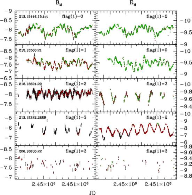
Figure 16: Examples of light–curves with different values of the data–quality $flag(1)$. Data with photometric errors $0.05\leq\sigma_{X}<0.1$ are plotted as black dots; data with $0.01\leq\sigma_{X}<0.05$ are plotted as red squares; and data with $\sigma_{X}<0.01$ as green crosses. Left (right) panels illustrate $B_{M}$ ($R_{M}$) photometry. See the electronic edition of the Journal for a colour version of the figure.

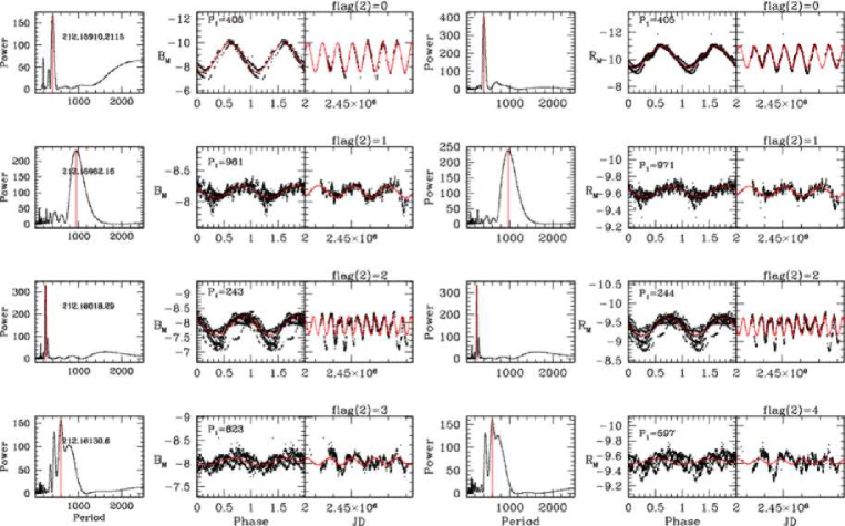
Figure 17: Examples of light–curves with different values of $flag(2)$. Left (right) panels illustrate $B_{M}$ ($R_{M}$) photometry. For each band we show the periodogram and the light–curve in the phase and time domain. See the electronic edition of the Journal for a colour version of the figure.

The method used to determined the first period is already discussed in Rejkuba et al. (2003). To detect the second period we used the following fitting function:

$$X(t) = A_{1}\cos\left(2\pi\frac{(t-t_{0})}{P_{1}}\right)+B_{1}\sin\left(2\pi\frac{(t-t_{0})}{P_{1}}\right)$$

$$+ A_{2}\cos\left(2\pi\frac{(t-t_{0})}{P_{2}}\right)+B_{2}\sin\left(2\pi\frac{(t-t_{0})}{P_{2}}\right)$$

$$+ X_{0}$$

where the first guess for the second period comes from the second, or sometimes the third, strongest peak in the power spectrum. Usually, the first period is obvious, while secondary peaks are less clear. We noted that semiregular and irregular light curves show several peaks in their Fourier spectrum with similar strength. Usually we followed the strength sequences of the power values to define the second period. However, the amplitudes of the peak are just a starting point. In fact we always inspected the relative results by eye, in order to check the reliability of the second assigned period. In some cases we considered the third peak more appropriate than the second, which could be instead an alias (a false period which seemingly fits the data, as well as the correct period). The alias frequencies $\nu_{a}$ are related to the true frequency $\nu_{t}$ by $\nu_{a}=\nu_{t}\pm n/(\Delta t)$, where $\Delta t$ is the spacing in days between the measurements. The pattern of the aliases will therefore depend on the true period and the particular $\Delta t$ for the star in question.

We call the first period ($P_{1}$) the best fitting period obtained from the first term of Eq. A.1 and ${\cal P}_{1}$ the associated value of the power. We call the second period ($P_{2}$) the best fitting period obtained from Eq. A.1 and ${\cal P}_{2}$ the associated value of the power. Amplitudes ($A_{fit}$) associated with the first period are defined from the sinusoidal fit as:

$$A_{fit}=2\times\sqrt{A_{1}^{2}+B_{1}^{2}},$$ (2)

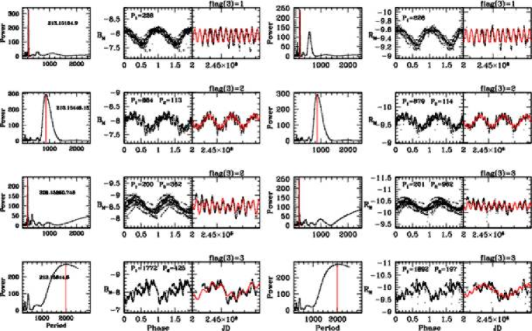
Figure 18: As in Fig. 17, but for $flag(3)$.

A.2 Quality assessment

Table 2 summarizes the values of the three quality flags associated to each light-curve and the number of light-curves with a given value. In particular, $flag(1)$ is related to the accuracy of the photometric measurements. We defined $n_{0.05}$ and $n_{0.01}$ as the ratio between the number of observations with, respectively, magnitude error $\sigma_{X}<0.05$ and $<0.01$ and the total number of measurements in each light–curve (i.e.  with magnitude errors $\Delta<0.1$). Thus, values to $flag(1)$ are assigned as follows:

$$flag(1) = 0\>\>\>if\>\>\>n_{0.01}\geq 0.7\>\>\>\>\>\>(excellent)$$

$$flag(1) = 1\>\>\>if\>\>\>0.5\leq n_{0.05}<1\>\>\>and\>\>\>0.1\leq n_{0.01}<0.7\>\>\>$$

$$\>\>\>(good);$$

$$flag(1) = 2\>\>\>if\>\>\>0.5\leq n_{0.05}<1\>\>\>and\>\>\>n_{0.01}<0.1\>\>\>$$

$$\>\>\>(fair);$$

$$flag(1) = 3\>\>\>if\>\>\>n_{0.05}<0.5\>\>\>and\>\>\>n_{0.01}<0.05\>\>\>$$

$$\>\>\>(few\>or\>noisy\>data)$$

A sample of light–curves of different types, together with the associated $flag(1)$, is shown in Fig. 16. The algorithm works well; only for a handful of cases the inspection by eye has revealed that data are sparse over several magnitudes even if they have very small magnitude error. In these cases we re–assigned $flag(1)=3$. The majority of light–curves classified as $flag(1)=2$ look like 213.15624.20 $B_{M}$-light curve in Fig. 16. Only in a few cases are very regular and large amplitude LPVs classified with $flag(1)=2$ or even 3 (see for example 213.15332.2889, $B_{M}$, and $R_{M}$ light–curve in the Fig. 16).

The fit quality flag ($flag(2)$) and the periodicity flag ($flag(3)$; see Table 2) are less objective and much more related to an inspection by eye than $flag(1)$. In order to assign values to these flags, first we carefully eye–inspected the first period in the phase and time diagrams. Then, we looked at the combined periodicities (Eq. A.1). On the basis of these inspections we assigned values for $flag(2)$ and $flag(3)$ according to Table 2. In Fig. 17 we plot light–curves with different values of $flag(2)$ referring only to their first periodicity. Fig. 18 illustrates examples of light–curves with different values of $flag(3)$. In both figures for each star we plot the corresponding power spectrum and the light curve in phase and time domain and overplot the best fitting sinusoidal function.

Figure 19: Histogram of the power of the first period ($B_{M}$–light curves) as a function of the defined fit-quality flag. The relative number of stars is indicated in each panel.

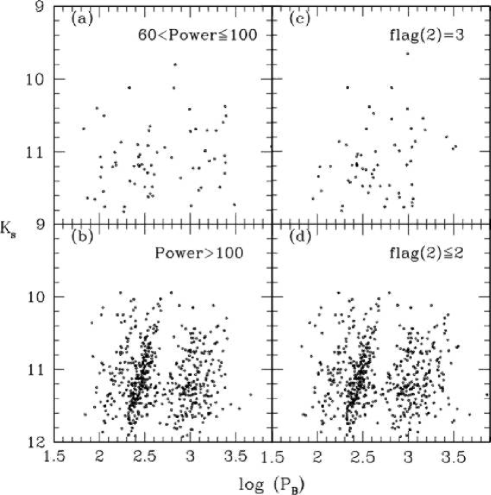
Figure 20: Distributions of the first period ($B_{M}$–light–curves) as a function of the power value (left panels) and $flag(2)$ (right panels).

In order to provide an automatic classification of the fit quality, we analyzed the correlation between $flag(2)$ and the strength of the power of the first period (${\cal P}_{1}$) as follows. In Fig. 19 the histogram of ${\cal P}_{1}$ is reported for different values of $flag(2)$. It is clear that starting from $flag(2)=0$ to $flag(2)=4$ the peak of the distribution moves toward lower power values. In particular, for $flag(2)=0$ and 1 (Fig. 19$a$) the only region populated is that with ${\cal P}_{1}\geq 100$; the bulk of variables with $flag(2)=2$ have ${\cal P}_{1}\ \raise-2.0pt\hbox{\hbox to0.0pt{\hbox{$\sim$}\hss}\raise 5.0pt\hbox{$>$}\ }100$ with only a small number of stars with ${\cal P}_{1}<100$. The distribution of variables with $flag(2)=3$ peaks in the range $80\leq{\cal P}_{1}<100$, and those for which no satisfactory period could be derived mainly have ${\cal P}_{1}<40$.

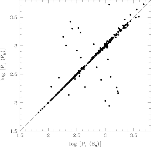
Figure 21: Relation between the first periods derived from $B_{M}$ and $R_{M}$ light–curves.

Figure 20 emphasizes the good correlation between these two quantities. In panels ($a,b$) we plot $log(P)$ vs. $K_{s}$ (see next section for a discussion) for stars with $60<{\cal P}_{1}<100$ ($a$) and stars with ${\cal P}_{1}>100$ ($b$). Panels ($c,d$) show the same quantities but for stars with $2flag(2)=3$ $(c)$, and $flag(2)\leq 2$ ($d$). We conclude that the selection described in panels ($b,d$) outlines three sequences and the distribution of stars in both panels are very similar. These results are related to $B_{M}$ light–curves, however an inspection of $R_{M}$ light–curves gives similar results. Fig. 21 shows an almost perfect correlation between the first period obtained from $B_{M}$ and $R_{M}$ light–curves. Only stars with $flag(2)\leq 2$ are plotted. For 94% of the objects the residual dispersion of the differences is lower than 4%. Only a few points scatter away from the 1:1 line, implying that the primary period is the same in both bands. Most of these points occur because the first period (here ${\cal P}_{1}$) found from the $B_{M}$ light–curve corresponds to the second period (${\cal P}_{2}$) found from the $R_{M}$ light–curve, and confronting only ${\cal P}_{1}$ between both light–curves produces a point that does not follow the correlation. A few other points occur when the period ${\cal P}_{1}$ derived from the $B_{M}$ light–curve is twice that derived from the $R_{M}$ light–curve.

Summarizing, an automatic selection criterion (i.e. by using ${\cal P}_{1}$) can be applied with a good level of confidence for the analysis of the primary periods of a large sample of variables.

To define $flag(3)$ in a similar automatic way as $flag(2)$, we considered the values of the reduced $\chi^{2}$ of the sinusoidal fit. In most cases the $\chi^{2}$ value decreases when two periodicities are considered, even in cases we classified with $flag(3)=1$, i.e. when only one period could be reliably derived. Perhaps this indicates the complexity of stellar pulsation. For these stars $flag(3)=1$ does not mean that the light–curve is clearly characterized by one periodicity only; rather it implies that the second period is much less regular and could not be fitted well with a set of sinusoid functions.

A.3 Comparison between photometric amplitude and amplitude of the sinusoidal fit

Figure 22 shows the relation between the pulsation amplitude derived from the sinusoidal fit ($A_{fit}$) and that from the peak–to–peak magnitude difference ($A_{phot}$) for $\bar{B}_{M}$ and $\bar{R}_{M}$ light–curves separately. The latter value is defined as $A_{phot}=\bar{B}_{M}(max)-\bar{B}_{M}(min)$, where $\bar{B}_{M}(max)$ and $\bar{B}_{M}(min)$ are the maximum and the minimum values averaged over a few data points in order to avoid spurious detections. For sources of regular periodicity with excellent observational data (i.e. low photometric errors and $flag(1)=0$) that clearly show only one periodicity, we discarded the first 5 measurements and took the mean over the brighter (fainter) ten measurements (see for example the light–curve 212.15910.2115 in Fig. 17). Since the majority of sources show less regular light–curves with bumps and multiperiodicity, the first brighter (fainter) 150 measurements, which could be disturbed by the secondary periodicity with $P\sim 150$ days, are excluded. Then, we computed the “maximum” (“minimum”) value as the average over the next brighter (fainter) 40 photometric measurements.

The sinusoidal fit clearly predicts smaller amplitudes compared to $A_{phot}$. Quantitatively, $A_{phot}(B_{M})-A_{fit}(B_{M})\simeq 0.12\pm 0.22$ and $A_{phot}(R_{M})-A_{fit}(R_{M})\simeq 0.08\pm 0.25$. This is expected in case of deviations from pure sinusoidal variability, due to the presence of irregularities in the intrinsic light variation and photometric uncertainties caused by measurement errors and variations in seeing. The latter may lead to blending and spurious measurements due to the presence of cosmic rays and defects on the CCD. As can be seen from Fig. 17 this applies to all but the most regular variables with $flag(2)=0$.

The histograms of amplitudes in the two MACHO photometric bands are reported in Fig. 22$c,d$. The bulk of sources have $0.2\leq A_{phot}(B_{M})\leq 0.5$ and $0.1\leq A_{phot}(B_{M})\leq 0.4$. As expected, amplitudes in $B_{M}$ are slightly higher than those in $R_{M}$ (see Fig. 22$e$). The difference in the mean amplitude of the two bands is $A_{phot}(B_{M})-A_{phot}(R_{M})=0.15\pm 0.18$.

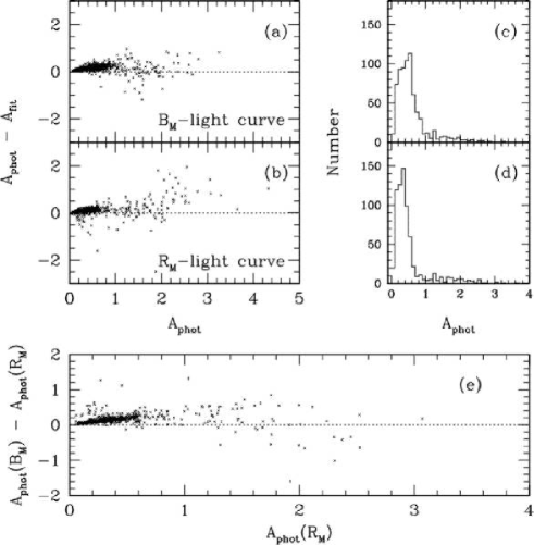
Figure 22: Panel $(a,b)$: The residual $(A_{phot}-A_{fit})$ is plotted against $A_{phot}$. Panel $(c,d)$: Histogram of the amplitude is reported for $B_{M}$ ($c$) and $R_{M}$ ($d$) magnitudes. Panel $(e)$: Difference between amplitude from $R_{M}$- and $B_{M}$-light curves. Only stars with $flag(2)<3$ are shown.