Coronal Evolution of the Sun in Time: High-Resolution X-Ray Spectroscopy of Solar Analogs with Different Ages

Abstract

We investigate the long-term evolution of X-ray coronae of solar analogs based on high-resolution X-ray spectroscopy and photometry with XMM-Newton. Six nearby main-sequence G stars with ages between $\approx 0.1$ Gyr and $\approx 1.6$ Gyr and rotation periods between $\approx 1$ d and 12.4 d have been observed. We use the X-ray spectra to derive coronal element abundances of C, N, O, Ne, Mg, Si, S, and Fe and the coronal emission measure distribution (EMD). We find that the abundances change from an inverse-First Ionization Potential (FIP) distribution in stars with ages around 0.1 Gyr to a solar-type FIP distribution in stars at ages of 0.3 Gyr and beyond. This transformation is coincident with a steep decline of non-thermal radio emission. The results are in qualitative agreement with a simple model in which the stream of electrons in magnetic fields suppresses diffusion of low-FIP ions from the chromosphere into the corona. The coronal emission measure distributions show shapes characterized by power-laws on each side of the EMD peak. The latter shifts from temperatures of about 10 MK in the most rapidly rotating, young stars to temperatures around 4 MK in the oldest target considered here. The power-law index on the cooler side of the EMD exceeds expected slopes for static loops, with typical values being 1.5–3. We interpret this slope with a model in which the coronal emission is due to a superposition of stochastically occurring flares, with an occurrence rate that is distributed in radiated energy $E$ as a power-law, $dN/dE\propto E^{-\alpha}$, as previously found for solar and stellar flares. We obtain the relevant power-law index $\alpha$ from the slope of the high-temperature tail of the EMD. Our EMDs indicate $\alpha\approx 2.2-2.8$, in excellent agreement with values previously derived from light curves of magnetically active stars. Modulation with time scales reminiscent of flares is found in the light curves of all our targets. Several strong flares are also observed. We use our $\alpha$ values to simulate light curves and compare them with the observed light curves. We thus derive the range of flare energies required to explain the light-curve modulation. More active stars require a larger range of flare energies than less active stars within the framework of this simplistic model. In an overall scenario, we propose that flaring activity plays a larger role in more active stars. In this model, the higher flare rate is responsible both for the higher average coronal temperature and the high coronal X-ray luminosity, two parameters that are indeed found to be correlated.

1. Introduction

The solar magnetic field has steadily declined during the Sun’s evolution on the main sequence. Studies of stellar clusters and individual field stars with approximately known ages have shown that the principal parameter determining magnetic activity on a star is its spin rate which, together with convection, controls the operation of the internal magnetic dynamo. As a star spins down due to angular momentum loss via a magnetized stellar wind, its dynamo action weakens, thus continuously reducing magnetic activity expressed in the outer stellar atmosphere. The spin-down history of a solar-like star has been studied in detail by using open-cluster samples (e.g., Bouvier 1990; Soderblom et al. 1993) and accompanying theoretical calculations (e.g., Pinsonneault et al. 1989; MacGregor & Brenner 1991). For a given main-sequence stellar mass in the spectral domain of G and K stars, the rotation period is a rather well-defined function of the star’s age if the latter exceeds a few 100 Myr, regardless of the initial Zero-Age Main-Sequence (ZAMS) rotation rate. For near-ZAMS stars, in contrast, the rotation rate depends on the pre-main sequence evolution and may range between rather modest values (rotation periods $P$ of several days) and rates of the so-called ultra-fast rotators (periods of $\lesssim 1$ d), regardless of the precise stellar age. This spread in rotation rate is well illustrated by stellar cluster samples, such as the Pleiades, in which G and K stars are still close to the ZAMS (Soderblom et al., 1993; Stauffer et al., 1994).

Magnetic activity expresses itself in the outer stellar atmospheres through various phenomena such as dark magnetic spots, bright chromospheric plages, chromospheric emission lines, and coronal radio and X-ray emissions. The coronal emissions display the largest range of variation in response to the surface magnetic activity level. Whereas starspots may cover a few percent of the photosphere of the most active solar analogs, thus producing a photometric wave with a modulation depth of a few percent at best, the range of X-ray luminosity $L_{X}$ in a solar analog spans at least three orders of magnitude between spun-down inactive examples such as the Sun or $\beta$ Hyi (with $L_{X}$ between a few times $10^{26}$ erg s^-1 and a few times $10^{27}$ erg s^-1) and rapid rotators at the “saturation level” ($L_{X}\approx 10^{-3}L_{\rm bol}\approx[2-4]\times 10^{30}$ erg s^-1 for a solar-mass star; Maggio et al. 1987; Güdel et al. 1997a). Even the magnetic cycle of the Sun induces an X-ray luminosity variation over one order of magnitude (Micela & Marino, 2003). Such systematic cyclic or semi-cyclic variations in turn limit the accuracy with which we can attribute “characteristic” X-ray luminosity levels to stars of a given age if other solar analogs are subject to similar magnetic cycles in X-rays, as seems to be the case (Dorren & Guinan, 1994; Dorren et al., 1995).

Short-wavelength ultraviolet and X-ray emissions of a star like the Sun not only serve as a valuable diagnostic to study stellar spin-down and the operation of the internal dynamo, they are also pivotal for the evolution of the outer atmospheres of planets, in particular the photochemistry in the early atmospheres of Earth-like planets (Canuto et al., 1982; Ribas et al., 2005). Motivated by the interest in understanding the Sun’s and our solar system’s past, we have been studying the “Sun in Time” from the early evolutionary stages on the ZAMS to the terminal stage on the main sequence, at ages of 5-10 Gyr. This study encompasses various wavelength regimes, including radio (Güdel & Gaidos, 2001), optical and ultraviolet (Dorren & Guinan, 1994; Guinan et al., 2003), and X-ray wavelengths (Dorren et al., 1995; Güdel et al., 1997a, 1998b). The latter two studies comprise a detailed description of various aspects of the X-ray emission of a solar analog during its main-sequence evolution, based on low-resolution X-ray spectroscopic data from the ROSAT and ASCA satellites. Among the principal findings of that work was a clear trend of decreasing coronal electron temperatures as a solar analog ages, following the decrease in overall X-ray luminosity from ages of $\approx 0.1$ Gyr all the way to ages of nearly 10 Gyr. The authors speculated that the decreasing heating efficiency is due to a decreasing level of coronal flaring owing to a smaller filling factor in older stars. In this picture, the flare rate is responsible both for bringing dense material into the corona and heating it to high temperatures, analogous to the behavior of individual flares observed on the Sun. A large flare rate in younger stars with a higher magnetic filling factor could thus produce X-ray coronae that are more luminous and at the same time are hotter. A larger filling factor is, however, not necessarily needed to make the corona more luminous or hotter, as we will discuss in this paper.

The new generation of X-ray observatories, XMM-Newton and Chandra, offers entirely new access to stellar coronal physics by providing high-resolution X-ray spectroscopy with considerable sensitivity. Apart from more detailed studies of the thermal stratification, they also allow us to derive the coronal abundances of individual elements and to measure electron densities. Both parameters are important for our understanding of the physical processes in stellar coronae. It is now well established that coronae of magnetically active stars show various anomalies in their composition, in particular an overall depletion of metals (e.g., Drake et al. 1994; White et al. 1994) and a relative underabundance of elements with a low ($<10$ eV) First Ionization Potential (FIP) compared to elements with a high ($>10$ eV) FIP (e.g., Brinkman et al. 2001; Güdel et al. 2001; Drake et al. 2001). In the inactive Sun, in contrast, element abundances are arranged according to the so-called FIP-effect, with low-FIP elements being overabundant in the corona relative to their photospheric values and relative to the higher-FIP elements (Meyer, 1985a, b; Feldman, 1992). Similar trends have been noted in inactive stellar coronae (Laming et al., 1996; Drake et al., 1997; Güdel et al., 2002). Because the elemental composition and the element fractionation ultimately derive from the photospheric gas and the physical processes heating it and transporting it to coronal heights, they may be important tracers for the coronal heating mechanism. For example, it has been suggested that the Ne enrichment seen in active stars may be related to increased levels of flaring (Brinkman et al., 2001).

This paper presents a study of six solar analogs at young and intermediate ages observed with the instruments onboard XMM-Newton. The stars range from near-ZAMS ages (0.1 Gyr) to ages between approximately 1–2 Gyr when the rotation period has increased to about 12 days. Together with the Sun, they cover almost the entire path of coronal main-sequence evolution. The present paper is in many ways a follow-up and continuation of the work presented by Güdel et al. (1997a).

Our work emphasizes the similarity of stellar mass, surface gravities and internal structure, i.e., we confine this study to the main sequence and treat rotation (or equivalently, age) as our principal free parameter. In a complementary study, Scelsi et al. (2005) investigate three G-type stars, all at very high activity levels but at largely differing evolutionary stages and with different internal structure and surface gravities, including the young main-sequence star EK Dra, a pre-main sequence (weak-lined T Tau) star, and the evolved Hertzsprung-gap giant 31 Com. They find very similar emission measure distributions in the latter two active stars, regardless of the differences in their fundamental parameters.

The outline of our presentation is as follows. In Sect. 2 and 3 we discuss our targets, the observations, and the principal procedures of the data reduction, respectively. Special attention has been paid to the analysis and interpretation of the spectroscopic data in order to recognize the principal potential and the limitations of the spectral inversion, i.e., the derivation of emission measure distributions and the element abundances. In Sect. 4 we describe the spectra of the six targets. We discuss our methods in Sect. 5. Sect. 6 presents our results, while we discuss various features and models in Sect. 7. Finally, Sect. 8 contains our conclusions.

2. Targets

2.1. General Properties

XMM-Newton data of six young and intermediate-age solar analog stars have been analyzed. The stars are all of early-to-mid spectral type G on the main sequence. Their ages range from approximately 0.1 Gyr for 47 Cas B and EK Dra to $\approx 1.6$ Gyr for $\beta$ Com. These ages have been determined using various proxies such as rotation periods (for the older targets), or memberships in moving groups of known ages (for the younger targets). We have selected these targets because they have been studied in much detail before (e.g., Dorren & Guinan 1994), have well-measured fundamental parameters, and are well-behaved representatives of their age class. A detailed summary and discussion is given in Dorren & Guinan (1994) and Güdel et al. (1997a). The distances quoted are derived from the Hipparcos parallaxes (Perryman et al., 1997), and the rotation periods have been measured photometrically. The general properties of the stars are listed in Table 1, where they are also compared with solar values. The X-ray luminosities $L_{X}$ given there refer to measurements from ROSAT photometry in the 0.1–2.4 keV band (Güdel et al., 1997a, 1998a), and to the spectral modeling discussed in the present paper, also for the 0.1–2.4 keV band, and additionally for the 0.1–10 keV band. For the X-ray luminosity of the Sun, we use a representative value of $\log L_{X}=27.3$ as in Güdel et al. (1997a). This value is in agreement with the $L_{X}$ of $\alpha$ Cen determined by Raassen et al. (2003), $L_{X}=1.6\times 10^{27}$ erg s^-1. A steady decline of $L_{X}$ with increasing age and increasing rotation period $P$ is evident.

The most active target, 47 Cas B, is the fainter component in the 47 Cas binary system. It has not been characterized optically as it has been individually detected only by radio methods (Güdel et al., 1998b) and indirectly from Hipparcos measurements as a companion to the optically bright F0 V star 47 Cas = HR 581 = HD 12230. The radio position is clearly offset from the position of the F0 star. It is, furthermore, very unlikely that early F stars display luminous and spectrally hard X-ray emission (Panzera et al., 1999). On the other hand, all characteristics of the X-ray detection fit well to an early G-type star with an age similar to that of the Pleiades. In particular, the X-ray luminosity corresponds to the saturation level of an early G star ($L_{X}\approx 10^{-3}L_{\rm bol}$, Vilhu 1984), thus excluding a corona of a later-type star as its origin.

A saturated corona requires, for a G star, a rotation period smaller than that of EK Dra. A periodic signal with a period of $\approx 1$ day was reported from the ROSAT All-Sky Survey observations, and was attributed to stellar rotation (Güdel et al., 1995). This period also coincides with the rotation period of the fastest early-G type rotators in the Pleiades (Soderblom et al., 1993). We refer the reader to the detailed discussion in Güdel et al. (1995) and Güdel et al. (1998b). We tried to quantify the maximum contribution of the F0 star to the X-ray luminosity of the 47 Cas system. ROSAT studies of the Pleiades (Stauffer et al., 1994; Micela et al., 1996, 1999) found only few stars with spectral type A7-F3 that have $\log L_{X}>29.4$ (i.e., more than 10% of the $L_{X}$ of 47 Cas), and all of them have known late-type companions, which are likely to be the sources of the high X-ray luminosity (Mermilliod et al., 1992). In addition, the typical X-ray spectrum of F-type stars in the Pleiades is softer than that of G-type stars (Gagné et al., 1995), so we expect the F primary to provide even less flux from hot plasma. In summary, we thus expect the F0 star to contribute less than 10% to the total detected X-ray flux of the 47 Cas system. We therefore add this target to our list of G-type stars, being the only likely solar analog that is accessible to high-resolution X-ray spectroscopy and that is more active than EK Dra, in fact reaching the saturation level.

2.2. Photospheric Composition

When measuring coronal abundances, $A$, of elements, a principal problem is to what standard set of abundances the results should refer to. Often, stellar coronal abundances are cited with respect to the solar photospheric composition. But because the stellar coronal plasma ultimately originates in the respective stellar photosphere, coronal abundances may reflect the composition of the latter, and abundance “anomalies” may simply be due to a non-solar composition of the stellar photospheric material. Fortunately, the photospheric abundances of most of our objects have been measured. The reported photospheric abundances of our sample of stars (except 47 Cas) are given in Table Coronal Evolution of the Sun in Time: High-Resolution X-Ray Spectroscopy of Solar Analogs with Different Ages. The entries refer to individual measurements or to catalogs compiled from previous studies.

As one sees from this literature survey, almost all Fe abundances reported for our targets are compatible with solar photospheric values. Moreover, several measurements for other elements exist, including high-FIP elements such as C, N, and O, and again most of the reports are compatible with solar abundances. We find a trend for super-solar abundances in $\beta$ Com, by perhaps 10–20%. Nevertheless, the photospheric-abundance tabulations for our targets are incomplete and the given measurements scatter, making it impossible to reliably express our coronal abundances relative to the respective photospheric values. However, the above summary makes it clear that our targets (except for 47 Cas) must show a near-solar composition, and we therefore adopt the solar photospheric abundances as the reference composition throughout the paper. As for 47 Cas, to our knowledge no photospheric abundances of the brighter F star in the system have been reported. However, this system is young and is a member of the Local Association (Güdel et al., 1998b), for which we can reasonably assume near-solar abundances, similar to EK Dra, which is also a member of the Local Association.

3. Observations and Data Reduction

3.1. Observations

Our target stars were observed with the Reflection Grating Spectrometers (RGS, den Herder et al. 2001) and the European Photon Imaging Cameras (EPIC, Strüder et al. 2001; Turner et al. 2001) onboard XMM-Newton (Jansen et al., 2001). The RGS are suited for high-resolution spectroscopy in the wavelength range between 6–38 Å, with a resolution of $\Delta\lambda\approx 60-76~{}$mÅ, hence a resolving power of $\lambda/\Delta\lambda\approx 100-500$. The EPICs observe between $\approx$ 0.15–15 keV, providing a moderate energy resolution of approximately $E/\Delta E=20-50$.

We provide a detailed log of the observations in Table 3.

3.2. Data Reduction

The data were reduced using the Science Analysis System (SAS) version 5.4.1. We applied the standard processing performed by the RGS metatask rgsproc and the EPIC MOS task emchain. The PN data (used only for the light curves) were reduced using the PN task epchain.

For the RGS data reduction, we extracted the first-order spectra from a spatial cut including 95% of the cross-dispersion Point Spread Function (PSF) (xpsfincl=95 in rgsproc) and an energy cut including 95% of the pulse-height distribution (pdistincl=95). The background spectra were extracted above and below the source spectra, by excluding 97% of the source cross-dispersion PSF.

For all stars except $\pi^{1}$ UMa, $\chi^{1}$ Ori, and $\beta$ Com the MOS data were taken in the small-window mode. In this mode, only the central $100\times 100$ pixels of the middle CCD are operational, whereas the outer CCDs work in full mode. The small-window mode allows for shorter integration times for the source and thus avoids the brighter sources from becoming piled up. The disadvantage of this mode is, however, that the central window is too small to reliably extract a background region. We therefore selected a source-free region in one of the outer CCDs. The target source itself was extracted from a circle as large as possible in the small window (with a radius of approximately 50^′′).

For $\pi^{1}$ UMa, MOS1 was in full window mode whereas MOS2 was in small-window mode. The exposure time was 5000 s longer in MOS1. Pile-up was studied for both MOS cameras with the SAS epatplot task. This task makes use of the relative ratio of single- and double-pixel events, that deviate in case of pile-up. Since no evidence for pile-up was found for this star, we decided to use MOS1.

For $\chi^{1}$ Ori, MOS1 data were taken in timing mode and MOS2 data in full-window mode. We did not use data taken in timing mode because reliable background subtraction cannot be performed. We found that pile-up was not negligible in the MOS2 data and therefore used an annular extraction region for the source, with inner and outer radius of 80 and 1200 detector pixels (4 and 60 arcsec), respectively, in order to remove the piled-up central part of the PSF.

For $\beta$ Com both MOS1 and MOS2 observed in full window mode. We found that pile-up did not affect this source.

In those cases where the background area was selected in one of the outer CCDs, the background count rates could have been underestimated with respect to the source extraction region due to vignetting. We studied background behavior effects using the eboxdetect SAS task. This task detects all sources in the field of view; these were subsequently cut out from the image. We then quantified the remaining background count rate per unit area as a function of the distance from the center of the field of view, by analyzing the average rates in annuli at different radii. We found a decrease of at most 10% from the image center to the central portions of the outer CCDs, which is negligible when compared to calibration uncertainties, particularly in the light of the high count rates of our sources. The only possible but small influence could be on the data at the highest energies where the source flux drops below the background flux. We therefore decided not to consider spectral data at energies where the background count rate exceeded the source count rate.

We used the rgsrmfgen task for RGS and the rmfgen and arfgen tasks for MOS to generate response and ancillary files appropriate for the specified extraction regions. To avoid bins with very few counts, we grouped the spectral channels: the MOS data were grouped to a minimum of 25 counts per bin, whereas the RGS data were grouped to a minimum of 10 counts per bin. The very weak continuum level in the RGS spectra of $\beta$ Com made this grouping scheme not well suited; instead, we regularly rebinned the entire RGS spectra by a factor of five.

Finally, we studied the agreement between the observed wavelengths of bright emission lines with their tabulated rest wavelengths (stellar radial velocities being negligible); in cases where small systematic offsets due to residual calibration uncertainties of order 10 mÅ were found, we slightly updated the assumed boresight coordinates accordingly and repeated the data reduction.

4. Description of the Spectra

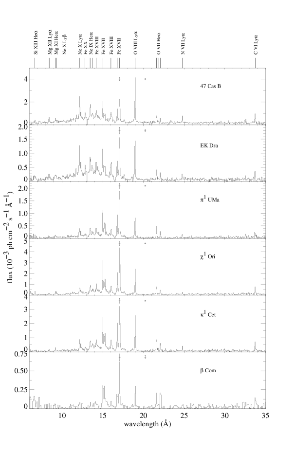
Before quantitatively evaluating the observed spectra, we discuss some general features. Fig. 1 reveals four significantly different types of spectra: i) the most active star, 47 Cas B, shows typical features of a very hot plasma, namely a well-developed bremsstrahlung continuum, lines of Mg xi and xii, and comparatively high flux ratios of O viii $\lambda 18.97$/O vii $\lambda 21.60$, of Ne x $\lambda 12.13$/Ne ix $\lambda 13.45$, and of Fe xviii $\lambda 14.20$/Fe xvii $\lambda 15.01$. ii) The spectrum of EK Dra is significantly cooler, which is in particular evident from the smaller O viii/O vii flux ratio, a more modest continuum level compared to the line strengths, and a marked dominance of the Fe xvii lines. iii) The third group consists of the intermediately active, intermediately old stars $\pi^{1}$ UMa, $\chi^{1}$ Ori, and $\kappa^{1}$ Cet which all show very similar spectra in which the Fe xvii lines are much stronger than those of Fe xviii, and the O viii/O vii flux ratio is further reduced. Note that the maximum formation temperature of Fe xvii is only $\approx 5$ MK. The continuum has become very weak in these spectra. iv) Finally, the spectrum of the least active target, $\beta$ Com, is largely dominated by lines of Fe xvii, and the O viii/O vii flux ratio approaches unity.

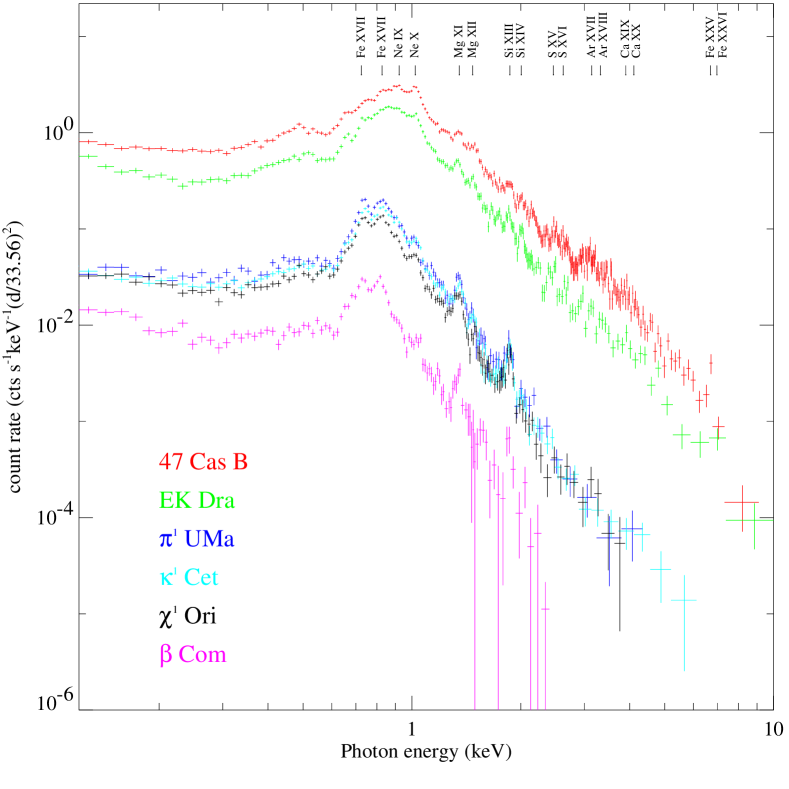
Turning to the EPIC MOS spectra in Fig. 2, further indicators support this picture. In this figure, we have renormalized the MOS spectra so as to represent the stars at a common distance of 33.56 pc, identical to the distance of 47 Cas B. A marked decrease of the overall emission level is seen as the stellar age proceeds from the sample of Pleiades-age stars (47 Cas B, EK Dra) to the older sample. The most active stars show shallower continuum spectra between $\approx 2$ and 10 keV than the less active targets, indicative of the higher overall plasma temperatures of the former. The dominant Fe xvii lines (at 0.826 keV and 0.727 keV) are well developed in the spectra of the less active stars.

5. Data Analysis

Because the novel aspect of our X-ray data is the high spectral resolution of the RGS, allowing us to access individual emission lines from different elements, we used the spectral data from both RGS instruments but used EPIC data only in so far as they contribute additional information not accessible by RGS, such as spectral data at wavelengths shorter than 6 Å. To keep maximum weight in our data analysis on the RGS data, we restricted the more sensitive EPIC spectral data to one of the three cameras. We chose MOS1 or MOS2, because the MOS spectral resolution is superior to that of the pn camera, and the S/N at higher energies balances well with the S/N provided by RGS at lower energies. Also, the cross-calibration between MOS and RGS is better understood (they use the same mirrors). Only for the light curves did we make use of the data of other EPIC cameras as well.

For the analysis of each target, we used the exposure time covered simultaneously by all three detectors. Each light curve except that of $\beta$ Com contained one well-developed flare. In order to avoid systematic bias by any of these flares (i.e., increasing the average $L_{X}$ and possibly also increasing the characteristic coronal temperatures), we eliminated the flare intervals from consideration. We will, however, briefly present and discuss the individual light curves separately in Sect. 6.3. The exposure times remaining for our spectral analysis are listed in Table 3 (last column).

5.1. Spectral Inversion

An observed coronal X-ray spectrum is the superposition of the spectra emitted by various coronal features with different temperatures, volumes, densities, and possibly different composition in terms of chemical elements. The inversion of an observed spectrum to obtain the underlying physical parameters is therefore a highly degenerate problem, with numerous solutions describing essentially the same spectrum.

For our analysis we consider a coronal model with the following, observationally tested assumptions of the physical parameters. First, the plasma is assumed to be in collisional ionization equilibrium, a model that appears to be sufficiently good as long as no very rapid change in the heating rate of the plasma is taking place (Mewe, 1999). We also assume that the coronal plasma is effectively optically thin and that lines with high oscillator strengths are not subject to resonance scattering, an assumption that has been shown to be justified for the stars in our sample (Ness et al., 2003). Furthermore, the density-dependence of the populations of metastable levels is neglected, i.e., the spectrum is computed in the low-density limit. This approximation is supported by the flux ratios in the He-like triplet of O vii in our observations, and it appears to be a reasonable assumption for most coronal plasmas (Ness et al., 2004; Testa et al., 2004).

At this point, then, the observed spectrum is essentially a function of the distribution of optically thin coronal features in volume, temperature, and elemental composition; conventionally, the thermal distribution is described by the differential emission measure distribution (DEM),

$$Q(T)={n_{e}n_{H}dV\over d{\rm ln}T}$$ (1)

where $n_{e}$ and $n_{H}$ are the electron and hydrogen number densities, respectively, and $dV$ is a differential volume element at temperature $T$. The DEM determines the line flux $F_{j}$ of any given emission line $j$ through

$$F_{j}={1\over 4\pi d^{2}}\int A\varphi_{j}(T)Q(T)d{\rm ln}T.$$ (2)

Here, $\varphi_{j}$ is the line power per unit emission measure (“emissivity” henceforth), and $A$ is the abundance of the element emitting the relevant line, with respect to some standard tabulation (such as “solar photospheric abundances”) used for the computation of $\varphi_{j}$.

Non-solar abundances in stellar coronae are now well established (e.g., Brinkman et al. 2001; Drake et al. 2001; Audard et al. 2003a), and we recall that the corona of the Sun itself shows considerable deviations from the photospheric mixture. However, it is also known that the solar coronal abundances vary greatly from feature to feature, some showing a marked FIP bias, with others showing photospheric composition (Feldman, 1992; Laming et al., 1995). Our spectra are - like most existing stellar X-ray spectra - insufficient to characterize abundances at various separate temperatures; therefore, we will assume $T$-independent abundances to at least recognize overall trends in our stellar sample.

The spectral inversion problem is mathematically ill-posed. Statistical scatter due to photon statistics in line fluxes, even if amounting to only a few percent, may introduce considerable scatter in the reconstructed emission measure distribution (Craig & Brown, 1976). We expect a strong amplification of such effects from the uncertainties in the atomic physics parameters (which may amount up to a few tens of percent for the emissivities) and from calibration uncertainties (up to several percent in certain spectral regions).

Therefore, the spectral inversion can essentially be performed in a meaningful way only by constraining the problem suitably, for example by subjecting the reconstruction to smoothness conditions for the resulting, discrete Emission Measure Distribution (EMD), or by iterating the problem using a pre-defined convergence algorithm that reconstructs a preferred, physically meaningful solution (see, e.g., Kaastra et al. 1996a and Güdel et al. 1997b for a discussion of various algorithms with different bias).

We have chosen here to perform the inversion using two widely different algorithms that we briefly summarize as follows:

• Method 1 (M1). We fitted the spectrum using synthetic template spectra calculated for a set of physical parameters; the parameters were varied until the fit was optimized. This method has conventionally been used for low-resolution spectra but also for high-resolution grating spectra, in particular as implemented in the SPEX (Kaastra et al., 1996b) and the XSPEC (Arnaud, 1996) software packages. We, however, modified the conventional approach by including almost exclusively segments of the spectrum that are dominated by bright lines for which comparatively robust atomic physical parameters should be available, together with some nearly line free regions.

• Method 2 (M2). Here, we worked with a list of discrete line fluxes that we extracted from the observed spectrum. If the formation temperatures of these lines cover the range of relevant coronal electron temperatures, then the EMD can be reconstructed by successive approximation, essentially inverting a system of equations like Eq. (2).

We emphasize the complementarity of our two approaches: method 1 uses all tabulated emission lines and their blends within the selected spectral segments, while we confine method 2 to a minimum number of lines, namely the brightest lines available, required to derive meaningful EMDs and the most essential abundances.

Both methods are subject to separate biases. Some of the many lines considered in method 1 may be poorly fitted, owing to discrepancy in the tabulated emissivities. If the latter scatter around their true values, the resulting fit may show reduced systematic errors compared to a fit based on one single line per ionization stage. The individual lines in method 2 may be better described, but their small number makes the inversion process rather sensitive to any systematic uncertainty in any of the line emissivities, and some a priori estimate for blend contribution must be considered. Lines not tabulated in the line-emissivity lists affect both methods, either by altering the measured line flux in method 2 through unrecognized blending, or by adding a continuum-like base level if many weak lines contribute in either of the analysis methods.

A comparison of method 2 with a method using polynomial EMDs to calculate synthetic spectra has previously been presented by Audard et al. (2004) for the extremely active and hot corona of the FK Com-type star YY Men. These authors found that both the reconstructed EMDs and the derived abundances closely agreed for the two methods. Here, we study and compare the results for stars across a large range of activity and coronal temperatures.

To further assess potential sources of systematic error, we applied two different databases to each of the two methods. The spectral models are based on the assumption of coronal ionization equilibrium (CIE). We used the atomic parameters from the MEKAL database in SPEX vers.2.0 (Mewe et al. 1985; Kaastra et al. 1996b) and from the Astrophysical Plasma Emission Code vers.1.3.1 (APEC, Smith et al. 2001) in XSPEC (Arnaud, 1996). The MEKAL emissivities are computed using the ionization balance of Arnaud & Raymond (1992) for Fe and Arnaud & Rothenflug (1985) for the other elements. The APED emissivities (emissivities used in the APEC code) are computed using the ionization balance of Mazzotta et al. (1998).

5.2. Method 1: Synthetic Spectra

Here, we used an approach essentially identical to the one described in Audard et al. (2003a), apart from slightly different wavelength ranges (see below). Because numerous emission lines are poorly described by the spectral line lists in use, we confined our analysis to a restricted number of spectral regions that contain bright lines for which the atomic physics is believed to be relatively well known, and some nearly line-free regions of the spectrum where the continuum dominates. The wavelength ranges of the selected regions are summarized in Table 4. As we decided to put more weight on the data from the RGS with its higher spectral resolution, we used EPIC MOS data only in the wavelength range shortward of 9.35 Å, where the RGS effective area is small and its calibration is less accurate. We thus cut the RGS data shortward of 8.3 Å, so that the data from the RGS and the EPIC instruments overlapped around the Mg xi and Mg xii lines. As mentioned in Section 4, we discarded the high-energy part of the EPIC spectrum where the background flux exceeded the source flux (see Table 4).

The physical model was defined as a combination of 10 optically thin, thermal CIE models, and a photoelectric absorption component. The photoelectric absorption was frozen by defining a fixed interstellar hydrogen column density. The latter ranged between negligible values ($<10^{18}$ cm^-2) for the closer stars and $7\times 10^{18}$ cm^-2 for 47 Cas B. These values are consistent with hydrogen column densities given by Güdel et al. (1997b) and Audard et al. (1999) and with values of the interstellar hydrogen density given by Paresce (1984). However, even the largest values used here were too small to significantly alter our model spectra even at the longest wavelengths in the RGS.

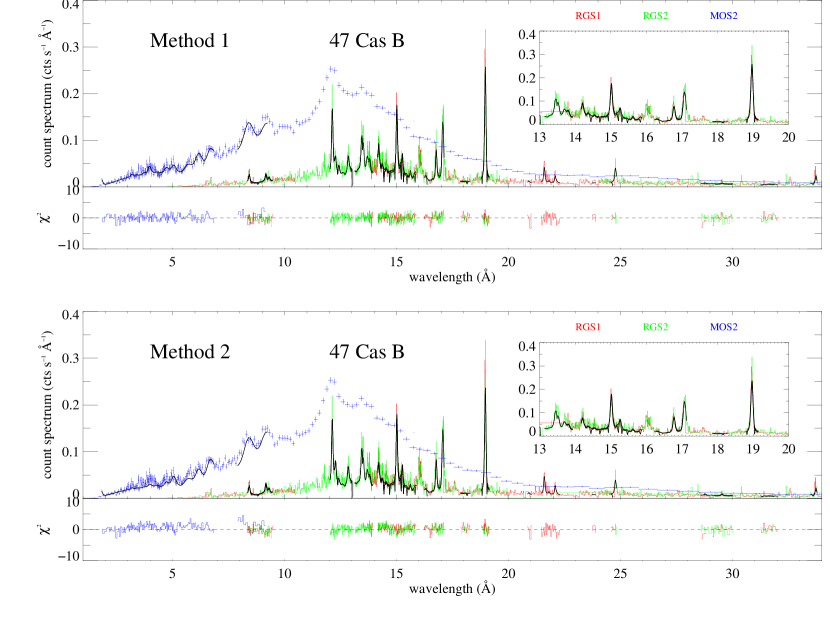
Each of the ten CIE temperatures was confined to within one of ten adjacent temperature intervals of equal width (0.22 dex) in $\log T$; to optimize the multi-temperature fit, given the relatively broad bins, we treat the temperature values as free parameters within the bounds of the respective bin intervals, as well as the associated emission measures. The temperature intervals covered the range from $\log T$=6 to $\log T$=8.2 ($T$ is given in K). The abundances of C, N, O, Ne, Mg, Ar, Si, and S were also used as free parameters. Only the abundances found with the 10-temperature fit were used in a second step for the DEM reconstruction. The Chebychev polynomial DEM code in SPEX, with polynomials of order 6 and 8, was used to describe the DEM that best fitted the given spectrum. An example of a best fit is shown in Fig. 3, which also illustrates the spectral ranges used for this procedure.

5.3. Method 2: Inversion of Line-Flux Lists

5.3.1 EMD Reconstruction

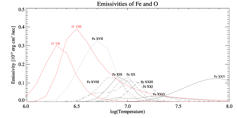
We reconstructed the discrete EMD starting from fluxes of individual lines. In order to obtain an EMD independently of the element abundances, we selected a few well-defined, bright Fe lines from the ionization stages of Fe xvii to Fe xxv (as far as measurable, see Table 5). The Fe xvii-xxiv lines were extracted from the RGS spectrum, whereas the unresolved Fe xxv line triplet was extracted as a single blend system from the MOS spectrum. The emissivities of the Fe xvii-xxiv lines cover the temperature range between 3 MK and 20 MK rather well, and for the more active stars (47 Cas B and EK Dra), Fe xxv constrains the hottest temperatures, up to about 100 MK (Figure 4). In order to obtain information on the cooler part of the EMD in which no Fe lines are detected, we used the flux ratio between the OVIII $\lambda$18.97 and the OVII $\lambda$21.60 resonance lines, which itself is independent of abundances. The lines used for each star are listed in Table 5 and Table 6, together with their measured luminosities.

To avoid cross-talk with the abundance determination, we selected only lines of Fe that are not strongly blended with lines of other elements (with the exception of Fe xix, see below; the Fe xvii lines at 17Å were not used because they are partly obscured by one of the RGS CCD gaps). Nevertheless, our line features usually still contain a number of weaker blends from various Fe ions. We thus considered all Fe blending lines close to the principal line as being part of our Fe feature and we therefore computed new $T$-dependent emissivity curves for each such Fe blend system. The line feature, composed of all Fe lines in the chosen wavelength range, was thus subsequently treated like a single emission line. In the RGS spectrum, all tabulated blending Fe lines within $\pm 0.06$ Å (one FWHM on each side) of the wavelength of the principal line were considered. In the MOS spectrum, the range was chosen to be $\pm 0.15$ Å.

In a first step, we extracted the fluxes of the relevant Fe lines and of the O viii $\lambda 18.97$ and O vii $\lambda 21.60$ resonance lines from the spectrum. This can be problematic, because the lines have broad wings due to the RGS PSF, and the determination of the underlying continuum is difficult. Moreover, in some cases, blends with lines from different elements may still be present, in particular in the case of the brighter lines of Fe xix that are blended with Ne ix lines. While the effect of these blends cannot be assessed a priori without knowledge of the thermal structure and the abundances, we can obtain useful approximations as follows. Because most ions are represented by several different emission lines, and the continuum can be interpolated from values obtained in nearly line-free regions of the spectrum, a good approximation of the contaminating blends and of the baseline continuum level in fact comes from the fit we derived in method 1. We emphasize that we have not used that model to derive parameters, but only to obtain an approximate description of the baseline spectral flux distribution on which the line fluxes of interest are superimposed. The latter being the fluxes of Fe lines, we set the Fe abundances in the best-fit model from method 1 to zero, retaining only the emission lines and the continuum from all other elements. We note that neglecting Fe does slightly change the continuum as well, but the influence is on the order of a few percent in the temperature and wavelength range of interest if solar abundances are assumed. Anticipating sub-solar abundances in active stars with a strong continuum as reported in the previous literature, the contribution of Fe to the continuum will be even smaller. The errors thus introduced into the line-flux extraction are negligible. An equivalent procedure was then also applied to extract the O viii and O vii line fluxes, although in these cases, blending was not significant.

Before extracting individual lines, we need to make sure that the baseline continuum level has been correctly fitted individually in each spectrum. We checked the relevant fits in a nearly line-free region of the RGS spectrum, namely immediately shortward and longward of the O viii $\lambda 18.97$ resonance line by multiplying the EM by a suitable factor. We found that an optimization of the continuum level in these wavelength regions required a change in flux of only a few percent. It is not clear whether this is due to slight cross-calibration problems or to some bias in the fit. Such bias may be introduced by the fact that the MOS spectral portion, determining mostly the hotter part of the DEM, has a relatively high S/N ratio which may lead to some over- or underestimation of the hot EM. Because the latter produces continuum at all wavelengths, a slight offset could also affect the soft part of the RGS spectrum. Given the small magnitude of the effect, we are unable to ascribe such an offset either to (possibly wavelength-dependent) cross-calibration problems or to fit bias as described above. Our final results indicate that any such effect is of minor consequence and does not need to be considered for the overall fit in method 1. For the extraction of line fluxes in method 2, however, we need to optimize the continuum level so that the line flux can be properly defined as an excess above this baseline level.

In a similar manner, we extracted the Fe xxv $\lambda 1.85$ line by first optimizing the nearby continuum level starting from the overall best-fit provided by method 1. Again, the continuum renormalization required for this procedure was at most a few percent in the spectral region of interest.

To actually extract the line fluxes, we added $\delta$ function lines to the model, located at the theoretical wavelengths of the principal lines in the blends under consideration, and convolved them with the instrument response. The line fluxes were then obtained by fitting the amplitudes of the $\delta$ functions to the observed lines and the adjacent narrow wavelength ranges. If the wings of two Fe lines overlapped significantly, we fitted two $\delta$ functions simultaneously. Note that the fluxes thus derived may be different for APEC and MEKAL because of slightly different atomic physics, fit parameters, and blend contributions.

The obtained Fe, O viii and O vii line fluxes were converted to luminosities as presented in Table 5 and 6 for MEKAL and APEC emissivities, respectively, based on Hipparcos distances as quoted in Table 1. They were then used to reconstruct the EMD, as follows:

A first, smooth estimate of the EMD was derived from the emissivities at the maximum line formation temperature $T_{m}$ of each Fe line. The emissivities are based on solar abundances as given by Anders & Grevesse (1989). Our EMD was defined on a grid with a grid point separation of $\Delta\log T$=0.1 dex in the range between $\log T=5.5-8$ for SPEX ($T$ in K) (APEC: $\log T=5.7-8$) for the more active stars 47 Cas B and EK Dra, and in the range between $\log T=5.5-7.1$ (APEC: $\log T=5.7-7.1$) for the less active stars $\chi^{1}$ Ori, $\kappa^{1}$ Cet and $\beta$ Com. For $\pi^{1}$ UMa, the EMD was defined in the range between $\log T=5.5-7.3$ (APEC: $\log T=5.7-7.3$). (The different low-temperature limits reflect the different availability of emissivities in the different codes, but we note that the range of $\log T=5.5-5.7$ is irrelevant for any line we use for the EMD reconstruction, and it is also not important for the emissivities of any lines of other elements analyzed here.) As a starting condition, the EMD was extrapolated to temperatures cooler than $T_{m}$ of Fe xvii ($\log T=6.7$) by using a slope of 2, and to temperatures higher than $T_{m}$ of the hottest Fe ion in use (Fe xxv, $\log T=7.9$ for 47 Cas and EK Dra, Fe xix, $\log T=6.9$ for $\beta$ Com, and Fe xxi, $\log T=7.0$ for the other stars) by using a slope of –2. These extrapolations were performed to the limits of the respective temperature ranges as defined above. These starting conditions were suggested by the slopes of the initial EMDs defined by the EM values at the different $T_{m}$. Also, we subsequently found that the low-$T$ slope converges to values around 2 even if the starting slope was largely different (see Sect. 7.3). For each line, the flux $F_{C}$ predicted from the initial EMD was calculated according to the following equation:

$$F_{C}(x)=\sum_{i}{\rm EM}(i)\cdot\varphi(x,i)$$ (3)

where the sum is over the temperature bins $i$; EM$(i)$ is the emission measure in the $i$th temperature bin, and $\varphi(x,i)$ is the emissivity of the given line $x$ at this grid point. The calculated fluxes were then compared with the measured fluxes, $F(x)$. The EM in each bin was iteratively corrected using the algorithm described by Withbroe (1975):

$${\rm EM}^{n+1}(i)={\rm EM}^{n}(i)\cdot\frac{\sum_{x}\frac{F(x)}{F_{C}(x)}\cdot\varphi(x,i)+\frac{R_{C}}{R}\cdot\varphi(\mathrm{O\,VII},i)}{\sum_{x}\varphi(x,i)+\varphi(\mathrm{O\,VII},i)}$$ (4)

where $i$ is the index of the temperature bins and $n$ is the iteration number. The last term in the numerator and denominator was added to also obtain convergence of the line-flux ratio between O viii and O vii, where we have used the measured ($R$) and the predicted ($R_{C}$) flux ratio. The EMD was then iterated until we reached a pre-set convergence criterion.

In the presence of considerable systematic uncertainties in the modeling, a reasonable convergence criterion should be set, although its statistical meaning may be marginal. A straightforward goal is to achieve convergence in such a way that on average the squared deviation between model and fit for a line flux is equal to the variance of the same line flux. This leads to a reduced-$\chi^{2}$-like expression,

$$\psi^{2}=\frac{1}{N_{x}+1}\left(\sum_{x}\left[\frac{(F[x]-F_{C}[x])^{2}}{(\sigma[x])^{2}}\right]+\frac{(R-R_{C})^{2}}{(\sigma_{R})^{2}}\right)$$ (5)

where the last term relates to the O viii/O vii flux ratio. Here, $N_{x}$ is the number of lines used, and $\sigma(x)$ is the error assigned to the measured line flux, which comprises the error from the finite photon statistics and an assumed systematic uncertainty from the atomic physics (see Sect. 5.3.3). Similarly, $\sigma_{R}$ is the derived error in the O viii/O vii flux ratio. We iterated until this expression reached a value of unity, or if this did not occur, until it no longer significantly decreased. We would like to mention that the fit parameters, i.e., the EMs per bin, are not independent of each other owing to the broad emissivity curves of each line; given the large systematic uncertainties in the line fluxes, we feel that a more detailed convergence criterion is not warranted. Our main goal is to stop the iteration at a reasonable level to avoid over-interpretation of superficial features in the EMD that may arise from iterating too deeply - see our discussion in Sect. 6.1.

At this point, then, we have found an EMD from fluxes of the single element Fe, under the assumption of solar metallicity as used for the tabulated emissivities, and from a ratio of O line-fluxes. Therefore, there still remains a normalization factor for the EMD and the absolute level of the Fe abundance to be determined (see Sect. 5.3.2). We will use the observed continuum level to fix the EMD normalization and, at the same time, the absolute Fe abundance, as explained in the following.

5.3.2 Abundances

To determine the abundances of the elements, we extracted all lines of interest (see Tables 5 and 6) in a similar manner as we extracted the Fe and O lines before. Here, however we used the EMD constructed from our Fe and O line fluxes in order to describe the continuum, instead of the 10-$T$ model. This EMD is known only up to a normalization constant depending on the absolute Fe abundance, which we derived as follows: we constructed a set of spectra from the calculated EMD with different Fe abundances such that the product of the Fe abundance and the EM$(T)$ is constant for any $T$, still using the approximate abundances of the other elements from method 1 to estimate the contributions from blends and to obtain a more accurate description of the continuum. From the spectrum that best fitted the nearly line-free regions long- and shortward of the O viii Ly$\alpha$ line at 18.97 Å , we obtained the absolute Fe abundance. We then extracted the line fluxes of all interesting elements using $\delta$-line models, as described before. Note that the line fluxes of Mg, Si, S, and, if available, Fe xxv, were extracted from the MOS spectra while all other lines were extracted from the RGS spectra. As done for the RGS spectra before, we adjusted the model continuum to the observation in the line-free regions of the MOS instrument at high energies, before the line-flux measurement.

The predicted line fluxes of these elements (see Table 5 and 6) were then calculated from the EMD, using their catalogued emissivities, which were again based on solar photospheric abundances. The ratios between the predicted and the measured fluxes provided the abundances relative to Fe, $A/A(\rm Fe)$, with respect to the corresponding solar ratios. In some cases, we measured the fluxes of more than one line for a single element. In these cases, we calculated the abundance for each line and computed averages, using $1/\sigma_{A}^{2}$ as weights, where $\sigma_{A}$ is the error in the abundance (see Sect. 5.3.3). We implicitly assumed here that the abundance of an element is the same at all temperatures, an assumption that is not necessarily supported from solar observations (Jordan et al., 1998). The data quality at hand does not allow for further discrimination, however.

Finally, we once more iterated the adjustment of the continuum level to obtain the absolute Fe abundance, as described above, now using the abundances determined from our procedure. The updated values closely agreed with the previously obtained Fe abundances. The error of the absolute Fe abundance was derived by varying it around its best fit value and requiring that the continuum fit be acceptable within one sigma. The final abundance values we report in this paper refer to the solar photospheric abundances given by Anders & Grevesse (1989), except for Fe for which we adopt the value given by Grevesse & Sauval (1999).

5.3.3 Errors

Errors arise from different sources. First, they are due to uncertainties in the atomic databases; these are not easily quantifiable, but are likely to be in the range of several percent to perhaps 20%, depending on the line under consideration. For method 2, we chose mostly bright, well-studied lines, and for the sake of definition we have assumed systematic uncertainties of 10% for each line. Statistical errors also arise from the fit of the $\delta$-line model used to extract the line flux; these essentially originate from photon statistics. For each line flux, these two errors were summed in quadrature, and we call them line-errors $\sigma$.

The errors in the EMD were estimated by statistically varying the fluxes of the line blends according to their $\sigma$, and repeating the EMD reconstruction for 19 different, perturbed line-flux lists. We thus derived formal upper and lower 1-sigma ranges of the EMD solutions by using standard formulae from Gaussian statistics, although we mention that the various solutions are not necessarily normally-distributed in $\log$ EM at any given temperature. The standard deviations thus derived, however, provide a well-defined characteristic width of the distribution, and we verified that the ranges containing 68% of the solutions and the 1-sigma ranges are very similar. Because the EM values scatter considerably in any temperature bin, we performed the statistics using logarithms of the EMs in each temperature bin in order to avoid the average being biased by one or a few large values. We extended the error analysis to include up to 100 perturbed line lists but the error ranges did not significantly change. We caution that the EMD slopes on both sides of the peak temperature could be slightly dependent on the initial EMD guess, where we assume a slope of $\pm 2$ (see Sect. 5.3.1). We study the EMD results starting from different initial conditions for the slopes in Sect. 7.3. The final EMD slopes converged to similar values. These effects are not taken into account in the EMD errors reported here. We note that these errors are only given as an indicator for the uncertainty in the EMD, but they are not explicitly used further in our error analysis.

The error of the abundance $A$ is proportional to the line-error, $\sigma_{A}=A\cdot\sigma(x)/F(x)$. If the abundance is a weighted average, then the final error is the larger of i) $(\sum 1/\sigma_{A}^{2})^{-1/2}$ and ii) the error of the weighted means of all abundance values. Moreover, there is an error in the abundances arising from the variation in the 20 different EMD reconstructions: for each of these reconstructions, we found slightly different abundances with new errors. We defined the error from this variation as the larger of i) the average error found in each reconstruction, and ii) the standard deviation of the twenty abundance values per element. We note, however, that we adopted the abundance derived from the best-fit solution, with no perturbation applied.

Finally, the error in the adjustment of the continuum (required to determine the line fluxes, Sect. 5.3.2) also affects the abundance errors. As our final error for a given abundance, we summed in quadrature the error related to the line-error (or the average if multiple lines were used, as defined above), the error arising from the variation of the EMD, and the error from the continuum adjustment. We emphasize, however, that this procedure can provide no more than a simulated estimate of realistic errors. The unknown systematic deviations in the atomic physics parameters prevent us from obtaining better estimates.

6. Results

6.1. Emission Measure Distributions

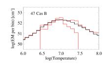
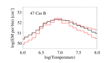
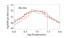
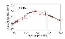
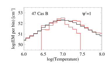
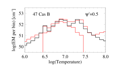
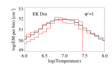
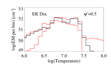
The EMDs derived from the two different methods are shown in Figure 5. In the left column, EMDs from method 1 using SPEX in combination with a fit based on Chebychev polynomials of degree 6 and, where possible, 8 are plotted. The middle and the right columns show EMDs reconstructed with our method 2, based on MEKAL and APEC emissivities, respectively. In the middle and right columns, the black histograms illustrate the best-fit EMDs while the red histograms mark the $1\sigma$ range at each temperature, derived from the perturbed flux lists. As the best-fit EMDs are derived from unperturbed fluxes, and they are not equal to the mean EMDs derived from the perturbed flux lists, these ranges of variation do not need to be symmetrically arranged around the best-fit solutions. In some cases (EK Dra and 47 Cas B), the lower error ranges drop rapidly to very low values at certain temperatures. Although this is a consequence of the increasing uncertainty in the EMD at the lowest and the highest temperatures, we note that the error ranges are given on a logarithmic scale; once the ranges becomes large, the precise level of the lower bound is of little importance.

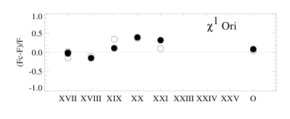
For method 2 the quality of the EMD can be measured by comparing the predicted and the observed line fluxes. The final agreement between predicted and observed line fluxes is illustrated in Fig. 6, where we show the fractional deviation of the predicted line fluxes from the observed values, $(F_{C}-F)/F$ for Fe and O viii/O vii flux ratio. Most line fluxes agree within 10–20%, with the larger deviations mainly relating to the weakest lines, i.e., the lines formed at high temperatures in the least active stars (e.g., Fe xx for $\pi^{1}$ UMa).

The EMDs derived from the different methods show rather similar characteristics. We see that the temperature where the EMD peaks decreases toward older, less active stars, namely from about 10 MK for 47 Cas B and EK Dra to 5 MK for $\pi^{1}$ UMa, $\chi^{1}$ Ori and $\kappa^{1}$ Cet, and to $\lesssim$4 MK for our oldest target, $\beta$ Com. Characteristic values for the Sun are 1–3 MK, depending on the phase of its activity cycle (Peres et al., 2000). The average temperatures derived from method 2, $\log\bar{T}$, are listed in Table 7. To obtain these values, we calculated the mean of $\log T$, using the EMs in each bin as weights. Also given are the lower and upper threshold temperatures that comprise 90% of the total EM (on each side of the EMD peak).

With method 2, we generally obtain a smoother and flatter EMD than with method 1 and the Chebychev polynomial approximation. At temperatures above $\log T\approx 7.5$, the EMD is not well constrained. This is obvious for the cooler coronae which do not provide any useful spectral lines at those temperatures, and we therefore did not extend our DEM analysis to this range. Considerable scatter is still also found for the EMDs of 47 Cas B and EK Dra, despite the availability of Fe xxiii-Fe xxv lines. The reason resides in the fact that Fe xxiii and Fe xxiv show very faint lines, and Fe xxv is the only blend complex that covers the temperatures above $\log T\approx 7.5$. In the more active stars, the EMDs from method 1 seem to be composed of two peaks at about 6 and 20 MK, well separated by a local minimum. Also, in most EMDs derived from method 1, we find a deep decrease in the EM below about $\log T\approx 6.2$, combined with a local EM peak around $\log T=6.0$. Both features become stronger if higher polynomial degrees are used.

Several effects may contribute to this: First, a large range of solutions may in fact be compatible with the spectra, given that the spectral inversion is ill-conditioned, in particular in temperature regions where few constraints are available. Second, the fit of method 1 iterates to minimum $\chi^{2}$, which considers only the Poissonian errors in the count spectrum and which may introduce EMD features of little relevance given the systematic uncertainties in the atomic physics, while method 2 has been terminated according to $\psi^{2}$ (see Eq. 5), which approximately considers the atomic physics uncertainties as well. Third, method 1 uses many lines that may introduce uncertainty to the spectral fit, while the result of method 2 almost uniquely relies on the O viii/O vii flux ratio for the coolest portion of the EMD. And finally, method 1 imposes polynomial constraints on the solution, which favours the appearance of peaks and valleys in the EMD, while method 2 starts with a smooth EMD that is changed only in so far as the spectrum requires. For example, if a line requires excess EM due to an underestimation of its emissivity at a given temperature, then the reconstruction process may compensate by lowering the EM at adjacent temperatures as dictated by lines dominating there. To test this hypothesis, we iterated method 2 excessively, to $\psi^{2}=0.5$. As the two examples in Fig. 7 show, very similar features also evolve in these examples. The low-temperature slopes appear to become partly steeper as well.

We also note that the amplitudes of the oscillations are compatible with the error ranges from perturbing the line-flux lists used in method 2 (cf. Fig. 5). It is conceivable that the oscillations found after a deep iteration of method 2 correspond to those seen in method 1 although this cannot be explicitly proven, given the largely different approaches. However, the magnitudes of the oscillations appear to be similar. It is also possible that the oscillations are present in the stellar EMD; we cannot reliably discriminate between this hypothesis and a numerical effect as long as we include statistical errors and assume the presence of systematic uncertainties of the magnitude adopted here (see Sect. 5.3.3).

In contrast, the abundance ratios turn out to be robust, with no significant change when deeper iterations are applied. In fact, the synthesized spectra for the two cases are very similar, i.e., the two EMDs represent the spectra almost equally well. Comparing the synthesized spectrum with the observations in the wavelength intervals illustrated in Fig. 3, we find, for 47 Cas B, a reduced $\chi^{2}$, $\chi^{2}_{\rm red}=1.28$ (for 1091 d.o.f) for the deeper integration and $\chi^{2}_{\rm red}=1.37$ (for 1091 d.o.f) for our standard convergence criterion. Although at first sight this difference appears significant, the important line features and the continuum in the RGS are fitted well in both cases.

We note that the EPIC MOS portion of the synthetic spectrum from method 2 is not very well fitted: the fit lies systematically below the data. This feature is probably to be ascribed to a cross-calibration inaccuracy in the effective areas of the RGS and the EPIC MOS instruments. As a matter of fact, a related effect is present in the spectrum from method 1 as well, but there, the continuum level of the synthetic spectrum is slightly but systematically too high in the RGS compared to the data, while the fit in the MOS spectrum is better. This is one important source for the somewhat higher $\chi^{2}_{\rm red}$ for our method 2. We note, however, that the analysis based on method 2 corrects for the continuum discrepancy before line-flux extraction by adjusting the continuum level individually both for the RGS and the EPIC spectra (see Sect. 5.3.1).

In Table 8, we compare the $\chi^{2}_{\rm red}$ values with respect to the observations, for the synthetic spectra constructed from the EMDs that were obtained with method 1 and with method 2, respectively. Again, only the regions listed in Table 4 are used. The degrees of freedom are also listed in Table 8. Although formally the same wavelength intervals were used, the number of degrees of freedom are somewhat different in SPEX and XSPEC. This discrepancy comes from two different sources: first, partial bins at the beginning and the end of each interval are considered differently (XSPEC ignoring all partial bins). Although this discrepancy could be reduced by minor adjustments, we prefer to keep with the simple prescriptions of Table 4 for easy reproduction of our results. The partial bins occur in relatively low-flux, shallow regions of the spectrum where essentially continuum is fitted, hence a difference by a single, usually well fitted continuum bin is of little relevance. Second, the standard spectral software packages treat grouped bins that may contain bad data channels differently (SPEX breaks bins up into partial bins, while XSPEC does not). This is a feature of the standard software packages that we test here.

The $\chi^{2}_{\rm red}$ from method 2 are slightly larger but the differences are not very substantial despite the systematic uncertainties in the emissivities adopted in method 2 but not in method 1. Beside the fact that in the reconstructed spectrum of method 1 the MOS spectrum is better fitted (given its higher S/N ratio), the slightly better $\chi^{2}_{\rm red}$ for method 1 could also be a result of excessively deep iterations that aim at fitting poorly-described line fluxes at the cost of smoothness in the EMD. It is noteworthy that the $\chi^{2}_{\rm red}$ values from the deep iterations in method 2 closely approach the $\chi^{2}_{\rm red}$ values of method 1.

There is ample literature on EMDs of active stars available. Several other authors have also found EMDs with features resembling ours. In particular, double-peaked EMDs have previously been reported, e.g., by Mewe et al. (1996) for AB Dor, Kaastra et al. (1996a) for RS CVn binaries, Güdel et al. (1997a) for solar analogs, Sanz-Forcada et al. (2001) for the RS CVn binary $\lambda$ And, and Huenemoerder et al. (2003) for AR Lac, using entirely different EMD reconstruction methods. In the light of our discussion on errors and iteration depths in Sect. 5 and 6, we cannot be certain on the actual reality of bi-modal DEMs, and given that other authors use similar atomic physics databases, the same caveat may apply to other EMD reconstructions as well. Güdel et al. (1997a) argued, based on solar-flare data, that a bi-modal structure can arise from the rapid decay of the EM of a population of flares as they are cooling. The present quality of our EMD inversions does not allow us to make more definitive conclusions at this point.

6.2. Abundances

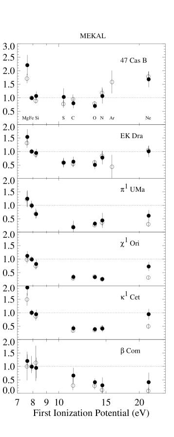
The abundances found with the different methods are listed in Table 9 and plotted as a function of the FIP in Figure 8. We plot the abundance ratios $A$/Fe with respect to the solar photospheric ratios as a function of the FIP. The open circles represent the coronal abundances derived from method 1 whereas the filled circles show the abundances derived from method 2. We find a good agreement between the abundance sets, and an acceptable overall agreement between the results using the MEKAL database and the APEC database.

Nevertheless, some differences can be noted in Table 9. In the older stars $\chi^{1}$ Ori, $\kappa^{1}$ Cet, and $\beta$ Com, some systematic differences occur for the C/Fe abundance ratios, the abundances derived with APEC being smaller than those derived with SPEX although the error ranges are large. For the same stars, some differences are also present in the N/Fe abundance ratio. In both cases, the abundances are determined from only one faint line (C vi and N vii, respectively), making the measurements of the line fluxes difficult (see Tables 5 and 6). Differences also occur in the four older stars for the Ne/Fe abundance ratio. This is partly due to the lack of strong and reliable (i.e., unblended) Ne lines. While in hot coronae, the strong Ne x line serves as a reliable indicator for the Ne abundance, this line is much weaker in cooler coronae and strongly blended with Fe lines. The Ne ix lines at 13.55–13.7 Å are always blended with Fe lines, but also become quite faint in the less active stars. Further, the inferred Ne flux in the line feature depends on the absolute Fe abundance. The latter is poorly determined in particular in the less active stars where almost no continuum is present. We emphasize that we cannot attribute the discrepancy to any of the methods. The available data quality simply makes the determination of the Ne/Fe abundance ratio in cooler coronae ambiguous.

Fe blending leads to some differences in the Mg/Fe abundances as well (the largest deviations are for $\pi^{1}$ UMa using APEC method 2, and $\kappa^{1}$ Cet using SPEX method 2). Finally the weakness of the S lines in the more active stars leads to some differences in the S/Fe abundances.

The absolute Fe abundance was systematically higher when the APEC database was used. Note that in the spectrum of $\beta$ Com, the continuum is almost nonexistent and the derivation of the Fe abundance is difficult. For the latter target, the $\delta$-fit did not converge for the Ne line with APEC. For this reason, these two points are missing in Table 9 and Figure 8.

However, we recognize many of these features to be due to limitations of the data and the reconstruction methods. On the other hand, these systematic differences are small compared to the general trends. As shown in Figure 8, the abundances resulting from the two methods and the two databases agree mostly quite well within the errors, and the general trends are the same, regardless of the method used.

6.3. Light curves

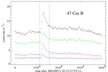
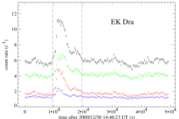
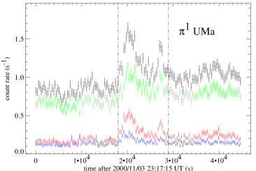
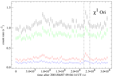
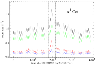
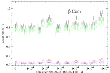
The light curves of the six stars are shown in Figure 9. For each star, four light curves are plotted. They describe, from top to bottom, the total count rates in the $0.2-10$ keV range (black), in the soft band ($0.2-1$ keV, green), in the hard band ($>1$ keV, third plot), and the ratio between the hard and the soft count rates (blue). The upper energy thresholds used for the hard band vary from star to star and are listed in Table 4. Only data from detectors that operated in imaging mode were considered (for 47 Cas B, EK Dra and $\beta$ Com, the data from MOS1, MOS2 and PN were used; for $\pi^{1}$ UMa, data from MOS1 and MOS2, and for $\chi^{1}$ Ori and $\kappa^{1}$ Cet, only data from one MOS camera, MOS2 and MOS1 respectively, were used).

The light curves display considerable variability. We observe the presence of large flares on all stars in our sample except $\beta$ Com. However, even after excluding these flares, the light curves still show considerable variability that cannot be described by steady, quiescent coronal emission. We also note that the hard emission becomes weaker toward older stars, in agreement with the decline of the average coronal temperature described earlier.

7. Discussion

7.1. Correlation between the Parameters

The results of our analysis of six solar analogs clearly show a number of trends that we wish to quantify below using our results from method 2. Before doing so, we note that the X-ray results from the observation of $\kappa^{1}$ Cet are rather similar to results from $\pi^{1}$ UMa and $\chi^{1}$ Ori, despite the former’s significantly longer rotation period and, hence, higher age. The reason for this discrepancy is not entirely clear, but we note that $\kappa^{1}$ Cet has a slightly later spectral type and therefore a somewhat lower mass than the other targets. It is known that later-type stars evolve more slowly (Soderblom et al., 1993) and that they remain in a state of maximum X-ray luminosity (the saturation limit) for longer rotation periods (Pizzolato et al., 2003) than stars of earlier spectral type. Both effects make $\kappa^{1}$ Cet look somewhat younger than inferred from a rotation-activity relation that is appropriate for early G stars.

In Figure 10, we plot the mean coronal temperature, $\bar{T}$, (see Table 7) as a function of the total luminosity $L_{\mathrm{X}}$. We fitted the data with a power-law. Because both variables to be correlated are likely to be affected by systematic scatter around any power-law, we use the ordinary least squares bisector method as described by Isobe et al. (1990). Clearly, the two parameters are correlated. We find, for our results from MEKAL and APEC, respectively,

$$L_{X} \approx 1.17\times 10^{26}\bar{T}^{4.26\pm 0.41}\rm\qquad erg\,s^{-1}~{}(MEKAL),$$ (6)

$$L_{X} \approx 1.61\times 10^{26}\bar{T}^{4.05\pm 0.25}\rm\qquad erg\,s^{-1}~{}(APEC),$$ (7)

where $\bar{T}$ is in MK. These relations are consistent with the results of Güdel et al. (1997a), except that the latter authors used the higher temperature for a model with two thermal components fitted to ROSAT spectra. Two points for the Sun at minimum and maximum activity level are also plotted for comparison (after Peres et al. 2000).

In Figure 11 the temperature as a function of the period is shown. Again, we fitted the data with a power-law. In this case, the relations calculated from the two power-laws are given by

$$\bar{T} \approx 11.6P_{\rm rot}^{-0.48\pm 0.07}\rm\qquad MK~{}(MEKAL),$$ (8)

$$\bar{T} \approx 12.2P_{\rm rot}^{-0.50\pm 0.08}\rm\qquad MK~{}(APEC),$$ (9)

where $P_{\rm rot}$ is the rotation period in days. Similar results were obtained for the ROSAT data by Güdel et al. (1997a), again considering the higher fit-temperature instead of the mean temperature. As we averaged the temperature with the EM in each bin used as weights, the steady decrease of the mean temperature with period is consistent with a decrease of the amount of hot plasma as the star spins down.

Equations 6–9 allow us to check for consistency with published relations between $L_{\rm X}$ and $P_{\rm rot}$. By combining formula (6) with (8) or, respectively, (7) with (9), we find

$$L_{\rm X} = 4.01\times 10^{30}P_{\rm rot}^{-2.04\pm 0.36}\rm\quad erg~{}s^{-1}~{}(MEKAL),$$ (10)

$$L_{\rm X} = 4.04\times 10^{30}P_{\rm rot}^{-2.03\pm 0.35}\rm\quad erg~{}s^{-1}~{}(APEC),$$ (11)

which is consistent with previously reported dependences of this type (Pallavicini et al., 1981; Güdel et al., 1997a). A linear regression for $\log L_{\rm X}$ and $\log P_{\rm rot}$ yields the same result, with a power-law index of –2.03.

We also studied the relation between radio luminosity and the temperature. Radio luminosities or upper limits thereof are available (Güdel & Gaidos, 2001) for five out of the six targets and are plotted in Figure 12. They refer to low emission levels outside obvious flares. We use the values of the upper limits in the regression analysis. The slopes of the power-laws are therefore lower limits, given by

$$L_{R} \approx 0.86\times 10^{9}\bar{T}^{5.65\pm 0.46}\rm\qquad erg\,s^{-1}\,Hz^{-1}~{}(MEKAL),$$ (12)

$$L_{R} \approx 1.69\times 10^{9}\bar{T}^{5.29\pm 0.74}\rm\qquad erg\,s^{-1}\,Hz^{-1}~{}(APEC).$$ (13)

These relations suggest a relation between the nonthermal electron population, responsible for radio gyrosynchrotron emission, and coronal heating.

7.2. Abundances

In the solar corona, the so-called FIP effect has been observed, in which the elements with a FIP lower than 10 eV are overabundant relative to the solar photospheric composition, whereas the elements with a higher FIP show the same abundance as the solar photosphere (Feldman, 1992; Laming et al., 1995; Feldman & Laming, 2000). Recent spectroscopic analysis with XMM-Newton and Chandra has shown that in very active stars, an inverse effect is present, in which the low-FIP elements are depleted relative to the high-FIP elements (Brinkman et al., 2001). In our sample, we observe an evolutionary trend from an inverse FIP effect for the most active star 47 Cas B to a solar-like FIP effect in the oldest stars (Figure 8). We note, however, that the absolute abundances of low-FIP elements such as Fe do not reach values as high as in the solar corona, where overabundances by factors of a few are common (Feldman, 1992).

In Figure 13, the abundances of Fe, Ne, and the ratios $A$(Ne)/$A$(Fe), $A$(O)/$A$(Ne), $A$(O)/$A$(Fe), and $A$(Mg)/$A$(Fe) are plotted as a function of the temperature (based on MEKAL/SPEX, method 2). The dotted regions include the ranges of a larger stellar sample (Güdel, 2004). The abundance of the low-FIP element Fe tends to decrease from a nearly photospheric value for stars with an average temperature of 3 to 5 MK to a lower abundance of $\approx$ 0.5 for the two more active stars EK Dra and 47 Cas B. The error bars for the coolest star ($\beta$ Com) are not plotted for Fe and Ne, since they exceed the range illustrated in the figures. This is due to the near-absence of a continuum in this star, which makes absolute abundance determinations difficult. The abundance ratios, however, are robust (see also Audard et al. 2004).

In the middle left and the bottom left panels, the abundance ratio of Ne/Fe and O/Fe, respectively, are shown as a function of the average coronal temperature. Because Ne and O are high-FIP elements, and Fe is a low-FIP element, the ratios increase with temperature, confirming the evolutionary trend of decreasing low-FIP elements (such as Fe) with increasing activity. A similar effect was found by Audard et al. (2003a) for a sample of active RS CVn-type binaries. This is also confirmed by a larger sample of active stars (Güdel, 2004).

The plots in the middle right and bottom right panels show the abundance ratio of O/Ne, two high-FIP elements, and of Mg/Fe, two low-FIP elements. Our sample of stars is too small to constrain a trend in these plots. However, the larger star sample studied by Güdel (2004) shows a nearly flat distribution for both ratios.

Could it be that the coronal abundance pattern reflects the composition of the underlying photosphere? This view does not find support from other studies. Although a full picture would include knowledge of the abundances of other elements such as C, N, O, we see, from the summary in Sect. 2.2, no support for a photospheric abundance pattern that significantly deviates from solar. Finally, we recall that the solar coronal composition does not reflect the photospheric composition either, hence an agreement between photospheric and coronal abundances is not a priori anticipated for solar analogs.

7.3. Flares and Coronal Heating

In the previous sections, we have highlighted correlations between observable parameters, and we have found continuous variability in all six targets to an extent that hardly any time interval is free of fluctuations. Although conventional interpretation of coronal structure often makes use of the approximation of static coronal loops (as, e.g., described by Rosner et al. 1978), the interpretation of the phenomenology revealed by our light curves cannot be rooted in strictly static loops, although static loop models may, under certain circumstances, serve as approximations even under flaring conditions (Jakimiec et al., 1992).

There is appeal in the alternative, extreme model assuming that the coronal emission is entirely due to dynamic, flaring loops. A number of observed features reported in this paper and in the previous literature seem to support such a model: i) with the sensitivity available with XMM-Newton and Chandra, X-ray emission previously ascribed to a quiescent component is now recognized to be continuously variable; in the most extreme cases, no steady component can reasonably be identified in the light curves (Audard et al., 2003b). ii) More active stars (i.e., stars with a higher $L_{\rm X}/L_{\rm bol}$ ratio) appear to maintain hotter coronae. This is difficult to explain with a model that assumes a corona composed only of steady magnetic loops, with the principal determinant of $L_{\rm X}$ being the magnetic filling factor, up to the empirical saturation value of $\log L_{\rm X}/L_{\rm bol}\approx-3$. Such models do not automatically explain why the coronal temperature increases with increasing $L_{\rm X}$. We discuss this point further in our conclusions below. iii) Active stars continuously produce radio emission from accelerated electrons. The lifetime of the latter is short, probably amounting to no more than seconds to minutes (Kundu et al., 1987). In the solar corona, flare energy-release processes are required to produce such electron populations. In order to generate the observed stellar radio emission, high-energy electrons must be replenished frequently.

This question has previously been addressed by studying, for a model in which the corona is heated entirely by flares, the EMD (Güdel, 1997c; Güdel et al., 2003), the average temperature to be ascribed to such a corona (Audard et al., 2000), and the light curve characteristics expected from a superposition of stochastic flares (Audard et al., 1999, 2000; Kashyap et al., 2002; Güdel et al., 2003; Arzner & Güdel, 2004). We are now in a position to apply the methodology to our results.

First, we use the shapes of our EMDs to characterize the underlying flare population in the framework of this model. Güdel et al. (2003) derived an analytic expression for a DEM of a flare-heated corona under the assumption that the temperature and the flare density both decay exponentially with time constants $\tau_{T}$ and $\tau_{n}$, respectively, and that a relation between flare peak-EM and peak-$T$ holds, EM${}_{p}\propto T_{p}^{b}$, as reported by Feldman et al. (1995). Then, the DEM follows power-law relations on both sides of its peak temperature ($T_{m}$), with

$$Q(T)\propto\left\{\begin{array}[]{ll}T^{2/\zeta}&,T\leq T_{m}\\ T^{-(b-\phi)(\alpha-2\beta)/(1-\beta)+2b-\phi}&,T\geq T_{m}\end{array}\right.$$ (14)

where $b\approx 4.3\pm 0.35$ as derived from a large sample of stellar flares (Güdel, 2004). The temperature $T_{m}$ depends on the energy of the smallest flares participating in the heating in this simple model (Güdel et al., 2003). Further, $\beta$ is a power-law index for a relation between the flare e-folding decay time and its radiated energy, $\tau\propto E^{\beta}$. As noted by Güdel et al. (2003), $\beta$ is probably close to zero although an extreme case of $\beta=0.25$ was also studied. The variable $\phi$ gives the slope of the cooling function (radiative power per unit emission measure) for a power-law approximation in the temperature interval of interest. We use $\phi=-0.3$ as an approximation of the slope of the cooling function in the logarithmic temperature interval 6.8–7.5, i.e. the temperature interval above the EMD peak temperature (see Fig. 10 in Audard et al. 2004). The parameter $\alpha$ is of primary interest for us: It is the exponent of the distribution of the occurrence rate $N$ of flares in radiated energy, viz., $dN/dE\propto E^{-\alpha}$ as found for a large sample of solar flares (e.g., Crosby et al. 1993), but applicable also to stellar coronae (see references above). In the first equation, applicable to the cooler portion of the DEM, $\zeta=\tau_{n}/\tau_{T}$. This parameter describes the amount of heating occurring during the flare decay, with $\zeta=2$ corresponding to free cooling without heating, and $\zeta\approx 0.5$ corresponding to extreme heating rates during the decay (Reale et al., 1997).

We have measured the slopes of our EMDs on both sides of $T_{m}$. To find the possible ranges for the best-fit slopes, we re-analyzed our data using method 2 by starting with different initial conditions for the slopes in our iteration, but the DEMs converged to similar values. The ranges of the resulting best fit slopes (not considering the error ranges in the DEM) are reported in Table 10. We then used Eq. 14 to determine the most likely $\zeta$ and $\alpha$ with their acceptable ranges. The results are also reported in Table 10.

From the low-$T$ slopes of the EMDs derived with method 2 using SPEX, we find $\zeta$ to be around unity in all cases. Such values are typical for individual flares observed on active stars (see Güdel et al. 2003 and references therein) and support our assumption that such flares contribute significantly to the overall observed emission. Static loops, on the other hand, normally produce shallower DEMs, with slopes of +1 to +3/2, depending on the amount of conductive flux at the loop footpoints (Rosner et al., 1978; van den Oord et al., 1997).

From the high-$T$ slope, we derive $\alpha\approx 2.2-2.8$, in excellent agreement with $\alpha$ values determined from long light curves of active stars (Audard et al., 2000; Kashyap et al., 2002; Güdel et al., 2003; Arzner & Güdel, 2004). If $\alpha>2$ and the emitted energy is integrated over the flare-rate distribution to obtain the total radiative loss, i.e., $L_{\rm tot}=\int_{E_{1}}^{E_{2}}E(dN/dE)dE$, then $L_{\rm tot}$ diverges as $E_{1}\rightarrow 0$, i.e., the smallest flares dominate coronal heating, and a lower energy cutoff is required for this power-law.

We now continue this consideration by simulating light curves based on a characteristic flare shape for the three most active stars, assuming a flare-rate distribution based on $\alpha$ as determined above. The flare shape was derived from the convolution of an exponential function (cut off at t $<$ 0, describing the decay) and a Gaussian (important to describe the rise and the peak phase). The shapes of the largest flares in the light curves were used to estimate the characteristic rise and the decay time parameters. We performed two sets of simulations: one with $\beta$ = 0 and one with $\beta$ = 0.25. In each simulation $\alpha$ was chosen within the acceptable range for a given $\beta$. The flare decay-time was varied according to the scaling $\tau\propto E^{\beta}$. For the largest flare in each light curve, we measured the amplitude and fitted the decay phase with an exponential function to find the decay time, and hence the emitted energy. We then set the maximum flare energy $E_{2}$ equal to the energy of the largest observed flare and constructed a power-law distribution of flares in energy, down to a selectable minimum flare energy $E_{1}$. The flares were randomly distributed in time (assuming a total of 40 ks), and their light curves were superimposed. The rate of flares at a given energy, equivalent to the probability of the largest flares to occur within the simulation time, could be statistically varied. We measured the modulation depth, i.e., the ratio between the root-mean-square scatter of the light curve and the average luminosity, and compared it with the same measure for the observed light curves outside the outstanding largest one or two flares. The minimum flare energy $E_{1}$ and the numbers of large flares occurring was varied until the modulation depth and the average luminosity level agreed with the observed light curves. The modulation depth of the observed light curves is given in Table 10. It increases with decreasing activity. The simulated light curves, for $\beta$ = 0 and $\alpha$ = 2.25, 2.28, and 2.54 for 47 Cas, EK Dra, and $\pi^{1}$ UMa respectively, are shown in Figure 14. The range $\log E_{2}/E_{1}$ (in dex) of flare energies thus required for the light curve is also given in Table 10.

We see that typically 1.8$-$5.3 orders of magnitude of flare energies for $\beta$ = 0 and 1.8$-$6.8 for $\beta$ = 0.25, respectively, are required to “describe” our light curves. The interesting point is that this range is larger for the more luminous stars. This can be understood because a narrow range of flare energies produces a more strongly modulated light curve, while a large number of small flares merely adds a quasi-steady baseline level. However, in Equation 14, the turnover in the DEM is determined by the smallest flares participating in the statistics. One would thus expect that $E_{1}$ decreases with decreasing activity, contrary to the results in Table 10. However, we emphasize that our light curve model is based on the extreme assumption that all emission originates from flares. If there is a steady baseline level of X-ray emission not directly related to flare decays, as suggested from solar observations, we can obviously not determine $E_{1}$ from light curve analysis. Also, our model does not take into account any possible change in $\alpha$ at lower energies. We know from solar observations that there will be a continuation toward smaller flares as well, rather than a lower energy threshold. The values in Table 10 are therefore only indicative of the range of flare energies required in the most extreme model discussed here.

8. Conclusions

As the rotation rate of a solar analog decreases during its evolution on the main sequence, the efficiency of the internal dynamo weakens, resulting in a decrease of the magnetic activity in the stellar atmosphere. We have studied systematic trends in the long-term evolution of stellar coronal X-ray emission for ages in the range 0.1–2 Gyr. As a consequence of the stellar spin-down, the X-ray luminosity steadily decreases from levels that may be close to the empirical saturation limit in the youngest stars ($L_{X}/L_{\rm bol}\approx 10^{-3}$), to levels approximately two orders of magnitude lower within the first two Gyr. During the next $\approx$3–4 Gyr, $L_{X}$ reduces by another factor of ten to levels as seen in $\alpha$ Cen, $\beta$ Hyi, or the Sun (Güdel et al., 1997a). The overall trends reported here confirm earlier studies based on lower-resolution X-ray spectroscopy (Maggio et al., 1987; Güdel et al., 1997a).

The high-resolution X-ray spectroscopy now available has permitted a more detailed study of the composition and the thermal structure of solar-like coronae than was previously possible. We have studied emission measure distributions and coronal element abundances for all six targets in a homogeneous way, applying two widely differing methods and using two different sets of atomic parameters. It is important to recall that both of our methods include modeling of line blends to the extent possible with the presently available line emissivities.

There is gratifying agreement between the results from the two methods, although it appears that the choice of the atomic database introduces systematic differences. This is perhaps not surprising as the presently available compilations of atomic parameters are incomplete and suffer from systematic uncertainties. A more serious limitation is set by the mathematical problem of spectral inversion itself. While even counting statistics at the percent level makes the inversion problem ill-conditioned (Craig & Brown, 1976; Judge, 2002), systematic uncertainties in the line emissivities of perhaps up to 10–20% may introduce various structure in our EMDs that may not correspond to coronal features. We have suggested that a reasonable convergence criterion should be set, although it is difficult to assess at what level artificial structure is introduced into a reconstructed EMD. Regardless of these inconsistencies, however, we recover element abundances that are rather robust.

With these limitations in mind, we have found systematic trends in the EMD structure as a star ages. Not only does the total emission measure continuously decrease, the temperature where the EMD peaks also decays with time. The EM-weighted logarithmic average of the coronal temperature $\bar{T}$ thus follows a power-law dependence on the X-ray luminosity, namely $\bar{T}\propto L_{X}^{0.25\pm 0.02}$. A similar relation between the dominant coronal temperature and $L_{\rm X}$ was already studied by Schrijver et al. (1984), using Einstein data of a large sample of stars. Schmitt et al. (1990) found for 1-$T$ model fits $T\propto L_{X}^{0.4}$ from Einstein data. Finally, Güdel et al. (1997a) used ROSAT data and a G-star sample similar to ours and found a relation between the higher temperature of a 2-$T$ model and $L_{\rm X}$ in complete agreement with our results.

The observed trends cannot be explained by a model that is based exclusively on different filling factors of the surface magnetic field, as an increased filling factor does not explain per se why the temperature should increase. We have discussed an extreme case of an alternative model in which a statistical distribution of flares is responsible for the correlation between $L_{\rm X}$ and $\bar{T}$. The question then is why the flare rate (above any given base-level energy) is higher in more active (i.e., more rapidly rotating) stars. Our data cannot give a conclusive answer. One possibility is that more active stars indeed do show a larger magnetic surface filling factor, and that the higher density of magnetic loops leads to more magnetic reconnection, thus producing a higher flare rate (Güdel et al., 1997a); this, then, also includes a more prominent population of very large flares that produce both large emission measures and very high temperatures, thus shifting the average temperature to higher values. Once the magnetic filling dilutes, the interactions between neighboring magnetic loop systems will become less frequent, and both $L_{\rm X}$ and $\bar{T}$ decrease (see Güdel et al. 1997a).

Alternatively, instead of increasing the surface filling factor, other ingredients may systematically change with changing rotation period, such as the structure of surface magnetic field in active regions or differences in the convection pattern that jostles the magnetic-loop footpoints. In a statistical-flare model, then, the way to explain the $L_{\rm X}-\bar{T}$ correlation would be to reheat the same active regions more frequently in more active stars, as some process brings non-potential energy into the magnetic fields at a higher rate. As argued by Audard et al. (2000), such frequently-heated loops can be approximated by static loops although the heating process is non-static. In this case, approximating the loop temperature with its apex temperature (where most of the EM is found), the Rosner et al. (1978) loop scaling law predicts $L_{\rm X}\propto T^{3.7}$ for loops of given length below the coronal pressure scale height, and $L_{\rm X}\propto T^{4.7}$ for loops larger than this limit (see Audard et al. 2000 for details). These predictions are close to our observational finding. On the other hand, static loops would predict slopes of the DEM on the low-temperature side that are significantly smaller than those determined by us.

To conclude, we are presently unable to distinguish between a model in which the flare rate is controlled by the magnetic filling factor, and one in which constrained active regions flare progressively more frequently as the rotation rate of a star increases. Both approaches, however, are compatible with the hypothesis that much of the coronal heating is induced by flaring, regardless of the ultimate cause of the increased flare rate in more active stars.

Because larger flares produce hotter plasma (Feldman et al., 1995), more active stars produce hotter coronae. This trend is unequivocally recovered from our observations and further supports a picture in which flares contribute significantly to the overall coronal heating (e.g., Audard et al. 2000; Kashyap et al. 2002; Güdel et al. 2003).

We note in passing that an alternative view with similar consequences has recently been presented by Peres et al. (2004). These authors suggest that, based on properties of coronal structures seen on the Sun, a higher occurrence of very compact, hot features including flares make more active coronae hotter.

We have also derived element abundances and found good agreement between our two methods. Somewhat more systematic deviations can be noted if different atomic databases are used (MEKAL, APEC), but the trends in the abundance pattern agree and markedly change with changing activity level. A similar trend was noted for RS CVn binaries by Audard et al. (2003a), but the latter study referred to extremely active stars in which the abundance pattern changed from a strong inverse FIP effect to a flat distribution with decreasing activity (or mean coronal temperature). In our sample, the change from an inverse or flat distribution to a solar-like distribution occurs at ages of less than 300 Myr or rotation periods longer than $\approx$ 3 days. Incidentally, a rapid decay of nonthermal radio emission has been noted for the same activity range. We hypothesize that the same electrons that are responsible for the observed gyrosynchrotron emission also induce an inverse-FIP effect in the most active stars, as follows (see Güdel et al. 2002 for further arguments): if electrons are streaming along the magnetic fields toward the chromosphere, they build up a downward-pointing electric field that acts to suppress positive currents from the chromosphere to the corona. In other words, ions in the chromosphere are prevented from streaming into the corona, while neutral, predominantly high-FIP elements, are not affected. As the electron population diminishes in less active stars, the suppression of ion diffusion into the corona disappears, and a solar-like FIP effect can build up, by whatever (still unidentified) mechanisms. Recently, Laming (2004) presented an alternative model in which both the solar-like FIP and the inverse FIP effect are related to a common plasma-physical cause.

Note added in proof. $-$ In a recent publication, Antia & Basu (2005, ApJ, 620, L129) suggested that a significant discrepancy between helioseismological studies and modeling of the solar interior, brought about by new measurements of a lower solar photospheric abundance of oxygen, may be resolved by an upward revision of the solar photospheric neon abundance. They therefore predict a solar photospheric O/Ne abundance ratio lower than that adopted here. This may explain the generally low value of the coronal O/Ne abundance ratio observed in the coronae of stars, including our sample stars (Fig. 13), regardless of activity level (see also Fig. 37 in Güdel 2004).

Table 1Program stars, including a comparison with the Sun

Star	Spec.	Distance	$P_{\rm rot}$	$\log L_{X}$	$\log L_{X}$	$\log L_{X}$	Age
	type	(pc)	(d)	(erg s-1)	(erg s-1)	(erg s-1)	(Gyr)
47 Cas B	G0-2 V	33.56	$\approx$1.0	30.31	30.35	30.39	0.1
EK Dra	G0 V	33.94	2.75	29.93	30.06	30.08	0.1
$\pi^{1}$ UMa	G1 V	14.27	4.7	29.10	29.05	29.06	0.3
$\chi^{1}$ Ori	G1 V	8.66	5.1	28.99	28.95	28.95	0.3
$\kappa^{1}$ Cet	G5 V	9.16	9.2	28.79	28.94	28.95	0.75
$\beta$ Com	G0 V	9.15	12.4	28.21	28.26	28.26	1.6
Sun	G2 V	$5\times 10^{-6}$	25.4	27.3	27.3	27.3	4.6

Table 2Stellar photospheric abundances

Star	Fe	Mg	Si	S	C	O	N	Ref.
EK Dra	$1.20$	$-$	$-$	$-$	$-$	$-$	$-$	1
$\pi^{1}$ UMa	0.83-1.02	0.65-0.83	0.78-1.12	$-$	$-$	$-$	$-$	2
	0.93 (0.81-1.07)	0.74 (0.58-0.95)	0.89 (0.83-0.95)	$-$	0.85 (0.68-1.07)	$-$	$-$	3
	$0.87$	$-$	$-$	$-$	$-$	$-$	$-$	1
	$1.10$	$-$	$-$	$-$	$-$	$-$	$-$	4
	0.83-0.98	$-$	$-$	$-$	$-$	$-$	$-$	5
	1.09 (1.00-1.19)	$-$	$-$	$-$	$-$	$-$	$-$	6
$\chi^{1}$ Ori	0.89-0.93	$0.91$	$0.98$	$-$	$-$	$-$	$-$	7
	$0.91$	$-$	$-$	$-$	$-$	$-$	$-$	8
	$\approx 1$	$-$	$-$	$-$	$0.63$	$-$	$-$	9
	1.14 (1.07-1.22)	$-$	$-$	$-$	$-$	$-$	$-$	6
	$1.35$	$-$	$-$	$-$	$-$	$-$	$-$	1
	0.66-1.29	$-$	$-$	$-$	$-$	$-$	$-$	5
$\kappa^{1}$ Cet	0.89-1.04	0.85-0.98	0.95-1.07	$-$	$-$	$-$	$-$	2
	1.29 (1.17-1.41)	0.91 (0.76-1.10)	0.85 (0.78-0.93)	$-$	0.91 (0.71-1.17)	$-$	$-$	3
	$1.0$	$-$	$-$	$-$	$-$	$-$	$-$	7
	$1.13$	$-$	$-$	$-$	$-$	$-$	$-$	6
	$1.66$	$-$	$-$	$-$	$-$	$-$	$-$	1
	0.98-1.10	$-$	$-$	$-$	$-$	$-$	$-$	5
$\beta$ Com	$0.93$	$-$	$-$	$1.38$	$0.98$	1.26 (1.05-1.47)	$1.05$	10
	1.00-1.07	$1.17$	$1.00$	$-$	$-$	$-$	$-$	7
	1.15 (1.07-1.25)	$-$	$-$	$-$	$-$	$-$	$-$	6
	$1.07$	$-$	$-$	$-$	$-$	$-$	$-$	1
	$1.00$	$-$	$-$	$-$	$-$	$-$	$-$	8
	$1.17$	$-$	$-$	$-$	$-$	$-$	$-$	4
	0.89-1.17	$-$	$-$	$-$	$-$	$-$	$-$	5

Note. — Values refer to the solar photospheric composition. If available, error ranges are given in parentheses.

References. — (1)Rocha-Pinto et al. (2004); (2) Ottmann et al. (1998); the original values were transformed to solar abundances as given by Anders & Grevesse 1989 = AG89 except for Fe for which we use the value given in Grevesse & Sauval 1999 = GS99; (3) Gaidos & Gonzalez (2002); (4) Gray et al. (2001) ; (5) Cayrel de Strobel et al. (2001); (6) Taylor (2003), corrected to GS99; (7) Edvardsson et al. (1993); (8) Gratton et al. (1996); (9) Tomkin et al. (1995), corrected to AG89 and GS99; (10) Clegg et al. (1981).

Table 3Observation log

Star	Instruments	Filter	Start	Stop	Exposure [s]
47 Cas B	RGS 1	-	2001/09/10 23:30:24	2001/09/11 13:39:00	36610
	RGS 2	-	2001/09/10 23:30:24	2001/09/11 13:39:01	36610
	MOS 1	Thick	2001/09/11 02:04:32	2001/09/11 13:29:30	36610
EK Dra	RGS 1	-	2000/12/30 14:01:58	2000/12/31 05:17:04	41960
	RGS 2	-	2000/12/30 14:01:58	2000/12/31 05:17:04	41960
	MOS 2	Thick	2000/12/30 14:10:36	2000/12/31 04:38:02	41960
$\pi^{1}$ UMa	RGS 1	-	2000/11/03 21:44:48	2000/11/03 12:28:18	38800
	RGS 2	-	2000/11/03 21:44:48	2000/11/03 12:28:19	38800
	MOS 1	Thick	2000/11/03 21:53:16	2000/11/03 11:49:04	38800
$\chi^{1}$ Ori	RGS 1	-	2001/04/07 08:56:49	2001/04/07 22:31:53	29326
	RGS 2	-	2001/04/07 08:56:49	2001/04/07 22:31:59	29326
	MOS 2	Thick	2001/04/07 09:03:11	2001/04/07 17:45:10	29326
$\kappa^{1}$ Cet	RGS 1	-	2002/02/09 16:13:01	2002/02/10 03:21:41	35920
	RGS 2	-	2002/02/09 16:13:01	2002/02/10 03:21:35	35920
	MOS 1	Thick	2002/02/09 16:19:33	2002/02/10 03:18:09	35920
$\beta$ Com	RGS 1	-	2003/07/20 02:08:16	2003/07/20 20:13:28	61320
	RGS 2	-	2003/07/20 02:08:16	2003/07/20 20:13:34	61320
	MOS 2	Thick	2003/07/20 02:09:06	2003/07/20 19:12:36	61320

Table 4Spectral wavelength ranges used for method 1

Instrument	$\lambda$ range (Å)
RGS	$8.30-9.50$
RGS	$12.00-13.95$
RGS	$14.15-15.90$
RGS	$16.20-17.15$
RGS	$17.80-18.30$
RGS	$18.75-19.20$
RGS	$20.80-21.10$
RGS	$21.40-22.40$
RGS	$23.65-24.00$
RGS	$24.50-24.90$
RGS	$28.50-30.10$
RGS	$31.10-32.00$
RGS	$33.40-33.85$
MOS	$1.70\tablenotemark{a}-6.90$
MOS	$7.80-9.35$

Table 5Lines used for the EMD reconstruction. Method 2, with MEKAL/SPEX

Line	$\log T_{m}$  (K)	$\lambda$ (Å)	47 Cas B	EK Dra	$\pi^{1}$    UMa	$\chi^{1}$ Ori	$\kappa^{1}$ Cet	$\beta$ Com
Fe xvii	6.7	15.01	483.2$\pm$17.2	376.9$\pm$13.9	61.5$\pm$2.4	52.0$\pm$1.6	43.5$\pm$1.4	8.5$\pm$0.5
Fe xvii	6.7	16.78	217.5$\pm$12.3	152.7$\pm$9.4	29.3$\pm$1.8	24.1$\pm$1.1	24.8$\pm$1.1	4.3$\pm$0.4
Fe xviii	6.8	14.20	292.9$\pm$15.2	207.4$\pm$11.7	20.5$\pm$1.6	17.0$\pm$1.0	16.2$\pm$1.0	1.4$\pm$0.3
Fe xix	6.9	13.52	222.9$\pm$26.6	126.6$\pm$19.6	14.5$\pm$2.9	8.3$\pm$1.6	6.8$\pm$1.5	0.8$\pm$0.6
Fe xx	7.0	12.83	289.7$\pm$21.9	162.5$\pm$59.0	7.4$\pm$1.8	4.3$\pm$1.1	5.8$\pm$1.0	$-$
Fe xxi	7.0	12.29	210.2$\pm$24.7	149.1$\pm$16.3	8.3$\pm$2.1	7.3$\pm$1.3	8.7$\pm$1.4	$-$
Fe xxiii	7.2	11.74	183.3$\pm$21.5	116.5$\pm$15.1	$-$	$-$	$-$	$-$
Fe xxiv	7.3	10.62	95.0$\pm$40.1	55.8$\pm$13.1	$-$	$-$	$-$	$-$
Fe xxv	7.8	1.85	68.0$\pm$17.8	22.6$\pm$81.0	$-$	$-$	$-$	$-$
O viii	6.5	18.97	639.8$\pm$17.6	298.5$\pm$11.5	32.2$\pm$1.7	28.2$\pm$1.1	29.5$\pm$1.1	5.6$\pm$0.4
O vii	6.3	21.60	90.2$\pm$11.8	50.1$\pm$8.2	11.6$\pm$1.6	8.6$\pm$1.0	10.1$\pm$0.96	2.4$\pm$0.5
O vii	6.3	22.10	48.6$\pm$10.2	39.5$\pm$7.7	8.4$\pm$1.5	6.5$\pm$0.8	6.1$\pm$0.9	3.3$\pm$0.5
C vi	6.1	33.73	68.2$\pm$7.9	38.1$\pm$5.2	2.6$\pm$2.3	3.6$\pm$0.5	4.1$\pm$0.6	1.3$\pm$0.3
N vii	6.3	24.77	62.2$\pm$8.9	32.3$\pm$5.1	3.8$\pm$1.5	1.8$\pm$0.4	2.5$\pm$0.4	0.4$\pm$0.3
Ne x	6.8	12.13	475.0$\pm$33.3	185.7$\pm$21.2	$-$	$-$	$-$	$-$
Ne ix	6.6	13.45	277.8$\pm$27.6	113.0$\pm$17.9	8.4$\pm$2.3	8.9$\pm$1.5	10.0$\pm$1.5	0.9$\pm$0.5
Ne ix	6.6	13.70	$-$	$-$	5.9$\pm$2.0	5.2$\pm$1.2	6.4$\pm$1.2	$-$
Mg xii	7.0	8.42	238.7$\pm$13.2	93.9$\pm$8.1	3.9$\pm$0.7	2.5$\pm$0.4	6.1$\pm$0.5	0.3$\pm$0.2
Mg xi	6.8	9.17	320.6$\pm$10.8	157.2$\pm$7.1	15.0$\pm$0.7	10.4$\pm$0.4	14.7$\pm$0.5	1.5$\pm$0.1
Si xiv	7.2	6.18	114.2$\pm$12.0	57.3$\pm$7.9	$-$	$-$	$-$	$-$
Si xiii	7.0	6.65	194.0$\pm$11.0	105.6$\pm$7.5	5.6$\pm$0.6	4.9$\pm$0.4	5.7$\pm$0.4	0.7$\pm$0.2
S xvi	7.2	4.72	55.6$\pm$12.0	$-$	$-$	$-$	$-$	$-$
S xv	7.2	5.04	93.3$\pm$11.3	35.7$\pm$6.3	$-$	$-$	$-$	$-$

Table 6Lines used for the EMD reconstruction. Method 2, with APEC/XSPEC

Line	$\log T_{m}$  (K)	$\lambda$ (Å)	47 Cas B	EK Dra	$\pi^{1}$ UMa	$\chi^{1}$ Ori	$\kappa^{1}$ Cet	$\beta$ Com
Fe vii	6.7	15.01	477.5$\pm$19.6	378.7$\pm$16.3	61.5$\pm$2.9	51.9$\pm$1.7	44.2$\pm$1.8	8.1$\pm$ 0.7
Fe vii	6.7	16.78	222.3$\pm$18.6	150.5$\pm$15.2	30.9$\pm$2.7	25.1$\pm$1.8	25.5$\pm$1.6	4.5 $\pm$0.7
Fe viii	6.9	14.20	297.4$\pm$18.9	207.1$\pm$15.9	20.4$\pm$2.7	17.2$\pm$1.3	16.9$\pm$1.3	1.4 $\pm$0.6
Fe xix	6.9	13.52	235.2$\pm$39.8	114.7$\pm$34.0	14.4$\pm$2.3	5.8 $\pm$2.8	6.6$\pm$2.2	0.7$\pm$0.6
Fe xx	7.0	12.83	246.8$\pm$ 30.9	144.7$\pm$30.1	8.6$\pm$1.8	4.4$\pm$1.9	7.1$\pm$1.5	$-$
Fe xxi	7.0	12.29	190.0$\pm$40.3	132.2$\pm$29.6	12.3$\pm$3.7	6.8$\pm$2.3	9.7$\pm$1.5	$-$
Fe xxiii	7.2	11.74	155.4$\pm$20.4	109.6$\pm$14.3	$-$	$-$	$-$	$-$
Fe xxiv	7.3	10.62	71.3$\pm$59.4	53.5$\pm$33.5	$-$	$-$	$-$	$-$
Fe xxv	7.8	1.85	72.7 $\pm$17.9	40.6$\pm$14.1	$-$	$-$	$-$	$-$
O viii	6.5	18.97	651.1$\pm$17.7	291.4$\pm$11.4	32.9$\pm$1.7	28.4$\pm$1.1	30.1$\pm$8.7	5.6$\pm$0.4
O vii	6.3	21.60	99.7$\pm$20.8	45.5$\pm$13.3	11.8$\pm$1.6	9.1$\pm$1.4	10.9 $\pm$1.4	2.8$\pm$0.9
O vii	6.3	22.10	43.8$\pm$10.6	39.5 $\pm$11.8	8.4$\pm$1.5	6.4$\pm$1.2	6.5$\pm$1.2	3.1$\pm$0.9
C vi	6.1	33.73	56.9$\pm$7.6	30.1$\pm$5.0	2.5 $\pm$1.0	2.8$\pm$0.5	3.5$\pm$0.5	1.3$\pm$0.3
N vii	6.3	24.77	69.2$\pm$9.2	32.4$\pm$5.2	2.1$\pm$0.9	1.5$\pm$0.4	2.7$\pm$0.5	0.2$\pm$ 0.2
Ne x	6.8	12.13	500.2$\pm$35.3	167.0$\pm$21.7	$-$	$-$	$-$	$-$
Ne ix	6.6	13.45	285.0$\pm$42.7	87.5$\pm$36.2	7.9$\pm$4.0	10.2$\pm$2.7	10.6 $\pm$ 2.9	$-$
Ne ix	6.6	13.70	$-$	$-$	5.1$\pm$2.0	6.0$\pm$1.3	7.1$\pm$1.2	$-$
Mg xii	7.0	8.42	245.9$\pm$13.6	108.9 $\pm$16.1	3.4 $\pm$0.9	2.1$\pm$0.7	5.5$\pm$ 0.8	0.3$\pm$0.2
Mg xi	7.0	9.17	319.5$\pm$11.3	167.5$\pm$13.5	12.9$\pm$1.4	9.6 $\pm$0.7	13.2$\pm$ 0.8	1.5$\pm$0.2
Si xiv	7.2	6.18	130.6$\pm$ 24.7	63.0$\pm$11.9	$-$	$-$	$-$	$-$
Si xiii	7.0	6.65	207.3$\pm$ 75.0	104.5$\pm$14.0	6.5$\pm$1.2	4.5$\pm$0.6	5.5$\pm$0.9	0.7$\pm$0.1
S xvi	7.4	4.72	52.9$\pm$8.1	$-$	$-$	$-$	$-$	$-$
S xv	7.2	5.04	105.1 $\pm$18.9	34.1$\pm$6.4	$-$	$-$	$-$	$-$

Table 7Mean coronal temperatures  and ranges

				SPEX				APEC
Star	$\log L_{X}$		$\log\bar{T}$	$\log T_{\rm min}$	$\log T_{\rm max}$		$\log\bar{T}$	$\log T_{\rm min}$	$\log T_{\rm max}$
47 Cas B	30.39		7.03	6.51	7.60		7.02	6.52	7.65
EK Dra	30.08		6.96	6.46	7.45		6.99	6.47	7.58
$\pi^{1}$ UMa	29.06		6.65	6.16	6.98		6.69	6.18	7.17
$\chi^{1}$ Ori	28.95		6.64	6.14	7.03		6.66	6.22	6.98
$\kappa^{1}$ Cet	28.95		6.66	6.18	7.05		6.65	6.13	7.10
$\beta$ Com	28.26		6.59	6.15	6.92		6.55	6.07	6.89

Table 8Reduced $\chi^{2}$ for the synthetic best-fit spectra

Star	$\chi^{2}_{\rm red}$	$\chi^{2}_{\rm red}$	$\chi^{2}_{\rm red}$	d.o.f
47 Cas B	1.22	1.37	1.28	1091
	1.14	1.35	$-$	1006
EK Dra	1.25	1.34	1.25	769
	1.21	1.29	$-$	671
$\pi^{1}$ UMa	1.66	1.51	$-$	415
	1.28	1.42	$-$	327
$\chi^{1}$ Ori	1.58	1.71	$-$	628
	1.28	1.39	$-$	514
$\kappa^{1}$ Cet	1.40	1.58	$-$	635
	1.35	1.43	$-$	538
$\beta$ Com	1.33	1.42	$-$	405
	1.24	1.27	$-$	313

Table 9Abundances with respect to Fe, and absolute Fe abundances

Abundance (ratio)	Method	47 Cas B	EK Dra	$\pi^{1}$ UMa	$\chi^{1}$ Ori	$\kappa^{1}$ Cet	$\beta$ Com
C/Fe	M1. MEKAL	0.95${}_{-0.17}^{+0.18}$	0.54${}_{-0.11}^{+0.14}$	0.20${}_{-0.07}^{+0.09}$	0.29${}_{-0.06}^{+0.07}$	0.34${}_{-0.08}^{+0.08}$	0.29${}_{-0.17}^{+0.29}$
	M2. MEKAL	0.80${}_{-0.18}^{+0.18}$	0.63${}_{-0.19}^{+0.19}$	0.19${}_{-0.24}^{+0.24}$	0.34${}_{-0.11}^{+0.11}$	0.43${}_{-0.12}^{+0.12}$	0.66${}_{-0.29}^{+0.29}$
	M1. APEC	0.76${}_{-0.13}^{+0.13}$	0.60${}_{-0.24}^{+0.20}$	0.23${}_{-0.13}^{+0.13}$	0.19${}_{-0.05}^{+0.11}$	0.22${}_{-0.06}^{+0.08}$	0.10${}_{-0.14}^{+0.10}$
	M2. APEC	0.65${}_{-0.17}^{+0.17}$	0.44${}_{-0.13}^{+0.13}$	0.14${}_{-0.09}^{+0.09}$	0.24${}_{-0.07}^{+0.07}$	0.24${}_{-0.08}^{+0.08}$	0.39${}_{-0.22}^{+0.22}$
N/Fe	M1. MEKAL	1.18${}_{-0.21}^{+0.21}$	0.84${}_{-0.17}^{+0.18}$	0.36${}_{-0.12}^{+0.15}$	0.25${}_{-0.06}^{+0.07}$	0.43${}_{-0.09}^{+0.10}$	0.12${}_{-0.12}^{+0.15}$
	M2. MEKAL	1.07${}_{-0.28}^{+0.28}$	0.78${}_{-0.25}^{+0.25}$	0.44${}_{-0.28}^{+0.28}$	0.26${}_{-0.09}^{+0.09}$	0.42${}_{-0.12}^{+0.12}$	0.30${}_{-0.29}^{+0.29}$
	M1. APEC	1.20${}_{-0.20}^{+0.21}$	0.71${}_{-0.21}^{+0.26}$	0.32${}_{-0.17}^{+0.14}$	0.18${}_{-0.04}^{+0.06}$	0.24${}_{-0.06}^{+0.08}$	0.03${}_{-0.05}^{+0.06}$
	M2. APEC	1.19${}_{-0.30}^{+0.30}$	0.73${}_{-0.21}^{+0.21}$	0.20${}_{-0.14}^{+0.14}$	0.20${}_{-0.08}^{+0.08}$	0.33${}_{-0.11}^{+0.11}$	0.10${}_{-0.15}^{+0.15}$
O/Fe	M1. MEKAL	0.79${}_{-0.10}^{+0.09}$	0.60${}_{-0.09}^{+0.09}$	0.27${}_{-0.06}^{+0.07}$	0.35${}_{-0.06}^{+0.05}$	0.36${}_{-0.06}^{+0.07}$	0.28${}_{-0.13}^{+0.13}$
	M2. MEKAL	0.70${}_{-0.11}^{+0.11}$	0.51${}_{-0.15}^{+0.15}$	0.32${}_{-0.09}^{+0.09}$	0.33${}_{-0.08}^{+0.08}$	0.39${}_{-0.09}^{+0.09}$	0.41${}_{-0.14}^{+0.14}$
	M1. APEC	0.64${}_{-0.07}^{+0.08}$	0.41${}_{-0.10}^{+0.10}$	0.17${}_{-0.09}^{+0.06}$	0.17${}_{-0.05}^{+0.03}$	0.18${}_{-0.04}^{+0.04}$	0.06${}_{-0.08}^{+0.06}$
	M2. APEC	0.64${}_{-0.11}^{+0.11}$	0.40${}_{-0.07}^{+0.07}$	0.25${}_{-0.06}^{+0.06}$	0.28${}_{-0.06}^{+0.06}$	0.27${}_{-0.09}^{+0.09}$	0.26${}_{-0.12}^{+0.12}$
Ne/Fe	M1. MEKAL	1.78${}_{-0.18}^{+0.19}$	1.05${}_{-0.15}^{+0.15}$	0.30${}_{-0.10}^{+0.11}$	0.32${}_{-0.07}^{+0.06}$	0.50${}_{-0.09}^{+0.10}$	0.09${}_{-0.10}^{+0.12}$
	M2. MEKAL	1.68${}_{-0.29}^{+0.29}$	1.01${}_{-0.21}^{+0.21}$	0.62${}_{-0.21}^{+0.21}$	0.73${}_{-0.16}^{+0.16}$	0.95${}_{-0.20}^{+0.20}$	0.41${}_{-0.35}^{+0.35}$
	M1 APEC	1.65${}_{-0.18}^{+0.18}$	0.96${}_{-0.25}^{+0.20}$	0.32${}_{-0.15}^{+0.13}$	0.32${}_{-0.07}^{+0.09}$	0.44${}_{-0.10}^{+0.10}$	0.06${}_{-0.10}^{+0.13}$
	M2. APEC	1.75${}_{-0.45}^{+0.45}$	0.79${}_{-0.17}^{+0.17}$	0.40${}_{-0.15}^{+0.15}$	0.59${}_{-0.12}^{+0.12}$	0.69${}_{-0.19}^{+0.19}$	$-$
Mg/Fe	M1. MEKAL	1.71${}_{-0.17}^{+0.17}$	1.31${}_{-0.17}^{+0.17}$	1.22${}_{-0.27}^{+0.29}$	0.98${}_{-0.13}^{+0.13}$	1.49${}_{-0.23}^{+0.23}$	1.00${}_{-0.51}^{+0.55}$
	M2. MEKAL	2.21${}_{-0.38}^{+0.38}$	1.54${}_{-0.28}^{+0.28}$	1.24${}_{-0.31}^{+0.31}$	1.12${}_{-0.18}^{+0.18}$	1.94${}_{-0.30}^{+0.30}$	1.20${}_{-0.24}^{+0.24}$
	M1 APEC	1.50${}_{-0.16}^{+0.16}$	1.21${}_{-0.29}^{+0.26}$	1.03${}_{-0.54}^{+0.53}$	0.81${}_{-0.20}^{+0.21}$	1.17${}_{-0.27}^{+0.27}$	0.90${}_{-1.26}^{+1.42}$
	M2. APEC	1.97${}_{-0.23}^{+0.23}$	1.41${}_{-0.26}^{+0.26}$	0.73${}_{-0.21}^{+0.21}$	0.73${}_{-0.17}^{+0.17}$	1.19${}_{-0.18}^{+0.18}$	0.81${}_{-0.18}^{+0.18}$
Si/Fe	M1. MEKAL	0.89${}_{-0.10}^{+0.11}$	0.89${}_{-0.13}^{+0.12}$	0.69${}_{-0.17}^{+0.19}$	0.74${}_{-0.12}^{+0.12}$	0.87${}_{-0.15}^{+0.15}$	1.13${}_{-0.68}^{+0.64}$
	M2. MEKAL	1.07${}_{-0.17}^{+0.17}$	0.95${}_{-0.15}^{+0.15}$	0.68${}_{-0.14}^{+0.14}$	0.82${}_{-0.16}^{+0.16}$	0.95${}_{-0.17}^{+0.17}$	0.95${}_{-0.38}^{+0.38}$
	M1 APEC	0.79${}_{-0.10}^{+0.10}$	0.85${}_{-0.21}^{+0.18}$	0.60${}_{-0.28}^{+0.27}$	0.66${}_{-0.16}^{+0.19}$	0.73${}_{-0.17}^{+0.17}$	0.77${}_{-1.11}^{+0.63}$
	M2. APEC	1.06${}_{-0.20}^{+0.20}$	0.78${}_{-0.12}^{+0.12}$	0.50${}_{-0.14}^{+0.14}$	0.57${}_{-0.11}^{+0.11}$	0.63${}_{-0.11}^{+0.11}$	0.69${}_{-0.27}^{+0.27}$
S/Fe	M1. MEKAL	0.77${}_{-0.14}^{+0.15}$	0.59${}_{-0.15}^{+0.15}$	$-$	$-$	$-$	$-$
	M2. MEKAL	1.03${}_{-0.32}^{+0.32}$	0.59${}_{-0.18}^{+0.18}$	$-$	$-$	$-$	$-$
	M1. APEC	0.60${}_{-0.11}^{+0.11}$	0.54${}_{-0.17}^{+0.15}$	$-$	$-$	$-$	$-$
	M2. APEC	1.09${}_{-0.26}^{+0.26}$	0.50${}_{-0.15}^{+0.15}$	$-$	$-$	$-$	$-$
Ar/Fe	M1. MEKAL	1.58${}_{-0.42}^{+0.43}$	0.44${}_{-0.44}^{+0.44}$	$-$	$-$	$-$	$-$
	M1. APEC	1.29${}_{-0.33}^{+0.33}$	0.55${}_{-0.45}^{+0.47}$	$-$	$-$	$-$	$-$
Fe	M1. MEKAL	0.51${}_{-0.04}^{+0.03}$	0.63${}_{-0.05}^{+0.06}$	0.73${}_{-0.09}^{+0.12}$	0.63${}_{-0.04}^{+0.06}$	0.71${}_{-0.06}^{+0.08}$	0.43${}_{-0.11}^{+0.17}$
	M2. MEKAL	0.50${}_{-0.05}^{+0.05}$	0.72${}_{-0.08}^{+0.08}$	0.81${}_{-0.17}^{+0.17}$	0.87${}_{-0.14}^{+0.14}$	1.18${}_{-0.25}^{+0.25}$	1.27${}_{-1.53}^{+1.53}$
	M1. APEC	0.69${}_{-0.05}^{+0.06}$	0.74${}_{-0.05}^{+0.17}$	1.07${}_{-0.32}^{+0.46}$	0.98${}_{-0.18}^{+0.17}$	0.93${}_{-0.17}^{+0.12}$	1.76${}_{-0.41}^{+0.43}$
	M2. APEC	0.55${}_{-0.05}^{+0.05}$	0.96${}_{-0.11}^{+0.11}$	1.26${}_{-0.31}^{+0.31}$	0.83${}_{-0.13}^{+0.13}$	1.83${}_{-0.48}^{+0.48}$	$-$

Table 10Light curve modeling

	47 Cas B	EK Dra	$\pi^{1}$ UMa	$\chi^{1}$ Ori	$\kappa^{1}$ Cet	$\beta$ Com
Slope for $T<T_{m}$	2.10-2.63	2.22-3.09	1.51-2.46	1.88-2.86	1.85-2.80	2.12-3.67
Slope for $T>T_{m}$	(-1.34)-(-1.48)	(-1.55)-(-1.62)	(-2.45)-(-3.63)	(-3.26)-(-3.68)	(-2.25)-(-2.60)	(-2.95)-(-3.53)
$\phi$	-0.3	-0.3	-0.3	-0.3	-0.3	-0.3
$\zeta$	0.95-0.76	0.90-0.65	1.32-1.23	1.06-0.70	1.08-0.71	0.94-0.54
$\alpha(\beta=0)$	2.21-2.28	2.25-2.31	2.43-2.78	2.60-2.80	2.39-2.54	2.54-2.76
$\alpha(\beta=0.25)$	2.16-2.20	2.19-2.23	2.33-2.59	2.45-2.60	2.30-2.41	2.40-2.57
$\log E_{2}/E_{1}(\beta=0)$	(-4.2)-(-5.3)	(-2.8)-(-3.4)	(-1.8)-(-2.2)	$-$	$-$	$-$
$\log E_{2}/E_{1}(\beta=0.25)$	(-6.2)-(-6.8)	(-3.5)-(-4.1)	(-1.8)-(-2.5)	$-$	$-$	$-$
$\log E_{2}$	30.20	30.00	29.0	$-$	$-$	$-$
mod. depth	0.028	0.056	0.122	$-$	$-$	$-$

Figure 1.— Fluxed, coadded RGS 1 & 2 spectra of the six solar analogs, ordered from high (top) to low (bottom) activity. Examples of error bars at the wavelength of Fe xvii and at $\lambda$=20 Å, a nearly line-free region, are overplotted.

Figure 2.— MOS spectra of the six solar analogs, normalized to a distance of 33.56 pc, the distance of 47 Cas B. The overall luminosity of the corona decreases from top to bottom as indicated by the labels.

Figure 3.— Upper panel: data and fitted spectrum for 47 Cas B using method 1 with APEC; lower panel: same for method 2. The synthesized spectra from the best-fit parameters are shown in black for the ranges that were used in method 1. Error bars are displayed only for the MOS data in order to avoid confusion. The insets show the important spectral portion containing the Fe L shell lines. The lower plots in each figure show the contributions of each bin to the $\chi^{2}$ value. Note that for method 2, we show the identical layout for illustration and comparison purposes although the iteration procedure did not make use of a binned spectrum.

Figure 4.— Emissivities for Fe and O line blends from the MEKAL database, plotted on a logarithmic grid, assuming solar abundances (Anders & Grevesse, 1989).

Figure 5.— Reconstructed emission measure distributions. Left: From method 1 using SPEX, based on Chebychev polynomials of order 6 (solid line) and order 8 (dashed). Middle: From method 2, based on MEKAL emissivities. Right: From method 2, based on APEC emissivities. In the middle and right plots, the red histograms illustrate the $\pm$ 1$\sigma$ range of solutions from the average of 20 EMDs reconstructed from the original and from the perturbed line lists. The black histograms illustrate the best-fit EMDs, derived from the unperturbed line-flux list.

Figure 6.— Fractional deviation of the predicted Fe line fluxes and the O viii/O vii flux ratio from the observed values for method 2. Filled circles: SPEX. Open circles: APEC.

Figure 7.— Emission measure distributions (using SPEX with method 2). Left: The iteration was stopped when $\psi^{2}=1.0$ was reached. Right: The iteration was stopped when $\psi^{2}=0.5$ was reached. Note the additional oscillations in the EMD.

     

Figure 8.— Abundances relative to Fe as a function of FIP, normalized to solar photospheric ratios (Anders & Grevesse, 1989; Grevesse & Sauval, 1999). Open circles: method 1; filled circles: method 2.

Figure 9.— Light curves of our targets. The four light curves in each panel show, from top to bottom, the total count rate in the $0.2-10$ keV range (black), in the soft band ($0.2-1$ keV, green), in the hard band ($>1$ keV, red, where the upper energy limit is reported in the caption of Table 4), and the ratio of hard/soft (blue). For illustration purposes, the hardness ratio has been multiplied by 5, 3, 0.5, 0.5, 0.5, and 0.5 for 47 Cas B, EK Dra, $\pi^{1}$ UMa, $\chi^{1}$ Ori, $\kappa^{1}$ Cet, and $\beta$ Com, respectively. The bin size is, for the stars as listed above, 300, 300, 300, 450, 450, and 600 s, respectively. Only data from detectors that were operated in imaging mode were used, i.e., data from the PN camera were not used for $\pi^{1}$ UMa, $\chi^{1}$ Ori, and $\kappa^{1}$ Cet. For the latter two stars, only one MOS camera was available in imaging mode (see Table 3). The time ranges of the largest flares excluded from the spectral analysis are also shown by dash-dotted vertical lines.

Figure 10.— Mean coronal temperature as a function of the X-ray luminosity. The dashed and solid lines are the regression fits to the results based on APEC and MEKAL, respectively.

Figure 11.— Mean coronal temperature as a function of the stellar rotation period. Open circles refer to the APEC values, filled circles to the MEKAL values, both based on method 2. The dashed and solid lines are the regression fits to the APEC and MEKAL values, respectively.

Figure 12.— Radio luminosity as a function of the temperature. Filled circles give mean temperatures derived from the MEKAL database, while open circles are temperatures derived with APEC, both based on method 2. The luminosity values for the coolest stars $\pi^{1}$ UMa, $\kappa^{1}$ Cet and $\beta$ Com, displayed with an arrow, are upper limits.

Figure 13.— Abundances of Fe, Ne, and abundance ratios of Ne/Fe, O/Ne, O/Fe, and Mg/Fe are plotted as a function of the mean coronal temperature. Values from method 2 (MEKAL) have been used. The dotted contours delimit the regions derived from a larger stellar sample (Güdel, 2004). Note that the displayed range of the abundances or abundance ratios is 1 dex in each of the six plots.

Figure 14.— Simulated light curves obtained assuming a flare distribution that is based on the $\alpha$ values found from our EMDs. The maximum flare energy and the difference between largest and smallest flares assumed here are given in Table 10. The black shapes represent the largest flares actually used to synthesize the light curves from the simulations (and this flare may therefore be smaller than the largest flare actually observed in the light curves in Fig. 9, which are not considered for this comparison).

References

- Anders & Grevesse (1989) Anders, E., & Grevesse, N. 1989, Geochim. Cosmochim. Acta, 53, 197
- Arnaud (1996) Arnaud, K. A. 1996, in Astronomical Data Analysis Software and Systems V, ed. G. Jacoby & J. Barnes (San Francisco: ASP), 17
- Arnaud & Raymond (1992) Arnaud, M. & Raymond, J. 1992, ApJ, 398, 394
- Arnaud & Rothenflug (1985) Arnaud, M. & Rothenflug, R. 1985, A&AS, 60, 425
- Arzner & Güdel (2004) Arzner, K., & Güdel, M. 2004, ApJ, 602, 363
- Audard et al. (2000) Audard, M., Güdel, M., Drake, J. J., & Kashyap, V. 2000, ApJ, 541, 396
- Audard et al. (1999) Audard, M., Güdel, M., & Guinan, E. F. 1999, ApJ, 513, L53
- Audard et al. (2003b) Audard, M., Güdel, M., & Skinner, S. L. 2003b, ApJ, 589, 983
- Audard et al. (2003a) Audard, M., Güdel, M., Sres, A., Raassen, A. J. J., & Mewe, R. 2003a, A&A, 398, 1137
- Audard et al. (2004) Audard, M., Telleschi, A., Güdel, M., Skinner, S. L., Pallavicini, R., & Mitra-Kraev, U. 2004, ApJ, in press
- Brinkman et al. (2001) Brinkman, A. C., et al. 2001, A&A, 365, L324
- Bouvier (1990) Bouvier, J. 1990, AJ, 99, 946
- Canuto et al. (1982) Canuto, V. M., Levine, J. S., Augustsson, T. R., & Imhoff, C. L. 1982, Nature, 296, 816
- Cayrel de Strobel et al. (2001) Cayrel de Strobel, G., Soubiran, C. & Ralite, N. 2001, A&A, 373, 159
- Clegg et al. (1981) Clegg, R. E. S., Tomkin, J., & Lambert, D. L. 1981, ApJ, 250, 262
- Craig & Brown (1976) Craig, J. D., & Brown, J. C. 1976, A&A, 49, 239
- Crosby et al. (1993) Crosby, N. B., Aschwanden, M. J., & Dennis, B. R. 1993, Solar Phys., 143, 275
- den Herder et al. (2001) den Herder, J. W., et al. 2001, A&A, 365, L7
- Dorren et al. (1995) Dorren, J. D., Güdel, M., & Guinan, E. F. 1995, ApJ, 448, 431
- Dorren & Guinan (1994) Dorren, J. D., & Guinan, E. F. 1994, ApJ, 428, 805
- Drake et al. (2001) Drake, J. J., Brickhouse, N. S., Kashyap, V., Laming, J. M., Huenemoerder, D. P., Smith, R., & Wargelin, B. J. 2001, ApJ, 548, L81
- Drake et al. (1997) Drake, J. J., Laming, J. M., & Widing, K. G. 1997, ApJ, 478, 403
- Drake et al. (1994) Drake, S. A., Singh, K. P., White, N. E., & Simon, T. 1994, ApJ, 436, L87
- Edvardsson et al. (1993) Edvardsson, B., Andersen, J., Gustafsson, B., Lambert, D. L., Nissen, P. E., Tomkin, J. 1993, A&A, 275, 101
- Feldman (1992) Feldman, U. 1992, Phys. Scripta, 46, 202
- Feldman & Laming (2000) Feldman, U. & Laming, J. M. 2000, Phys. Scripta, 61, 222
- Feldman et al. (1995) Feldman, U., Laming, J. M., & Doschek, G. A. 1995, ApJ, 451, L79 A&A, 377, 911
- Gagné et al. (1995) Gagne M., Caillault J., & Stauffer J. R. 1995, ApJ, 450, 217
- Gaidos & Gonzalez (2002) Gaidos, E. J.,& Gonzalez, G. 2002, New Astron., 7, 211
- Gratton et al. (1996) Gratton, R. G., Carretta, E., & Castelli, F. 1996, A&A, 314, 191
- Grevesse & Sauval (1999) Grevesse, N., & Sauval, A. J. 1999, A&A, 347, 348
- Güdel (1997c) Güdel, M. 1997, ApJ, 480, L121
- Güdel (2004) Güdel, M. 2004, A&AR, 12, 71
- Güdel et al. (2003) Güdel, M., Audard, M., Kashyap, V. L., Drake, J. J., & Guinan, E. F. 2003, ApJ, 582, 423
- Güdel et al. (2002) Güdel, M., Audard, M., Sres, A., Wehrli, R., Behar, E., Mewe, R., Raassen, A. J. J., & Magee, H. R. M. 2002, Stellar Coronae in the Chandra and XMM-Newton Era, Eds. F. Favata & J. J. Drake (San Francisco: ASP), 497
- Güdel & Gaidos (2001) Güdel, M., & Gaidos, E. J. 2001, in 11th Eleventh Cambridge Workshop on Cool Stars, Stellar Systems, and the Sun. Ed. R. J. García López, R. Rebolo, & M. R. Zapatero Osorio (San Francisco: ASP), 662
- Güdel et al. (1998a) Güdel, M., Guinan, E. F., Etzel, P. B., Mewe, R., Kaastra, J. S., & Skinner, S. L. 1998a, in Tenth Cambridge Workshop on Cool Stars, Stellar Systems and the Sun, eds. R. A. Donahue & J. A. Bookbinder (San Francisco: ASP), 1247
- Güdel et al. (1997b) Güdel, M., Guinan, E. F., Mewe, R., Kaastra, J. S., & Skinner, S. L. 1997b, ApJ, 479, 416
- Güdel et al. (1997a) Güdel, M., Guinan, E. F., & Skinner, S. L. 1997a, ApJ, 483, 947
- Güdel et al. (1998b) Güdel, M., Guinan, E. F., & Skinner, S. L. 1998b, in Tenth Cambridge Workshop on Cool Stars, Stellar Systems and the Sun, eds. R. A. Donahue & J. A. Bookbinder (San Francisco: ASP), 1041
- Güdel et al. (1995) Güdel, M., Schmitt, J. H. M. M., & Benz, A. O. 1995, A&A, 293, L49
- Güdel et al. (2001) Güdel, M., et al. 2001, A&A, 365, L336
- Guinan et al. (2003) Guinan, E. F., Ribas, I., & Harper, G. M. 2003, ApJ, 594, 561
- Gray et al. (2001) Gray, R. O., Graham, P. W., & Hoyt, S. R. 2001, AJ, 121, 2159
- Huenemoerder et al. (2003) Huenemoerder, D. P., Canizares, C. R., Drake, J. J., Sanz-Focada, J. 2003, ApJ, 595, 1131
- Isobe et al. (1990) Isobe, T., Feigelson, E. D., Akritas, M. G., & Babu, G. J. 1990, ApJ, 364, 104
- Jakimiec et al. (1992) Jakimiec, J., Sylwester, B., Sylwester, J., Serio, S., Peres, G., & Reale, F. 1992, A&A, 253, 269
- Jansen et al. (2001) Jansen, F., et al. 2001, A&A, 365, L1
- Jordan et al. (1998) Jordan, C.,Doscheck, G. A., Drake, J. J., Glavin, A. B., & Raymond,J. C. 1998 in ASP Conf. Ser. 154, The Tenth Cambridge Workshop on Cool Stars, Stellar Systems and the Sun, Edited by R. A. Donahue and J. A. Bookbinder, 91
- Judge (2002) Judge, P. 2002, Stellar Coronae in the Chandra and XMM-Newton Era, ASP Conference Proceedings, Vol. 277, ed. Favata & Drake, (San Francisco: Astronomical Society of the Pacific), 45
- Kaastra et al. (1996a) Kaastra, J. S., Mewe, R., Liedahl, D. A., Singh, K. P., White, N. E., & Drake, S. A. 1996a, A&A, 314, 547
- Kaastra et al. (1996b) Kaastra, J. S., Mewe, R., & Nieuwenhuijzen, H. 1996b, in UV and X-ray Spectroscopy of Astrophysical and Laboratory Plasmas, ed. K. Yamashita & T. Watanabe (Tokyo: Universal Academy), 411
- Kashyap et al. (2002) Kashyap, V., Drake, J. J., Güdel, M., & Audard, M. 2002, ApJ, 580, 1118
- Kundu et al. (1987) Kundu, M. R., Jackson, P. D., White, S. M., & Melozzi, M. 1987, ApJ, 312, 822
- Laming (2004) Laming, J. M. 2004, ApJ, 614, 1063
- Laming et al. (1995) Laming, J. M., Drake, J. J., & Widing, K. G. 1995, ApJ, 443, 416
- Laming et al. (1996) Laming, J. M., Drake, J. J., & Widing, K. G. 1996, ApJ, 462, 948
- MacGregor & Brenner (1991) MacGregor, K. B., & Brenner, M. 1991, ApJ, 376, 204
- Maggio et al. (1987) Maggio, A., Sciortino, S., Vaiana, G. S., Majer, P., Bookbinder, J. A., Golub, L., Harnden, F. R. Jr., & Rosner, R. 1987, ApJ, 315, 687
- Mazzotta et al. (1998) Mazzotta, P., Mazzitelli, G., Colafrancesco, S. & Vittorio, N. 1998, A&AS 133, 403
- Mermilliod et al. (1992) Mermilliod J.-C., Rosvick J. M., Duquennoy A., & Mayor M. 1992, A&A, 265, 513
- Mewe (1999) Mewe, R. 1999, in X-Ray Spectroscopy in Astrophysics, eds. J. van Paradijs & J. A. M. Bleeker (Berlin: Springer), 109
- Mewe et al. (1985) Mewe, R., Gronenschild, E. H. B. M., & van den Oord, G. H. J. 1985, A&AS, 62, 197
- Mewe et al. (1996) Mewe, R., Kaastra, J. S., White, S. M., & Pallavicini, R. 1996, A&A, 315, 170
- Meyer (1985a) Meyer, J.-P. 1985a, ApJS, 57, 151
- Meyer (1985b) Meyer, J.-P. 1985b, ApJS, 57, 171
- Micela & Marino (2003) Micela, G., & Marino, A. 2003, A&A, 404, 637
- Micela et al. (1996) Micela G., Sciortino S., Kashyap V., Harnden F. R., & Rosner R. 1996, ApJS, 102, 75
- Micela et al. (1999) Micela G., et al. 1999, A&A, 341, 751
- Ness et al. (2004) Ness, J.-U., Güdel, M., Schmitt, J. H. M. M., Audard, M., & Telleschi, A. 2004, A&A, 427, 667
- Ness et al. (2003) Ness, J.-U., Schmitt, J. H. M. M., Audard, M., Güdel, M., & Mewe R. 2003, A&A, 407, 347
- Ottmann et al. (1998) Ottmann, R., Pfeiffer, M. J., & Gehren, T. 1998, A&A, 338, 661
- Pallavicini et al. (1981) Pallavicini, R., Golub, L., Rosner, R., Vaiana, G. S., Ayres, T., & Linsky, J. L. 1981, ApJ, 248, 279
- Panzera et al. (1999) Panzera, M. R., Tagliaferri, G., Pasinetti, L., & Antonello, E. 1999, A&A, 348, 161
- Paresce (1984) Paresce, F. 1984, AJ, 89, 1022
- Peres et al. (2004) Peres, G., Orlando, S., & Reale, F. ApJ, 612, 472
- Peres et al. (2000) Peres, G., Orlando, S., Reale, F., Rosner, R., & Hudson, H. 2000, ApJ, 528, 537
- Perryman et al. (1997) Perryman, M. A. C., and the Hipparcos Science Team 1997, The Hipparcos and Tycho Catalogues (ESA report SP-1200; Noordwijk: ESA)
- Pinsonneault et al. (1989) Pinsonneault, M. H., Kawaler, S. D. , Sofia, S. & Demarque, P. 1989, ApJ, 338, 424
- Pizzolato et al. (2003) Pizzolato, N., Maggio, A., Micela, G., Sciortino, S., & Ventura, P. 2003, A&A, 397, 147
- Raassen et al. (2003) Raassen, A. J. J., Ness, J.-U., Mewe, R., van der Meer, R. L. J., Burwitz, V., & Kaastra, J. S. 2003, A&A, 400, 671
- Reale et al. (1997) Reale, F., Betta, R., Peres, G., Serio, S., & McTiernan, J. 1997, A&A, 325, 782
- Ribas et al. (2005) Ribas, I., Guinan, E. F., Güdel, M., & Audard, M. 2005, ApJ, 622, 680
- Rocha-Pinto et al. (2004) Rocha-Pinto, H. J., Flynn, C., Scalo, J., Hänninen, J., Maciel, W. J., & Hensler, G. 2004, A&A, 423, 517
- Rosner et al. (1978) Rosner, R., Tucker, W. H., & Vaiana, G. S. 1978, ApJ, 220, 643
- Sanz-Forcada et al. (2001) Sanz-Forcada, J., Brickhouse, N. S., Dupree, A. K. 2001, ApJ, 554, 1079
- Scelsi et al. (2005) Scelsi, L., Maggio, A., Peres, G., & Pallavicini, R. 2005, A&A, 432, 671
- Schmitt et al. (1990) Schmitt, J. H. M. M., Collura, A., Sciortino, S., Vaiana, G. S., Harnden, F. R., Jr, Rosner, R. 1990, ApJ, 365, 704
- Schrijver et al. (1984) Schrijver, C. J., Mewe, R., Walter, F. M. 1984, A&A, 138, 258
- Smith et al. (2001) Smith, R. K., Brickhouse, N. S., Liedhal, D. A., & Raymond, J. C. 2001, ApJ, 556, L91
- Soderblom et al. (1993) Soderblom, D. R., Stauffer, J. R., MacGregor, K. B., & Jones, B. F. 1993, ApJ, 409, 624
- Stauffer et al. (1994) Stauffer, J. R., Caillault, J.-P., Gagné, M., Prosser, C. F., & Hartmann, L. W. 1994, ApJS, 91, 625
- Strüder et al. (2001) Strüder, L., et al. 2001, A&A, 365, L18
- Taylor (2003) Taylor, B. J. 2003, A&A, 398, 731
- Testa et al. (2004) Testa, P., Drake J. J., Peres, G., & DeLuca, E. E. 2004, ApJ, 609, 79
- Tomkin et al. (1995) Tomkin, J., Woolf, V. M., Lambert, D. L., & Lemke, M. 1995, AJ, 109, 2204
- Turner et al. (2001) Turner, M. J. L., et al. 2001, A&A, 365, L27
- van den Oord et al. (1997) van den Oord, G. H. J., Schrijver, C. J., Camphens, M., Mewe, R., & Kaastra, J. S. 1997, A&A, 326, 1090
- Vilhu (1984) Vilhu, O. 1984, A&A, 133, 117
- White et al. (1994) White, N. E., et al. 1994, PASJ, 46, L97
- Withbroe (1975) Withbroe, G. L. 1975, Solar Phys., 45, 301