A Log-Quadratic Relation Between the Nuclear Black-Hole Masses and Velocity Dispersions of Galaxies

Abstract

We demonstrate that a log-linear relation does not provide an adequate description of the correlation between the masses of Super-Massive Black-Holes (SMBH, $M_{\rm bh}$) and the velocity dispersions of their host spheroid ($\sigma$). An unknown relation between $\log{M_{\rm bh}}$ and $\log{\sigma}$ may be expanded to second order to obtain a log-quadratic relation of the form $\log{(M_{\rm bh})}=\alpha+\beta\log{(\sigma/200\mbox{km\,s}^{-1})}+\beta_{2}[\log{(\sigma/200\mbox{km\,s}^{-1})}]^{2}$. We perform a Bayesian analysis using the Local sample described in Tremaine et al. (2002), and solve for $\beta$, $\beta_{2}$ and $\alpha$, in addition to the intrinsic scatter ($\delta$). We find unbiased parameter estimates of $\beta=4.2\pm 0.37$, $\beta_{2}=1.6\pm 1.3$ and $\delta=0.275\pm 0.05$. At the 80% level the $M_{\rm bh}-\sigma$ relation does not follow a uniform power-law. Indeed, over the velocity range 70km/s$\la\sigma\la$380km/s the logarithmic slope $d\log{M_{\rm bh}}/d\log{\sigma}$ of the best fit relation varies between 2.7 and 5.1, which should be compared with a power-law estimate of $4.02\pm 0.33$. The addition of the 14 galaxies with reverberation SMBH masses and measured velocity dispersions (Onken et al. 2004) to the Local SMBH sample leads to a log-quadratic relation with the same best fit as the Local sample. Furthermore, assuming no systematic offset, single epoch virial SMBH masses estimated for AGN (Barth et al. 2005) follow the same log-quadratic $M_{\rm bh}-\sigma$ relation as the Local sample, but extend it downward in mass by an order of magnitude. The log-quadratic term in the $M_{\rm bh}-\sigma$ relation has a significant effect on estimates of the local SMBH mass function at $M_{\rm bh}\ga 10^{9}M_{\odot}$, leading to densities of SMBHs with $M_{\rm bh}\ga 10^{10}M_{\odot}$ that are several orders of magnitude larger than inferred from a log-linear $M_{\rm bh}-\sigma$ relation. We also estimate unbiased parameters for the SMBH-bulge mass relation using the sample assembled by Haering & Rix (2004). With a parameterization $\log{(M_{\rm bh})}=\alpha_{\rm bulge}+\beta_{\rm bulge}\log{(M_{\rm bulge}/10^{11}M_{\odot})}+\beta_{\rm 2,bulge}[\log{(M_{\rm bulge}/10^{11}M_{\odot})}]^{2}$, we find $\beta_{\rm bulge}=1.15\pm 0.18$ and $\beta_{\rm 2,bulge}=0.12\pm 0.14$. We determined an intrinsic scatter $\delta_{\rm bulge}=0.41\pm 0.07$ which is $\sim$50% larger than the scatter in the $M_{\rm bh}-\sigma$ relation.

1 Introduction

Observations of bulges in nearby galaxies reveal the presence of massive dark objects whose dynamical influence on the surrounding stars is consistent with their being SMBHs (e.g. Kormandy & Richstone 1995). Moreover, the masses of these SMBHs correlate with properties of the host galaxy, including the luminosity of the bulge (Kormendy & Richstone 1995), the mass of the bulge (Magorrian et al. 1998), the stellar velocity dispersion of the bulge (Ferrarese & Merritt 2000; Gebhardt et al. 2000) and the concentration of the bulge (Graham et al. 2002). The tightest relation, with intrinsic scatter of $\sim 0.3$ dex, appears to be between SMBH mass and bulge velocity dispersion (Tremaine et al. 2002, hereafter T02). Significant effort has been invested in determining parameters that describe this relation, which is usually parameterised using the log-linear functional form

$$\log(M_{\rm bh})=\alpha+\beta\log(\sigma/200{\rm km}\,{\rm s}^{-1}).$$ (1)

The value of the power-law slope $\beta$ has been a matter of some debate (see T02 for a review). Recent estimates have $\beta=4.02\pm 0.33$ (T02) and $\beta=4.83\pm 0.43$ (Ferrarese & Ford 2004). These values differ by $\sim$2-sigma, a difference which may be attributable to systematic differences in the velocity dispersions used by different groups (T02).

Although the connection between SMBHs and their host galaxies is not yet clear, it seems very likely that their evolution is closely intertwined. It also seems likely, given the small intrinsic scatter in the relation that the value of $\beta$ will yield important clues regarding the physics of SMBH evolution (e.g. Silk & Rees 1998; Wyithe & Loeb 2003; King 2004; Miralda-Escude 2004; Saznov et al. 2005). Moreover, studies of SMBH demographics (e.g. Yu & Tremaine 2002; Shankar et al. 2004) rely on this relation to estimate quantities of astrophysical interest like the local SMBH mass density. For these reasons, and given the heroic efforts that have been made to measure SMBH masses and host velocity dispersions, it is important to make statistically robust estimates of parameters that describe the $M_{\rm bh}-\sigma$ relation.

Rather than assume a powerlaw relation between $M_{\rm bh}$ and $\sigma$ we take a more general approach in this paper. Suppose we have an unknown relation $\log(M_{\rm bh})=f(\log(\sigma))$. This relation may be expanded in a Taylor series in $\log{\sigma}$ about $\sigma=200$km/s, which yields to second order

$$\log(M_{\rm bh})=\alpha + \beta\log(\sigma/200{\rm km}\,{\rm s}^{-1})$$ (2)

$$+ \beta_{2}\left[\log(\sigma/200{\rm km}\,{\rm s}^{-1})\right]^{2}.$$

The zeroth and first order coefficients in this expansion correspond to $\alpha$ and $\beta$ in the usual log-linear relation. However in addition to $\alpha$ and $\beta$ we also consider the possibility of a log-quadratic term. The parameter $\beta_{2}$ therefore provides a measure of the deviation from a pure powerlaw of the $M_{\rm bh}-\sigma$ relation.

We show that there is a non-linear contribution to the $\log{M_{\rm bh}}-\log{\sigma}$ relation, and that the assumption of a log-linear relation has biased estimates of the power-law slope. For the Local sample of T02 we show that the variation in log-linear slope over the range of $\sigma$ in the sample is larger than both the statistical uncertainty in the slope of the log-linear relation and the 2-sigma difference between the estimates of T02 and Ferrarese (2002). Note that (with the exceptions of § 5 and the appendices) we restrict our attention to the statistical bias in estimation of the parameters $\beta$ and $\beta_{2}$ from SMBH masses and galaxy velocity dispersions summarised in T02. For further discussion of possible systematic errors in the measured parameters $M_{\rm bh}$ and $\sigma$ themselves we refer the reader to T02 and to Merritt & Ferrarese (2001).

An outline of the paper is as follows. We first discuss possible bias in the local sample of SMBHs with respect to parameter fitting (§ 2). Then in § 3 we repeat the parameter fitting analysis of T02 and demonstrate that the value of $\beta$ in a log-linear relation depends systematically on which low velocity dispersion galaxies are included in the sample. We then show that a log-quadratic form for the $M_{\rm bh}-\sigma$ relation provides an improved fit which is not systematically sensitive to the galaxy sample (§ 4). The dependence of this conclusion on the method of SMBH mass estimation and resolution of the SMBH sphere of influence, as well as the definition of the velocity dispersion is discussed in § 5. A Bayesian approach to parameter estimation in the $M_{\rm bh}-\sigma$ relation and quantification of the systematic bias in parameter estimation are described in § 6. This approach allows an unbiased analysis for the Local sample which is presented in § 7. In § 8 we apply our analysis to the relation between SMBH and bulge mass using the sample of Haering & Rix (2004). We present some discussion in § 9, before summarising our conclusions in § 10. Finally, in two appendices we analyse alternative samples to the one described in T02.

2 Parameter Estimation in The local SMBH sample

A first question that should be considered concerns whether or not the local SMBH sample, and therefore the resulting estimates of the $M_{\rm bh}-\sigma$ relation are statistically fair with respect to parameter estimation. The best-fit log-linear $M_{\rm bh}-\sigma$ relation (T02; Ferrarese 2002) drops below $\sim 2\times 10^{6}M_{\odot}$ for velocity dispersions smaller than $\sim 70$km/s, still within the range of $\sigma$ in the Local sample. However no kinematic detections of SMBH masses have been published below $2\times 10^{6}M_{\odot}$. Does this lack of low mass SMBHs result in biased estimates of the slope in a log-linear $M_{\rm bh}-\sigma$ relation? Ferrarese (2003) has suggested that the reason for the dearth of SMBHs with $M<10^{6}M_{\odot}$ is partly instrumental sensitivity. SMBHs with masses smaller than $10^{6}M_{\odot}$ are expected to reside in dwarf galaxies, with velocity dispersions below 50km/s. The sphere of influence of these SMBHs would be observable only in the most nearby cases. Ferrarese (2003) has produced a scatter plot of the local SMBH population in SMBH mass and distance based on a combination of the CfA redshift survey (Huchra et al. 1990) and the relation between SMBH mass and bulge luminosity. For the nearest group of galaxies at $\sim 3$Mpc, resolving the SMBH sphere of influence limits detection to SMBHs with masses in excess of $2\times 10^{6}M_{\odot}$. Ferrarese (2003) goes on to suggest that in the nearby dwarf galaxies, individual stars become resolved, but are too faint to allow dynamical studies, and that enlargement of the kinematically detected sample to include SMBHs below $\sim 10^{6}M_{\odot}$ will require campaigns using telescopes with apertures in excess of 8m, combined with resolution of better than 0.02”. One might therefore suppose that there is a selection bias in the SMBH sample for SMBHs that are larger than $\sim 10^{6}M_{\odot}$. Such a selection bias would lead to biased estimates of the $M_{\rm bh}-\sigma$ relation. However inspection of the Local sample shows that one of the smallest SMBHs observed (N7457) lies at a distance well beyond where its sphere of influence would have been resolved by HST (Ferrarese 2003). Moreover, in the velocity range 70km s${}^{-1}<\sigma<$380km s^-1 there are no galaxies in which a kinematic search has been conducted by the Nuker team, and where a SMBH was not found (S. Tremaine private communication). Since these galaxies are not selected based on their expected SMBH mass, there should be no bias against selection of low mass (or high mass) SMBHs at a fixed velocity dispersion. One can therefore estimate the expected SMBH mass given a velocity dispersion from the local SMBH sample, without bias introduced through selection.

On the other hand, the sample is biased if one wants to estimate the velocity dispersion at a fixed SMBH mass. The low surface brightness of galaxies with large velocity dispersions results in a maximum velocity dispersion where SMBHs can be measured (Ferrarese 2003). This combined with the exponential decline in the number density of such galaxies may result in an upper cutoff in the velocity dispersions found in the observed sample. A parametric fit that treated velocity dispersion rather than SMBH mass as the dependent variable would therefore lead to a biased estimate of the parameters in the $M_{\rm bh}-\sigma$ relation.

Figure 1: Left: The $M_{\rm bh}-\sigma$ relation from Tremaine et al. (2002). Right: The 16th, 50th (solid line) and 84th percentiles of the probability distribution for $\beta$ obtained by minimising $\chi^{2}$ as a function of the minimum $\sigma$ considered in the sample. The best fit relations for these minimum dispersions are shown in the left panel, and demonstrate the effect of the lowest velocity points on the most likely fit.

Clearly the selection function for the sample of SMBHs is complex. In particular, the distribution of velocity dispersions in the sample does not reflect the overall distribution of galaxies. The non-uniformity of the distribution of velocity dispersions results in statistical inferences for parameters in equation (1) that vary with the statistic used (Merritt & Ferrarese 2001). This implies that some or all of the estimates are biased. In order to make an unbiased estimate for a parameter like the power-law slope $\beta$ one must determine the bias inherent in the particular statistic used. In this paper we overcome the selection bias introduced by the inhomogeneous distribution of velocity dispersions via an investigation of the SMBH mass vs. velocity dispersion relation in mock Monte-Carlo samples.

Given that we have access to a sample which is unbiased in $M_{\rm bh}$ as a function of $\sigma$ (the Local sample, summarised in T02), and in the absence of a theory where velocity dispersion is regulated by SMBH mass (theoretical prejudice), we follow tradition and restrict our attention to parameter fitting where $\log{M_{\rm bh}}$ is the dependent variable as a function of $\log{\sigma}$.

3 The Log-Linear $M_{\rm bh}-\sigma$ Relation

Tremaine et al. (2002) have compiled a list of $N_{\rm g}=31$ galaxies (the Local sample) with reliable determinations of both SMBH mass ($M_{\rm bh}$) and central velocity dispersion ($\sigma$, defined as the luminosity weighted dispersion in a slit aperture of half length $R_{\rm e}$, the effective radius of the spheroid). The sample is shown in the left panel of figure 1 which illustrates the correlation between $M_{\rm bh}$ and $\sigma$.

We begin by repeating the analysis of T02 who estimate the parameters $\alpha$ and $\beta$ through minimisation of a $\chi^{2}$ variable that accounts for uncertainties in both $\sigma$ and $M_{\rm bh}$. The $\chi^{2}$ variable used is

$$\chi^{2}=\sum_{i=1}^{N_{\rm g}}\frac{(y_{i}-\alpha-\beta x_{i})^{2}}{\epsilon_{yi}^{2}+\beta^{2}\epsilon_{xi}^{2}},$$ (3)

where $y_{i}$ and $x_{i}$ are the logarithm of SMBH mass in solar masses and the logarithm of velocity dispersion in units of 200km/s respectively. The variables $\epsilon_{xi}$ and $\epsilon_{yi}$ are the uncertainties in dex for these parameters. This expression (equation 3) is symmetric in $\log{M_{\rm bh}}$ and $\log{\sigma}$. One might expect this to be a favourable property since the fit does not include any preconceived notions of the physical origin of the relation. In T02 an estimate of the intrinsic scatter $(\epsilon_{\rm intrins})$ in the $M_{\rm bh}-\sigma$ relation [as defined in the $y$ (or $M_{\rm bh}$) direction] was established by adding $\epsilon_{\rm intrins}^{2}$ to the denominator in equation (3). The intrinsic scatter that resulted in a reduced minimum $\chi^{2}$ of unity was $\epsilon_{\rm intrins}\sim 0.27$ dex. The best fit solution for a linear $M_{\rm bh}-\sigma$ relation from T02 has $\alpha=8.13$ and $\beta=4.02$, resulting in residuals for the three smallest galaxies that are greater than zero. In addition, the largest three galaxies also have residuals that are greater than zero. This behaviour is symptomatic of a scenario where a linear relation has been fitted to a non-linear sample.

The sample described in T02 is dominated by galaxies with velocity dispersions in the range $\sim 130-250$km/s. There are a handful of SMBHs at the centers of galaxies with smaller velocity dispersions, including the Milky-Way. These SMBHs all have masses in excess of $M_{\rm bh}\sim 2\times 10^{6}M_{\odot}$. The four galaxies with the lowest dispersions have a large influence over the slope inferred for a log-linear relation. Figure 1 shows how the estimate of $\beta$ varies as the galaxies with the lowest velocity dispersions are removed from the sample. Two trends are apparent. Firstly, the uncertainty in $\beta$ is reduced by more than 50% by the presence of the smallest few galaxies. Secondly, the lowest velocity dispersions reduce the estimate of the slope from $\beta\sim 4.5$ to $\beta\sim 4$. The estimate remains near $\beta\sim 4.5\pm 0.5$ as the next 6 smallest velocities are removed from the sample. The systematic variation may be seen visually in the left panel of figure 1, where the best-fit relations are plotted over the corresponding ranges of velocity dispersion.

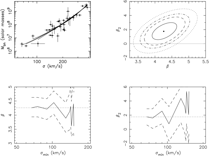
Figure 2: $\chi^{2}$ minimisation of the log-quadratic $M_{\rm bh}-\sigma$ relation. Upper Right: Contours of $\chi^{2}$ (minimised over $\alpha$) of $\beta$ and $\beta_{2}$. When projected, the contours correspond to the 1, 1.5, 2 and 2.5-sigma uncertainties on individual parameters. The point shows the most likely solution. Lower Left: The 16th, 50th (solid line) and 84th percentiles of the probability distribution for $\beta$ obtained by minimising $\chi^{2}$ as a function of the minimum $\sigma$ considered in the sample. Lower Right: The 16th, 50th (solid line) and 84th percentiles of the probability distribution for $\beta_{2}$ obtained by minimising $\chi^{2}$ as a function of the minimum $\sigma$ considered in the sample. The best fit relations for these minimum dispersions are shown in the upper-left panel, and demonstrate the effect of the lowest velocity points on the most likely fit.

4 A log-Quadratic $M_{\rm bh}-\sigma$ relation

The systematic trend of a slope that increases by 1.5-sigma when the smallest 3 of $N_{\rm g}=31$ galaxies are removed from the sample points to a fit that is systematically biased. One possibility is that a log-linear relation is not a good description of the data set. Note that a poor fit cannot be identified through a reduced value of $\chi^{2}$ that is significantly greater than unity. This is because the value of intrinsic scatter ($\epsilon_{\rm intrins}$) is determined by the condition that the reduced value of $\chi^{2}$ equal unity for the best fit solution. However we can try to find a functional form that provides a better description of the data. One possible scenario involves a characteristic velocity dispersion, with different powerlaws for large and small galaxies. To test this idea we attempt to locate a value of $\sigma$ around which the slope of the relation changes by fitting two power-law slopes, one either side of a characteristic velocity dispersion. We find that the fit is improved by allowing the slope at high $\sigma$ to be steeper than at low $\sigma$, and that the data prefers a break velocity somewhere in the range $150-350$km/s (1-sigma). Of course, while there is at least some theoretical motivation for a log-linear relation, there is no reason to suppose that the $M_{\rm bh}-\sigma$ relation should be a double power-law.

In the following we take a more general approach. As discussed in the introduction, a general relation $\log{M_{\rm bh}}=f(\log{\sigma})$ can be expanded in a Taylor series to second order yielding

$$\log(M_{\rm bh}) = \alpha+\beta\log(\sigma/200{\rm km}\,{\rm s}^{-1})$$ (4)

$$+ \beta_{2}\left[\log(\sigma/200{\rm km}\,{\rm s}^{-1})\right]^{2}.$$

Here the coefficients $\beta$ and $\beta_{2}$ represent log-linear and log-quadratic contributions to the $M_{\rm bh}-\sigma$ relation. We have (arbitrarily) expanded about $\sigma=200$km/s, which corresponds to the median velocity dispersion in the relation. The value of $\beta_{2}$ provides a measure of whether or not a log-linear relation provides a good description of the data.

We have repeated the $\chi^{2}$ minimisation using equation (4). The 1, 1.5, 2 and 2.5-sigma ellipsoids for $\beta$ and $\beta_{2}$ are shown in the upper right-hand panel of figure 2 for the Local sample. An intrinsic scatter of $\epsilon_{\rm intrins}=0.25$ dex results in a reduced $\chi^{2}$ of unity for the best fit solution. Thus a log-quadratic fit admits a slightly smaller intrinsic scatter than the log-linear relation. The solution shows evidence for a positive log-quadratic term at around the 85% level. The most likely solution has $\beta=4.3$ and $\beta_{2}=1.9$ with 1-sigma uncertainties of 0.35 and 1.1 respectively. The best fit log-quadratic relation is plotted in the upper-left panel of figure 2.

Parameter estimation using a log-linear relation corresponds to the conditional probability for $\beta$ given $\beta_{2}=0$. The horizontal grey line in the upper right panel of figure 2 shows the cut through the bi-variate probability distribution for $\beta$ and $\beta_{2}$. The contours of the bi-variate distribution cross this line centered around $\beta=4$, which is consistent with expectations from the log-linear fit. However the most probable value $\beta=4.02$ for the log-linear fit lies near the 1.5-sigma contour of the log-quadratic fit. This illustrates the point that a log-quadratic form provides a much improved description of the Local sample.

Unlike the log-linear case, the four galaxies with the lowest dispersions do not have a large influence on the log-quadratic fit. Figure 2 shows that the estimates of $\beta$ and $\beta_{2}$ do not vary systematically as the galaxies with the lowest velocity dispersions are removed from the sample. The most likely solution is similar for samples including all galaxies and for samples including only the largest 20 galaxies, indicating that there is evidence for a log-quadratic term in the main group of massive galaxies, and that the deviation from a power-law is not dominated by inclusion of low mass galaxies in the sample. The variation of the best-fit relation as small galaxies are removed from the sample may be seen visually in the left panel of figure 2, where the best-fit relations are plotted over the corresponding ranges of velocity dispersion.

The above discussion relates to an expansion of the general relation $\log{M_{\rm bh}}=f(\log{\sigma})$ which is truncated at second order. We found that the data prefers a non-zero contribution from a quadratic term. Before continuing we mention the possibility of a non-zero contribution from an additional log-cubic term. We have repeated the above analysis for the third order relation

$$\log(M_{\rm bh})=\alpha + \beta\log(\sigma/200{\rm km}\,{\rm s}^{-1})$$ (5)

$$+ \beta_{2}\left[\log(\sigma/200{\rm km}\,{\rm s}^{-1})\right]^{2}$$

$$+ \beta_{3}\left[\log(\sigma/200{\rm km}\,{\rm s}^{-1})\right]^{3}.$$

By minimising $\chi^{2}$ over the other parameters, we find a solution $\beta=4.33\pm 0.6$, $\beta_{2}=1.85\pm 2.0$ and $\beta_{3}=0.3\pm 6.0$. Not surprisingly there is a large correlation between the odd terms $\beta$ and $\beta_{3}$. This correlation increases the uncertainties on individual parameters. Despite having an additional free parameter, the log-cubic relation requires a larger intrinsic scatter to achieve a $\chi^{2}$ of unity than the log-quadratic relation. Moreover there is no evidence from the $\chi^{2}$ minimization for a log-cubic term in the Local sample. Therefore in the remainder of the paper we restrict our attention to the log-quadratic form for the $M_{\rm bh}-\sigma$ relation.

5 Choice of SMBH sample and definition of $\sigma$

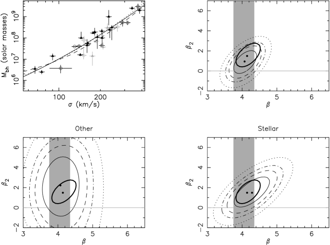
Figure 3: The upper left panel shows the Local sample with SMBH mass plotted vs effective velocity dispersion (T02). The triangles and open circles represent SMBH masses determined via stellar dynamics and by other methods (masers, gas-disks, stellar proper motions) respectively. The grey symbols denote SMBHs whose mass estimates were deemed unreliable, or whose sphere of influence was not resolved (Marconi & Hunt 2003). Log-quadratic fits were performed on three samples. In the upper right panel we show a fit to the 24 galaxies whose spheres of influence are resolved, and whose masses are deemed reliable. In the lower right panel we show a fit to the 20 galaxies with SMBH masses determined via stellar dynamics. In the lower left panel we show a fit to 11 galaxies with masses determined from methods other than stellar dynamics. Projections of the contours represent the 1, 1.5, 2 and 2.5-sigma uncertainties on individual parameters. The 1-sigma error ellipse (thick line) for the full Local sample is shown superimposed on all three panels. The grey region shows the corresponding linear fit value for $\beta$ from T02. In the upper left panel we show the three best fits.

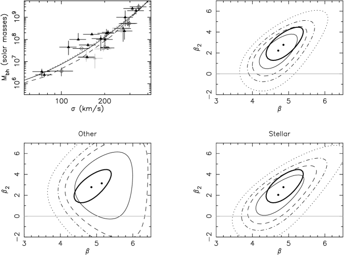
Figure 4: The upper left panel shows the Local sample with SMBH mass plotted vs central velocity dispersion (Ferrarese & Merritt 2000). The triangles and open circles represent SMBH masses determined via stellar dynamics and by other methods (masers, gas-disks, stellar proper motions) respectively. The grey symbols denote SMBHs whose mass estimates were deemed unreliable, or whose sphere of influence was not resolved (Marconi & Hunt 2003). Log-quadratic fits were performed on three samples. In the upper right panel we show a fit to the 24 galaxies whose spheres of influence are resolved, and whose masses are deemed reliable. In the lower right panel we show a fit to the 20 galaxies with SMBH masses determined via stellar dynamics. In the lower left panel we show a fit to 11 galaxies with masses determined from methods other than stellar dynamics. Projections of the contours represent the 1, 1.5, 2 and 2.5-sigma uncertainties on individual parameters. The 1-sigma error ellipse (thick line) for the full Local sample is shown superimposed on all three panels. In the upper left panel we show the three best fits.

The Local SMBH sample described in T02 contains galaxies with SMBH mass estimates obtained from data that did not resolve the sphere of influence (e.g. Marconi & Hunt 2003), and the accuracy of these masses has been called into question (e.g. Merritt & Ferrarese 2001; Ferrarese & Ford 2004; Marconi & Hunt 2003). In addition, the sample has SMBHs with masses inferred using four separate techniques, including stellar dynamics, stellar proper motions, astrophysical masers and dynamics of gaseous disks. Moreover, adding to this inhomogeneity are the different definitions for the velocity dispersion that have been supported by different groups. In this section we investigate the effect that these properties of the sample may have on the conclusion of a log-quadratic $M_{\rm bh}-\sigma$ relation. These issues are also discussed further in two appendices (§ A and B).

Some of the original SMBH mass estimates based on ground based stellar dynamical data (Magorrian et al. 1998) lie systematically above the $M_{\rm bh}-\sigma$ relation defined by other galaxies in the local sample with more secure mass estimates by as much as 2 orders of magnitude (Ferrarese & Merritt 2000). The correlation between the offset and the galaxies distance has been interpreted as evidence that the lack of resolution in these early observations resulted in a systematic resolution dependent error in the Magorrian et al. (1998) masses (Merritt & Ferrarese 2001). Of course it is not clear that one can assume masses to be incorrect because they don’t agree with the log-linear $M_{\rm bh}-\sigma$ relation as described by the remaining SMBHs. This would require the argument that the observational mass estimates must be wrong because they disagree with the a theoretical preconception that the $M_{\rm bh}-\sigma$ relation is log-linear. However concern has been expressed that that SMBH masses estimated using data that does not resolve the sphere of influence are unreliable (e.g. Ferrarese & Ford 2004). Marconi & Hunt (2003) have ordered the SMBH sample in terms of the degree to which the SMBH sphere of influence is resolved. There are 4 galaxies for which the sphere of influence is smaller than the resolution (the half-width-at-half-maximum) of the data. In addition, Marconi & Hunt (2003) classed some of the mass estimates as unreliable for other reasons such as unknown disk inclination, resulting in the removal of a further 3 galaxies from the sample. In the upper left panel of Figure 3 we show the remaining 24 galaxies (dark points). Those SMBH masses designated by Marconi & Hunt (2003) as being unreliable, and those with spheres of influence that are not resolved are plotted in grey. In the right panel of Figure 3 we show the log-quadratic fit to these 24 galaxies. The result should be compared with the fit to the full sample, the 1-sigma error ellipse for which is also plotted (thick contour). We see that the removal of the 7 unreliable galaxies has slightly increased the allowed range of $\beta_{2}$. However the solution still prefers a non-linear term, the 1-sigma error ellipse lies near the $\beta_{2}=0$ line.

In the lower right- and lower-left panels of Figure 3 we show the log-quadratic fits to the sample of galaxies with SMBH masses determined via stellar dynamics, and by other methods respectively. Each of these samples also shows evidence for a non-linear contribution to the $M_{\rm bh}-\sigma$ relation. The sample containing SMBHs with resolved spheres of influence, and the sample containing only SMBHs with masses determined via stellar dynamics have very similar solutions, indicating that SMBHs with masses determined via stellar dynamics in cases where the sphere of influence is unresolved do not skew the analysis and may be included in the sample.

The question of the dependence of resolution on the accuracy of the SMBH mass determined was investigated by Gebhardt et al. (2003). They re-evaluated the SMBH masses for galaxies where the SMBH mass had been previously determined with ground-based imaging using higher resolution space-based data. Gebhardt et al. (2003) showed that i) the Magorrian et al. (1998) masses were indeed overestimated, by up to a factor of 3, due to the assumption of 2-integral models; and ii) comparison of 3-integral modeling of low-resolution ground based and high resolution space based data demonstrates that the SMBH mass determinations described in Gebhardt et al. (2003) contain no resolution induced bias. In other words, provided that the modeling is sufficiently general, the high resolution data increases the precision but not the accuracy of SMBH mass estimates (see figure 8 of Gebhardt et al. 2003). This implies that if the resolution were not sufficient, then the lower limit on BH mass would be $<0$ (i.e. no definite detection). Thus the effect of spatial resolution is built into the estimate of the range of allowable mass. The masses of SMBHs in galaxies where the sphere of influence is not resolved should therefore be just as reliable as those where it is resolved, in the sense that the determination is just as accurate but carries less precision (Richstone et al. 2004).

At this point it should be noted that recent work from Valluri, Merritt & Emsellem (2004) has suggested that stellar dynamical estimates of SMBH masses are unreliable even when the SMBH sphere of influence is resolved. This unreliability is due to a degeneracy between the mass-to-light ratio and SMBH mass, which was shown to become more prominent as the number of orbits used in the modeling is increased. On the other hand, Richstone et al. (2004) have countered this claim. They suggest that while it is true that the allowed range of SMBH mass increases with the number of orbits assumed, this range asymptotes to provide a true estimate of SMBH mass. Thus they conclude that provided the number of orbits is sufficient, SMBH mass estimation from reconstruction of stellar orbits using kinematic data can lead to a robust SMBH mass estimate. Richstone et al. (2004) estimate the number of orbits that are required to achieve convergence in the mass estimate and conclude that published mass estimates have been made using a sufficiently large orbit library and are therefore reliable.

Finally, the definition of the independent variable may be an important factor in the evaluation of any non-linear contribution to the $M_{\rm bh}-\sigma$ relation. A central velocity dispersion has been advocated by Ferrarese & Merritt (2001), while an effective velocity dispersion was used by Gebhardt et al. (2000). The pros and cons of these different variables were summarised by Merritt & Ferrarese (2001). The central velocity dispersion is more easily measured than the effective velocity dispersion which requires both surface photometry and spatially resolved spectroscopy over the effective radius of the galaxy. As a result, central velocity dispersions have been measured for many galaxies, while the effective velocity dispersions require significant effort to obtain the required data. On the other hand the effective velocity dispersion better represents the velocity dispersion over the stellar spheroid, and may therefore be expected to offer a better representation of the depth of the spheroids gravitational potential well. Moreover T02 found that the SMBH itself could effect the value of the central velocity by up to 30% in some cases. In order to evaluate the effect of changing the independent variable from an effective to a central velocity dispersion, we repeat the above analysis on sub-samples of the Local sample of SMBHs (values of central velocity dispersion are available in Merritt & Ferrarese 2001 & Ferrarese & Ford 2004). The results are shown in Figure 4, correspond to, and are qualitatively similar to to those in Figure 3, where the effective velocity dispersion was the independent variable. In particular, if the SMBHs whose spheres of influence are not resolved are removed from the sample, then the sample still prefers a non-linear contribution. This non-linearity is at higher significance where the central rather than effective velocity dispersion is used. Similarly, samples of SMBHs with masses determined via stellar dynamics and by other methods each prefer a non-linear $M_{\rm bh}-\sigma$ relation. This analysis shows the previously known result that use of the central velocity dispersion results in an estimate of the $M_{\rm bh}-\sigma$ relation that is steeper than where the effective velocity dispersion is used.

In summary, samples where the SMBH masses were estimated by stellar dynamics, samples where the SMBH masses were determined via other methods, and samples where the SMBH masses are secure (Marconi & Hunt 2003), each have a fit that prefers the inclusion of a log-quadratic term. The sample of SMBH masses determined via other methods shows the strongest non-linear tendency, but with the largest uncertainty. This non-linear component of the $M_{\rm bh}-\sigma$ relation is present whether the independent variable is considered to be the central velocity dispersion (Ferrarese & Merritt 2000) or the effective velocity dispersion (T02). In light of these results, we consider only the full Local sample as described in T02, with the effective velocity dispersion as the independent variable, in the remainder of this paper.

6 Bayesian Parameter Estimation

Our aim in this paper is to determine the parameters $\alpha$, $\beta$ and $\beta_{2}$, as well as the intrinsic scatter (designated $\delta$) of SMBHs around equation (4). Our general approach adds two features relative to the $\chi^{2}$ analysis described in the previous sections. First, our approach explicitly includes the intrinsic scatter (labeled $\delta$) about the mean $M_{\rm bh}-\sigma$ relation as a third free parameter, and we consistently solve for all of $\alpha$, $\beta$, $\beta_{2}$ and $\delta$. The second improvement is to include the asymmetric errors quoted for $M_{\rm bh}$.

In the absence of errors in $M_{\rm bh}$ and $\sigma$ we may define the contribution $LH_{i}$ of SMBH $i$ to the likelihood $LH_{\alpha,\beta,\beta_{2},\delta}$ for the set $\{\alpha,\beta,\beta_{2},\delta\}$. However both $M_{\rm bh}$ and $\sigma$ contain observational uncertainty. Each of the $LH_{i}$ must therefore be averaged over the uncertainty in both $M_{\rm bh}$ and $\sigma$, hence

$$LH_{i} \equiv \int_{-\infty}^{\infty}d\log{\sigma}\frac{dP_{i}}{d\log{\sigma}}\int_{-\infty}^{\infty}d\log{M_{\rm bh}}$$ (6)

$$\hskip 85.35826pt\frac{dP_{i}}{d\log{M_{\rm bh}}}LH(\sigma,M_{\rm bh}).$$

The uncertainty in $\sigma$ is described by $dP_{i}/d\log{\sigma}=N(d\log{\sigma_{i}},0.02)$ for all galaxies except the Milky-Way for which, following T02 we assume a larger uncertainty, $dP_{i}/d\log{\sigma}=N(d\log{\sigma_{i}},0.08)$. Here the notation $N(x|\bar{x},\delta x)$ refers to the value of a Gaussian distribution with mean $\bar{x}$ and variance $\delta x$ at $x$. The observed uncertainty in $M_{{\rm bh},i}$ is assumed to follow a distribution

$$\frac{dP_{i}}{d\log{M_{\rm bh}}} = N(\log{M_{\rm bh}}|\log{M_{{\rm bh},i}},\Delta\log{M^{\rm low}_{{\rm bh},i}})$$ (7)

$$\hskip 93.89409pt\mbox{if}\hskip 8.53581ptM_{{\rm bh}}<M_{{\rm bh},i}$$

$$= N(\log{M_{\rm bh}}|\log{M_{{\rm bh},i}},\Delta\log{M^{\rm upp}_{{\rm bh},i}})$$

$$\hskip 93.89409pt\mbox{if}\hskip 8.53581ptM_{{\rm bh}}\geq M_{{\rm bh},i}$$

Here we have defined $\Delta\log{M^{\rm upp}_{\rm bh,i}}$ and $\Delta\log{M^{\rm low}_{\rm bh,i}}$ as the uncertainty (in dex) above and below the observed value for SMBH $i$. The values of $\alpha$, $\beta$, $\beta_{2}$ and $\delta$ may then be estimated by maximising the product of likeli-hoods for the $N_{\rm g}$ residuals

$$LH_{\alpha,\beta,\beta_{2},\delta}=\Pi_{i=0}^{N_{\rm g}}LH_{i}$$

Note that we have not yet specified the definition of $LH(\sigma,M_{\rm bh})$. For a finite sample size, the solution for $\alpha$, $\beta$, $\beta_{2}$ and $\delta$ is sensitive to the definition of $LH(\sigma,M_{\rm bh})$. As a result, an inappropriate choice for $LH(\sigma,M_{\rm bh})$ can lead to a biased estimate of the parameters. In this paper we are analysing a sample where SMBH mass is unbiased at a fixed value of $\sigma$. We therefore treat $\sigma$ as the independent variable and model the intrinsic scatter as a Gaussian with variance $\delta$, hence

$$LH(\sigma,M_{\rm bh}) \equiv N(\Delta_{M_{\rm bh},i}|0,\delta)$$ (8)

$$\mbox{where}\hskip 14.22636pt\Delta_{M_{\rm bh},i}=\log{M_{{\rm bh},i}}-\left[\alpha+\beta\log{\left(\frac{\sigma_{i}}{200\mbox{km/s}}\right)}\right.$$

$$\hskip 56.9055pt\left.+\beta_{2}\log{\left(\frac{\sigma_{i}}{200\mbox{km/s}}\right)^{2}}\right].$$

Figure 5: The cumulative distribution of maximum likelihood solutions for the inferred values of $\beta_{\rm infer}$ and $\beta_{\rm 2,infer}$ in Monte-Carlo samples given different input values $\beta_{\rm true}$ and $\beta_{\rm 2,true}$, which are shown by the vertical solid lines. The dots and dashed lines show the distribution means and medians respectively. Upper panels: The input relation had $\beta_{\rm true}=4.2$ and $\beta_{\rm 2,true}=1.6$. The dashed lines show the 16th and 84th percentiles. Lower panels: The input relation had $\beta_{\rm true}=4.02$ and $\beta_{\rm 2,true}=0.$ The dot-dashed lines show the values of $\beta$ and $\beta_{2}$ inferred from the data.

The joint a-posteriori probability distributions for the parameters $\alpha$, $\beta$ , $\beta_{2}$ and $\delta$ may be found from

$$\frac{d^{4}P}{d\alpha d\beta d\beta_{2}d\delta}\propto LH_{\alpha,\beta,\beta_{2},\delta}\frac{dP_{\rm prior}}{d\alpha}\frac{dP_{\rm prior}}{d\beta}\frac{dP_{\rm prior}}{d\beta_{2}}\frac{dP_{\rm prior}}{d\delta},$$ (9)

where the $P_{\rm prior}$ are prior probabilities, which we assume to be flat in this paper, i.e.

$$\frac{dP_{\rm prior}}{d\alpha}\propto\frac{dP_{\rm prior}}{d\beta}\propto\frac{dP_{\rm prior}}{d\beta_{2}}\propto\frac{dP_{\rm prior}}{d\delta}\propto 1.$$ (10)

A-posteriori distributions for combinations of these parameters may then be obtained by marginalising over the other dimensions, for example

$$\frac{d^{2}P}{d\delta d\beta}\propto\int_{-\infty}^{\infty}d\alpha\int_{-\infty}^{\infty}d\beta_{2}\frac{d^{4}P}{d\alpha d\beta d\beta_{2}d\delta}$$ (11)

or

$$\frac{dP}{d\beta}\propto\int_{-\infty}^{\infty}d\alpha\int_{-\infty}^{\infty}d\beta_{2}\int_{0}^{\infty}d\delta\frac{d^{4}P}{d\alpha d\beta d\beta_{2}d\delta}.$$ (12)

6.1 Bias in Parameter Estimation

Before presenting the probability distributions for the parameters $\beta$, $\beta_{2}$ and $\delta$ that describe the Local sample, we asses the bias in the fitting procedure by fitting parameters to Monte-Carlo realisations of mock SMBH samples. We generate samples of $N_{\rm g}=31$ SMBHs using the following procedure. For each of the $N_{\rm g}=31$ galaxies we select a value of $\sigma$ drawn from the observed estimate $N(\sigma_{i},\Delta\sigma_{i})$. This value is used to select a SMBH mass from an input mean relation, offset randomly according to the input intrinsic scatter $\delta_{\rm true}$. This mass is then further offset by a value drawn randomly from the quoted uncertainty in $M_{\rm bh}$ for the corresponding SMBH in the observed sample. We assumed input values of $\beta_{\rm true}=4.2$ and $\beta_{\rm 2,true}=1.6$. In the following section we show that these values lie near the best fit relation for the Local sample. The intrinsic scatter of the relations was assumed to be $\delta_{\rm true}=0.3$, defined in the $y$ or $M_{\rm bh}$ direction.

For each mock sample we find the most likely values for $\beta$ and $\beta_{2}$ from equation (9). The cumulative distributions of the best fit solutions are plotted in the upper panels of figure 5. The estimates are not skewed, but the parameters determined are slightly biased (by $\delta\beta=0.1$ and $\delta\beta_{2}=0.2$) as may be seen by the comparing the median (dashed line) and mean (denoted by the large dot) to the true value (solid vertical line) in each case.

7 Unbiased A-posteriori probability distributions for parameters in the log-quadratic $M_{\rm bh}-\sigma$ Relation

Having assessed the bias in our parameter estimation, we are in a position to estimate the parameters describing the Local sample. In figure 6 we show the a-posteriori marginalised probability distributions for the parameters $\beta$, $\beta_{2}$ and $\delta$ computed using equations (11-12) in combination with the likelihood equation (8). The values of $\beta$ and $\beta_{2}$ corresponding to a fixed likelihood have been corrected a-posteriori for the biases $\Delta\beta=0.1$ and $\Delta\beta_{2}=0.2$. In the central row we show joint distributions for $\beta_{2}$ and $\beta$ (left) and for $\delta$ and $\beta$ (right). The contours (dark lines) refer to 0.036, 0.14, 0.26 and 0.64 of the peak height corresponding to the 4, 3, 2, and 1-sigma limits of a Gaussian distribution. In the bottom rows (dark lines) we show differential (solid lines) and cumulative (dashed lines) distributions for $\beta$ (left) and $\beta_{2}$ (right). The vertical dotted lines show the variance.

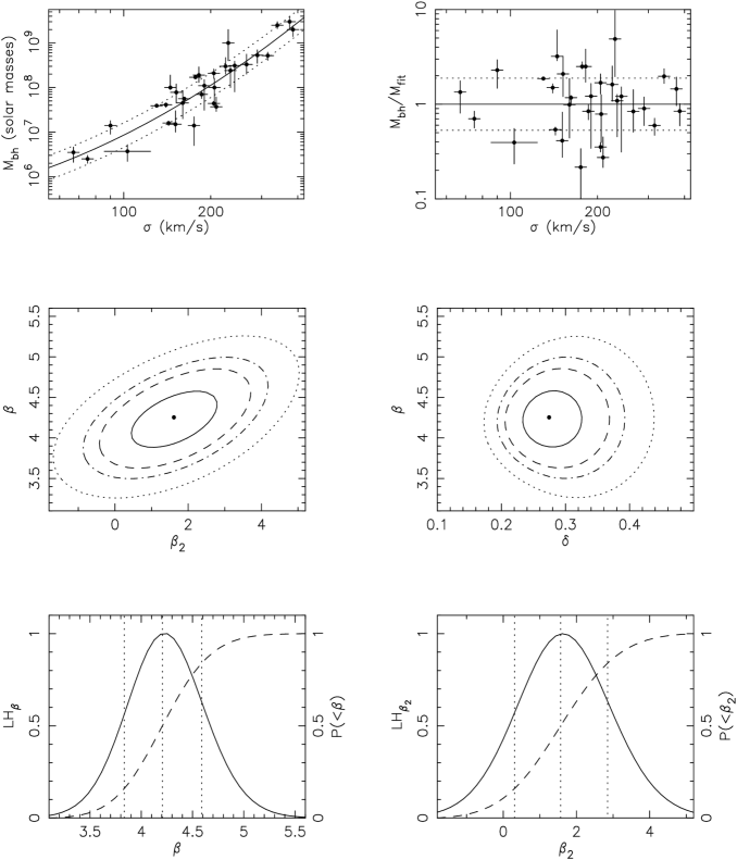
Figure 6: Upper Left: SMBH mass vs. central velocity dispersion from the compilation of T02. The solid line shows the best fit solution to equation (4) obtained using a likelihood defined in equation (8). The dotted lines show the level of intrinsic scatter around the best-fit relation. Upper Right: Residuals relative to the maximum likeli-hood solution. The dotted lines show the best fit value of intrinsic scatter. The lower panels show the a-posteriori probability distributions for the parameters $\beta$, $\beta_{2}$ and $\delta$. Center Left: Joint distribution for $\beta$ and $\beta_{2}$ marginalised over $\alpha$ and $\delta$. Center Right: Joint distribution for $\delta$ and $\beta$ marginalised over $\alpha$ and $\beta_{2}$. The contours refer to 0.036, 0.14, 0.26 and 0.64 of the peak height corresponding to the 4, 3, 2, and 1-sigma limits of a Gaussian distribution. Bottom Left: Differential (solid line) and cumulative (dashed line) distributions for $\beta$ marginalised over $\beta_{2}$, $\delta$ and $\alpha$. Bottom Right: Differential (solid line) and cumulative (dashed line) distributions for $\beta_{2}$ marginalised over $\beta$, $\delta$ and $\alpha$. The vertical dotted lines show the 16th, 50th and 84th percentiles.

The contours show little correlation between parameters. Using the likelihood defined in equation (8) we find that the marginalised distributions imply $\beta=4.2\pm 0.37$ and $\beta_{2}=1.6\pm 1.3$ (figure 6), and an intrinsic scatter of $\delta=0.28\pm 0.04$. The normalisation was found to be $\alpha=8.05\pm 0.06$. The best fit (solid line) is plotted over the data in the upper left panel of figure 6, together with curves showing the level of intrinsic scatter (dotted lines). In the upper right panel of figure 6 we plot the residuals in $\log{M_{\rm bh}}$, together with horizontal dotted lines showing the value of the best fit intrinsic scatter. We have assumed an intrinsic scatter that is constant with $\sigma$. Inspection of the residuals in figure 6 indicates that there is no systematic trend.

The cumulative probability distribution for $\beta_{2}$ shows that there is a positive contribution (at $90\%$ confidence) from a log-quadratic term in the $M_{\rm bh}-\sigma$ relation that describes the Local sample. This may be interpreted as indicating that at the 80% level the $M_{\rm bh}-\sigma$ relation does not follow a single powerlaw between $\sim 70$km/s and $\sim 380$km/s. An alternative statistical question regarding the significance of this result concerns the frequency with which one might measure a log-quadratic term as large as the best fit of $\beta_{2}=1.6$, assuming an intrinsically log-linear relation. We have performed fits to mock samples assuming an input intrinsic slope of $\beta_{\rm true}=4.02$ and an input $\beta_{\rm 2,true}=0$, which corresponds to the best fit log-linear relation (T02). The cumulative distributions for the best fit $\beta$ and $\beta_{2}$ are plotted in the lower panels of figure 5. We find that the estimate of $\beta$ is unbiased in this case, and that the best fit value of $\beta_{2}$ is greater than 1.6 around $10\%$ of the time. This is consistent with the statement that the Local sample does not follow a single power-law at the $\sim 80\%$ level.

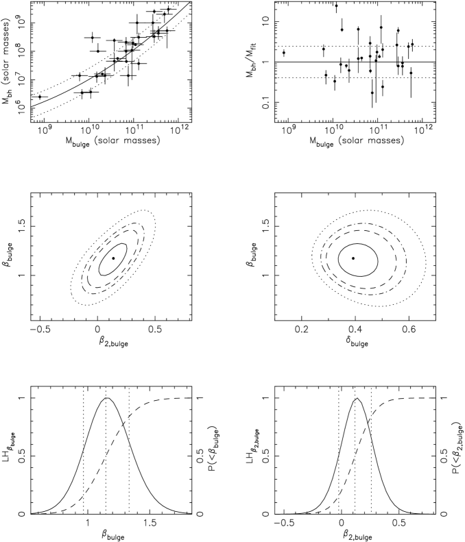
Figure 7: Upper Left: SMBH mass vs. bulge mass from the compilation of Haering & Rix (2004). The solid line shows the best fit solution to equation (13) obtained using a likelihood defined in equation (15). The dotted lines show the level of intrinsic scatter around the best-fit relation. Upper Right: Residuals relative to the maximum likeli-hood solution. The dotted lines show the best fit value of intrinsic scatter. The lower panels show the a-posteriori probability distributions for the parameters $\beta_{\rm bulge}$, $\beta_{\rm 2,bulge}$ and $\delta_{\rm bulge}$. Center Left: Joint distribution for $\beta_{\rm bulge}$ and $\beta_{\rm 2,bulge}$ marginalised over $\alpha_{\rm bulge}$ and $\delta_{\rm bulge}$. Center Right: Joint distribution for $\delta_{\rm bulge}$ and $\beta_{\rm bulge}$ marginalised over $\alpha_{\rm bulge}$ and $\beta_{\rm 2,bulge}$. The contours refer to 0.036, 0.14, 0.26 and 0.64 of the peak height corresponding to the 4, 3, 2, and 1-sigma limits of a Gaussian distribution. Bottom Left: Differential (solid line) and cumulative (dashed line) distributions for $\beta_{\rm bulge}$ marginalised over $\beta_{\rm 2,bulge}$, $\delta_{\rm bulge}$ and $\alpha_{\rm bulge}$. Bottom Right: Differential (solid line) and cumulative (dashed line) distributions for $\beta_{\rm 2,bulge}$ marginalised over $\beta$, $\delta$ and $\alpha$. The vertical dotted lines show the 16th, 50th and 84th percentiles.

The inclusion of a log-quadratic term in the fit leads to residuals that do not lie systematically above the mean relation at high or low $\sigma$. We can therefore use the behaviour of these residuals to interpret the significance of the log-quadratic term. Our Monte-Carlo simulations (figure 5) show that (after accounting for the bias) $\sim 10\%$ of samples with $\beta=4.2$ and $\beta_{2}=1.6$ produce best fits with $\beta_{2}<0$. As we saw in figure 1 the smallest three galaxies all have SMBHs that are more massive than the average implied by a log-linear fit. Each SMBH has $\sim 1$ chance in 2 of lying above the mean relation. This situation would therefore arise by chance for $\sim 1$ sample in 10 ($\sim 1/2^{3}$), which provides an intuitive understanding of the finding that there is a log-quadratic term in the $M_{\rm bh}-\sigma$ relation described by the Local sample that is positive at the 90% level.

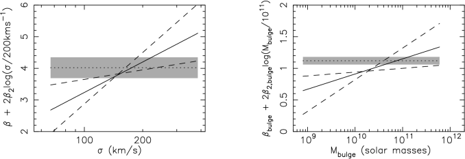
Figure 8: The values of logarithmic slope for the mean relations (solid lines) and for the relations using parameters on the edge of the 1-sigma error ellipses that lead to the most extreme examples (dashed lines). The logarithmic slopes are shown as a function of $\sigma$ for the $M_{\rm bh}-\sigma$ (left panel) and $M_{\rm bh}-M_{\rm bulge}$ relations (right panel). The grey regions represent the 1-sigma ranges for $\beta$ (T02) and $\beta_{\rm bulge}$ (Haering & Rix 2004) using a log-linear relation.

8 The log-quadratic $M_{\rm bh}-M_{\rm bulge}$ Relation

In this section we apply our analysis to the sample of SMBHs and bulge masses summarised in Haering & Rix (2004). This sample closely resembles that described in T02. The SMBH-bulge mass relation is shown in the upper left panel of figure 7, and can be described by a log-quadratic relation of the form

$$\log(M_{\rm bh})=\alpha_{\rm bulge} + \beta_{\rm bulge}\log(M_{\rm bulge}/10^{11}M_{\odot})$$ (13)

$$+ \beta_{\rm 2,bulge}\left[\log(M_{\rm bh}/10^{11}M_{\odot})\right]^{2}.$$

We have repeated our $\chi^{2}$ analysis on the $M_{\rm bh}-M_{\rm bulge}$ sample (not shown). We find that the slope estimated using a log-linear fit systematically increases by an amount that is greater than the statistical uncertainty when the smallest galaxies are removed from the sample. A $\chi^{2}$ minimisation of a log-quadratic relation provides a significantly better fit, with the power-law relation ruled out at the 1-sigma level. The parameters of the log-quadratic fit do not vary systematically as galaxies are removed from the sample.

Motivated by the success of the log-quadratic fit for the $M_{\rm bh}-M_{\rm bulge}$ relation in a $\chi^{2}$ minimisation, we perform a Bayesian analysis in analogy to the one described in the previous section. We define a likeli-hood function

$$LH_{i} \equiv \int_{-\infty}^{\infty}d\log{M_{\rm bulge}}\frac{dP_{i}}{d\log{M_{\rm bulge}}}\int_{-\infty}^{\infty}d\log{M_{\rm bh}}$$ (14)

$$\hskip 56.9055pt\frac{dP_{i}}{d\log{M_{\rm bh}}}LH(M_{\rm bulge},M_{\rm bh}),$$

where $LH(M_{\rm bulge},M_{\rm bh})$ is the likelihood of a set of $M_{\rm bulge}$ and $M_{\rm bh}$ given a relation described by $\alpha_{\rm bulge}$, $\beta_{\rm bulge}$, $\beta_{\rm 2,bulge}$ and $\delta_{\rm bulge}$. Following Haering & Rix (2004) the uncertainty in $M_{\rm bulge}$ is described by $dP_{i}/d\log{M_{\rm bulge}}=N(d\log{M_{\rm bulge}},0.18)$ for all galaxies. At fixed bulge mass, we model the intrinsic scatter as a Gaussian with variance $\delta_{\rm bulge}$, hence we define a likeli-hood in analogy with equation (8)

$$LH(M_{\rm bulge},M_{\rm bh}) \equiv N(\Delta_{M_{\rm bh},i}|0,\delta_{\rm bulge})$$ (15)

$$\mbox{where}\hskip 8.53581pt\Delta_{M_{\rm bh},i}=\log{M_{{\rm bh},i}}$$

$$-\left[\alpha_{\rm bulge}+\beta_{\rm bulge}\log{\left(\frac{M_{{\rm bulge},i}}{5\times 10^{10}M_{\odot}}\right)}\right.$$

$$\left.+\beta_{\rm 2,bulge}\left[\log{\left(\frac{M_{{\rm bulge},i}}{5\times 10^{10}M_{\odot}}\right)}\right]^{2}\right].$$

We performed Monte-Carlo simulations as before and find that the estimator described in equation (15) leads to a slightly biased estimate for the true values $\beta_{\rm bulge,true}$ and $\beta_{\rm 2,bulge,true}$. We find biases of $\Delta\beta_{\rm bulge}=0.04$ and $\Delta\beta_{\rm 2,bulge}=0.035$.

In figure 7 we show the a-posteriori marginalised probability distributions for the parameters $\beta_{\rm bulge}$, $\beta_{\rm 2,bulge}$ and $\delta_{\rm bulge}$ computed using the likelihood equation (15) and corrected for bias. In the central row we show joint distributions for $\beta_{\rm 2,bulge}$ and $\beta_{\rm bulge}$ (left) and for $\delta_{\rm bulge}$ and $\beta_{\rm bulge}$ (right). The contours (dark lines) refer to 0.036, 0.14, 0.26 and 0.64 of the peak height corresponding to the 4, 3, 2, and 1-sigma limits of a Gaussian distribution. In the bottom rows we show differential (solid lines) and cumulative (dashed lines) distributions for $\beta_{\rm bulge}$ (left) and $\beta_{\rm 2,bulge}$ (right). The vertical dotted lines show the variance. We find that the marginalised distributions imply $\beta_{\rm bulge}=1.15\pm 0.19$, $\beta_{\rm 2,bulge}=0.12\pm 0.14$ and an intrinsic scatter of $\delta=0.41\pm 0.07$. The normalisation is $\alpha_{\rm bulge}=8.05\pm 0.1$. The best fit relation has a positive log-quadratic term. However this term is only required by the data at the 1-sigma level. Haering & Rix (2004) suggested an upper limit on the intrinsic scatter of $\sim 0.3$ dex, though the definition of this scatter was not specified. We have included intrinsic scatter self consistently in the analysis and find that the intrinsic scatter in SMBH mass at fixed bulge mass is $\delta_{\rm bulge}\sim 0.4$ dex. This scatter is larger than the quoted uncertainties on either SMBH or bulge mass. The scatter in the $M_{\rm bh}-M_{\rm bulge}$ relation is also $\sim$50% larger than the scatter in the $M_{\rm bh}-\sigma$ relation.

The best fit log-quadratic relation is plotted over the data (solid line) in the upper left panel of figure 7 together with curves showing the level of intrinsic scatter (dotted lines). In the upper right panel of figure 7 we plot the resulting residuals, together with horizontal dotted lines showing the value of the best fit intrinsic scatter. Inspection of the residuals does not indicate any systematic trend of residuals as a function of $M_{\rm bulge}$.

9 Discussion

To quantify the extent of the departure of the Local sample from a log-linear relation we have plotted the logarithmic derivatives $d\log{M_{\rm bh}}/d\log{\sigma}$ and $d\log{M_{\rm bh}}/d\log{M_{\rm bulge}}$ of the $M_{\rm bh}-\sigma$ and $M_{\rm bh}-M_{\rm bulge}$ relations as a function of $\sigma$ and $M_{\rm bulge}$ in figure 8. The solid lines show the slopes of the best fit relations. The dashed lines show the slope of relations at the edges of the 1-sigma error ellipsoids in $\beta-\beta_{2}$ (left panel) or $\beta_{\rm bulge}-\beta_{\rm 2,bulge}$ (right panel) space, while the grey stripes show the 1-sigma range for the slope of the log-linear fits from T02 and Haering & Rix (2004) respectively. The figure shows that in both cases the logarithmic slope of the log-quadratic relation varies substantially more over the range of $\sigma$ or $M_{\rm bulge}$ in the SMBH sample than the statistical uncertainty in the slope $\beta$ of a log-linear fit. This fact has contributed to statistical bias and inconsistent results when comparing the log-linear slopes of the $M_{\rm bh}-\sigma$ relation between different samples of SMBHs. In the remainder of this section we discuss various implications of a log-quadratic $M_{\rm bh}-\sigma$ relation.

9.1 The most massive SMBH

The possibility of a log-quadratic $M_{\rm bh}$-$\sigma$ relation leads to several interesting consequences. The first concerns the velocity dispersion of galaxies in which the most massive SMBHs reside. The mass of the largest SMBHs in the Sloan Digital Sky Survey (SDSS) survey volume was discussed in Wyithe & Loeb (2003). We repeat part of the discussion here. Consider a SMBH of mass $M_{\rm bh}=3\times 10^{9}M_{\odot}$. We can estimate the co-moving density of black-holes of this mass from the observed quasar luminosity function and an estimate of quasar lifetime. If we assume Eddington accretion, then at the peak of quasar activity, quasars powered by $M_{\rm bh}\ga 3\times 10^{9}M_{\odot}$ SMBHs had a comoving density of $\Psi\sim 50$Gpc^-3. Wyithe & Loeb (2003) found that the number of quasars relative to the number of dark-matter halos at $z\sim 3$ implies a duty cycle for quasars of $\sim 0.005$. The comoving density of SMBHs with masses in excess of $M_{\rm bh}\sim 3\times 10^{9}M_{\odot}$ at $z\sim 3$ was therefore $\sim 10^{4}$Gpc^-3. As this corresponds to the peak of SMBH growth, the SMBH density should match the value observed today. This density implies that the nearest SMBH of $\sim 3\times 10^{9}M_{\odot}$ should be at a distance $d_{\rm bh}\sim 30$Mpc which is comparable to the distance of M87, a galaxy known to possess a SMBH of this mass (Ford et al. 1994). What is the most massive SMBH that can be detected dynamically in the SDSS? The SDSS probes a volume of $\sim 1$Gpc³ out to a distance $\sim 30$ times that of M87. At the peak of quasar activity, the density of the brightest quasars implies that there should be $\sim 100$ SMBHs with masses greater than $\sim 3\times 10^{10}M_{\odot}$ per Gpc³, the nearest of which will be at a distance $d_{\rm bh}\sim 130$Mpc, or 5 times the distance to M87. The radius of gravitational influence of the SMBH scales as $M_{\rm bh}/\sigma^{2}$. We therefore find that for the nearest $3\times 10^{9}M_{\odot}$ and $3\times 10^{10}M_{\odot}$ SMBHs, the angular radius of influence should be similar. Thus the dynamical signature of the nearest $\sim 3\times 10^{10}M_{\odot}$ SMBHs on their stellar host should be detectable.

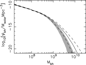
Figure 9: Mass-functions for SMBHs. Two mass functions are shown. The grey stripe and dashed lines represent the ranges of uncertainty in the estimate of the mass-function assuming the log-linear and log-quadratic relations respectively. The ranges at fixed $M_{\rm bh}$ in each case correspond to the 16th and 84th percentiles. The solid line shows the most likely estimate for the mass-function corresponding to the log-quadratic $M_{\rm bh}-\sigma$ relation.

In order to find these most massive SMBHs one needs to identify the galaxies in which they reside. We estimate the value of $\sigma$ implied for SMBHs of mass $\sim 10^{10}M_{\odot}$ using the mean $M_{\rm bh}-\sigma$ relation. If one adopts the mean log-linear relation (T02), then SMBHs with masses in excess of $10^{10}M_{\odot}$ should reside in galaxies with $\sigma\ga 600$km/s (see figure 11). However no such galaxies exist is the SDSS (e.g. Sheth et al. 2003), where largest values of galaxy velocity dispersion are found to be $\sigma\sim 400$km s^-1. The mean log-quadratic relation reaches $M_{\rm bh}\sim 10^{10}M_{\odot}$ at a more modest but still unobserved velocity dispersion, $\sigma\sim 500$km/s. However the intrinsic scatter in the $M_{\rm bh}-\sigma$ relation is $\delta\sim 0.3$ dex. We find that SMBHs of mass $\sim 10^{10}M_{\odot}$ differ by $\la 2\delta$ from the mean log-quadratic relation at $\sigma\sim 400$km/s. The most massive SMBHs with masses of $\sim 10^{10}M_{\odot}$ inferred from quasars at $z\sim 3$ should therefore exist in the SDSS and would lie at $\sim 2\delta$ above the extrapolated mean log-quadratic relation for galaxies with the largest measured velocity dispersions of $\sigma=400$km/s. This helps to reconcile the number of luminous quasars observed at $z\sim 3$ with both the local $M_{\rm bh}-\sigma$ relation and the lack of super massive galaxies.

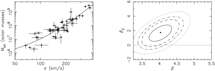
Figure 10: Left: The Local sample of SMBHs (solid dots) and the sample of SMBHs determined from reverberation mapping studies (with $\langle f_{\rm v}\rangle=5.5$; Onken et al. 2004; open circles). Right: The resulting contours of $\chi^{2}$ (minimised over $\alpha$) of $\beta$ and $\beta_{2}$. Projections of the contours correspond to the 1, 1.5, 2 and 2.5-sigma limits on individual parameters. The point shows the most likely solution.

9.2 The mass-function of SMBHs

A positive log-quadratic term has a significant effect on the upper end of the SMBH mass-function. In figure 9 we show the SMBH mass-function computed by combining the $M_{\rm bh}-\sigma$ relation with the velocity dispersion function of Sheth et al. (2003). Two mass functions are shown. The grey stripe and dashed lines represent the ranges of uncertainty in the estimate of the mass-function obtained assuming log-linear and log-quadratic $M_{\rm bh}-\sigma$ relations respectively. The ranges at fixed $M_{\rm bh}$ in each case correspond to the 16th and 84th percentiles, and were computed taking into account Gaussian uncertainties in both the parameters of the $M_{\rm bh}-\sigma$ relation and the velocity-dispersion function. The solid line shows the most likely estimate for the mass-function corresponding to the log-quadratic $M_{\rm bh}-\sigma$ relation. Figure 9 shows that inclusion of a log-quadratic term in the $M_{\rm bh}-\sigma$ relation results in an estimate for the number density of SMBHs with masses of $\sim 10^{10}M_{\odot}$ that is several orders of magnitude larger than inferred from a log-linear relation. We have estimated the mass density (for a Hubbles constant of $71$km s${}^{-1}\,$Mpc^-1) of SMBHs in the local universe. For a log-linear $M_{\rm bh}-\sigma$ relation we find a density of $\rho=(2.30\pm 0.45)\times 10^{5}M_{\odot}\,$Mpc^-3, while for a log-quadratic $M_{\rm bh}-\sigma$ relation we obtain $\rho=(2.35\pm 0.45)\times 10^{5}M_{\odot}\,$Mpc^-3. Hence the addition of a log quadratic term does not effect estimates of the total mass density which is dominated by SMBHs in the range $10^{7}-10^{9}M_{\odot}$ (Aller & Richstone 2002).

9.3 Inclusion of SMBHs from reverberation mapping studies

The sample of kinematically detected SMBHs will not grow by a large factor in the foreseeable future (Ferrarese 2003). Progress in understanding the statistical properties of the SMBH population may instead come via estimates of SMBH masses that are based on reverberation mapping studies (Gebhardt et al. 2000b; Ferrarese et al. 2001; Onken et al. 2004; Peterson et al. 2004; Nelson et al 2004). Onken et al. (2004) have presented a sample of 14 SMBHs with virial masses ($M_{\rm bh,vir}$) determined via reverberation mapping studies, in galaxies with measured velocity dispersions. Reverberation masses are determined up to a geometric factor $f$, hence the SMBH mass is $M_{\rm bh}=f\times M_{\rm bh,vir}$. Onken et al. (2004) have determined the average value $\langle f\rangle$ by comparing the reverberation masses of these 14 SMBHs, to the masses of SMBHs in the Local sample using a log-linear $M_{\rm bh}-\sigma$ relation. They found $\langle f\rangle\sim 5.5$ over a range of values for the slope $\beta$ that include $\beta=4.58$ (Ferrarese 2002) and $\beta=4.02$ (T02). Assuming this scaling factor we can combine the 14 galaxies used to obtain $\langle f\rangle$ in Onken et al. (2004) with the Local sample of SMBHs to form a sample of 45 galaxies.

The left panel of figure 10 shows the $M_{\rm bh}-\sigma$ relation for the Local sample (solid dots), and its comparison to the AGN SMBH masses and velocity dispersions (open circles) presented in Onken et al. (2004). We have repeated the $\chi^{2}$ minimisation using equation (4) for the combined sample of $N_{\rm g}=45$ SMBHs. In the right-hand panel we show the 1, 1.5, 2 and 2.5-sigma ellipsoids for $\beta$ and $\beta_{2}$. The most likely solution has $\beta=4.05$ and $\beta_{2}=1.8$ with 1-sigma uncertainties of 0.3 and 1.0 respectively. The resulting best-fit $M_{\rm bh}-\sigma$ relation is over-plotted in the left panel (solid line). This solution is very close to the one obtained using only SMBHs in the Local sample ($\beta=4.3\pm 0.35$, $\beta_{2}=1.9\pm 1.4$). The intrinsic scatter required for a reduced $\chi^{2}$ of unity in this fit was $\epsilon_{\rm intrins}=0.25$ dex, indicating that the addition of the AGN SMBHs does not increase the scatter of the $M_{\rm bh}-\sigma$ relation. The addition of AGN SMBHs results in a fit with a log-quadratic term which is non-zero at around the 1.5-sigma level. The sample of AGN SMBHs with masses determined from reverberation mapping therefore strongly supports a log-quadratic $M_{\rm bh}-\sigma$ relation. This is despite the fact that the normalization of the reverberation SMBH masses was determined via the assumption of a log-linear relation.

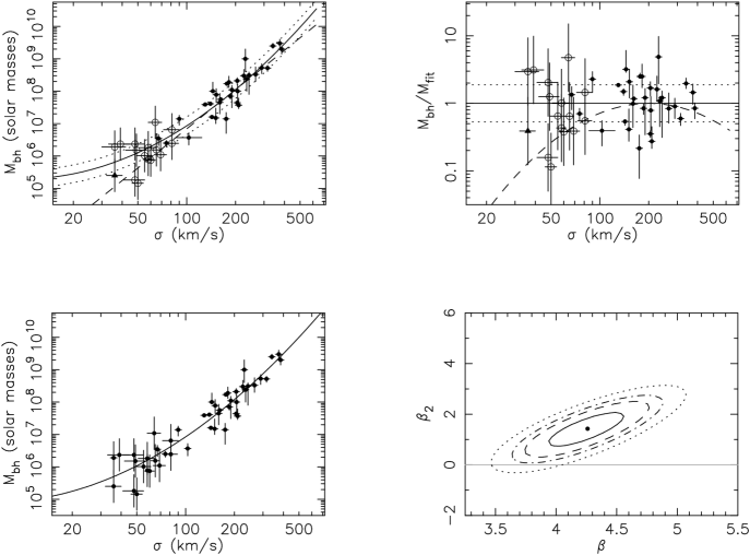
Figure 11: Upper Left: The best fit log-quadratic relation (determined from the Bayesian analysis of the Local sample) extrapolated to high and low $\sigma$ (solid line), and the level of intrinsic scatter around the best-fit relation (dotted lines). Also shown (dashed line) is the log-linear relation from T02. The points from the Local sample are shown (solid dots). In addition, the open circles represent SMBHs with masses estimated using AGN identified in SDSS (Barth, Greene & Ho. 2004). The triangle represents POX52 (Barth, Ho, Rutledge & Sargent 2004). Upper Right: The corresponding residuals relative to the log-quadratic relation, with dotted lines showing the best fit intrinsic scatter. The dashed line shows the additional residual of the log-quadratic relation relative to the log-linear relation. Lower Left: The combined sample of Local and AGN SMBHs with the resulting best-fit log-quadratic relation determined from a $\chi^{2}$ analysis. Lower Right: The resulting contours of $\chi^{2}$ (minimised over $\alpha$) of $\beta$ and $\beta_{2}$. Projections of the contours correspond to the 1, 1.5, 2 and 2.5-sigma limits on individual parameters. The point shows the most likely solution.

9.4 The low mass $M_{\rm bh}-\sigma$ relation

There are no SMBHs in the Local sample with masses below $\sim 2\times 10^{6}M_{\odot}$. Attempts to extend the $M_{\rm bh}-\sigma$ relation to lower masses through dynamical observations have centered on two cases, M33 (Merritt, Ferrarese & Joseph 2001; Gebhardt et al. 2001), and NGC205 (Valluri, Ferrarese, Merritt & Joseph 2005). Only upper limits have been obtained in these systems. However we can compare the log-quadratic fit in the low-$\sigma$ regime with SMBH masses obtained from single epoch virial estimates based on observations of AGN. The upper panel of figure 11 shows the extrapolation of the best fit log-quadratic relation for the Local sample, and its comparison to the AGN SMBH masses and velocity dispersions presented in Barth, Greene & Ho (2004), as well as the point for POX52 (Barth, Ho, Rutledge & Sargent 2004). The AGN SMBH masses in this sample were estimated using the single epoch virial mass calibration of Onken et al. (2004). The log-quadratic fit derived using the Local sample appears to describe the SMBH masses in these AGN much better than the log-linear fit (see right-hand panel of Figure 11). The residuals are symmetrically placed around the best fit log-quadratic relation. On the other hand the dashed line in the right hand panel of figure 11 shows the additional residual of the log-quadratic relation relative to the log-linear relation. The residuals of the AGN SMBHs relative to the log-linear relation are systematically positive, indicating that the log-linear relation provides a poor description.

The single epoch virial SMBH masses for the AGN have been estimated in a regime where the technique is not directly calibrated. One must therefore be cautious comparing the AGN and local samples since the AGN SMBH mass estimates may contain some unknown systematic uncertainty relative to the dynamical estimates of the Local sample (Barth, Greene & Ho 2005 did not perform a fit to the combined sample for this reason). Moreover it is possible that the AGN SMBH sample is biased towards large SMBH masses (Barth, Greene & Ho 2005). Never-the-less it is instructive to combine the Local and AGN SMBH samples and investigate the resulting log-quadratic $M_{\rm bh}-\sigma$ relation. We have repeated the $\chi^{2}$ minimisation using equation (4) for the combined sample of $N_{\rm g}=47$ SMBHs. In the lower-left panel of figure 11 we show the combined sample with the resulting best-fit $M_{\rm bh}-\sigma$ relation over-plotted (solid line). The intrinsic scatter required for a reduced $\chi^{2}$ of unity in this fit was $\epsilon_{\rm intrins}=0.22$ dex. In the lower-right panel of figure 11 we show the 1, 1.5, 2 and 2.5-sigma ellipsoids for $\beta$ and $\beta_{2}$. The most likely solution has $\beta=4.25$ and $\beta_{2}=1.3$ with 1-sigma uncertainties of 0.3 and 0.7 respectively. This solution is very close to the one obtained using only SMBHs in the Local sample ($\beta=4.3\pm 0.35$, $\beta_{2}=1.9\pm 1.1$ and $\epsilon_{\rm intrins}=0.25$ dex), indicating that the AGN SMBHs follow the same log-quadratic $M_{\rm bh}-\sigma$ relation as the Local sample. However the addition of low-mass AGN SMBHs results in a fit with a log-quadratic term which is non-zero at greater than the 2-sigma level. The sample of AGN SMBHs therefore support a log-quadratic $M_{\rm bh}-\sigma$ relation. The log-quadratic relation describes the masses of SMBHs in galaxies with velocity dispersions ranging from 25-400km s^-1. If one extrapolates this to lower $\sigma$ then the log-quadratic relation offers the tantalising prediction that there is a minimum SMBH mass of $\sim 10^{5}M_{\odot}$, and that this minimum SMBH mass resides in bulges with $\sigma\sim 10$km s^-1. Interestingly, this velocity dispersion corresponds to the minimum value of the virial velocity for a dark-matter halo within which gas accreted from the IGM can cool via atomic transitions in hydrogen.

9.5 The relation between $\beta$ and $\beta_{\rm bulge}$

Finally we would like to make the following point regarding the relationship between the power-law slope of the $M_{\rm bh}-\sigma$ and $M_{\rm bh}-M_{\rm bulge}$ relations. An estimate of the bulge mass may be made using the virial mass, $M_{\rm bulge}\sim M_{\rm bulge,vir}\propto\sigma^{2}R_{\rm e}$, where $R_{\rm e}$ is the scale radius of the bulge. The projection of the fundamental plane yields a relation between radius and velocity dispersion of $R_{\rm e}\propto\sigma^{1.5}$ (Bernardi et al. 2003). Consider the power-law slope at the mean velocity of the galaxy sample ($\sigma\sim 200$km/s). We have $M_{\rm bh}\propto(M_{\rm bulge})^{\beta_{\rm bulge}}$, which implies $M_{\rm bh}\propto\sigma^{3.5\beta_{\rm bulge}}$, or $\beta=3.5\beta_{\rm bulge}$. This is in excellent agreement with the best fit parameters of $\beta\sim 4.2$ and $\beta_{\rm bulge}=1.15$ derived in this paper. Furthermore, a value of $\beta=3.5$ for the $M_{\rm bh}-\sigma$ relation is ruled out at $\sim 80\%$ significance. If it is to be consistent with the $M_{\rm bh}-\sigma$ relation, the $M_{\rm bh}-M_{\rm bulge}$ relation should therefore be steeper than linear for galaxies with $\sigma\sim 200$km/s. Given the relation between $\sigma$ and the virial mass, we would also expect the $M_{\rm bh}-M_{\rm bulge}$ relation to have a positive quadratic component, given a positive quadratic component in the $M_{\rm bh}-\sigma$ relation.

10 Conclusion

Using the Local sample of SMBHs we have demonstrated that the parameter describing a log-linear fit to the $M_{\rm bh}-\sigma$ relation is sensitive to the inclusion of individual galaxies at a level larger than the statistical uncertainty. This indicates that a log-linear $M_{\rm bh}-\sigma$ relation does not provide a good description of the Local sample of SMBHs. We expand a general relation between $\log(M_{\rm bh})$ and $\log(\sigma/200\mbox{km}\,\mbox{s}^{-1})$ to second order, and fit the data using the resulting log-quadratic relation instead. We find that a log-quadratic relation provides a substantially better fit to the Local sample of SMBH masses and velocity dispersions. Moreover unlike the log-linear relation, the parameters describing the log-quadratic relation are not systematically dependent on the inclusion of individual galaxies in the sample.

After allowing for a second-order term in the $M_{\rm bh}-\sigma$ relation we find an unbiased estimate for the slope of the Local sample at $\sigma=200$km/s to be $\beta=4.2\pm 0.37$. This value is slightly (2/3-sigma) larger than previous estimates for this sample. However the logarithmic slope $d\log{M_{\rm bh}}/d\log{\sigma}$ of the best fit log-quadratic relation varies substantially, from 2.7-5.1 over the velocity range of the Local sample. The coefficient of the second order term $\beta_{2}=1.6\pm 1.3$ is greater than zero at the 90% level. This indicates that with 80% confidence the Local sample describes an $M_{\rm bh}-\sigma$ relation that does not follow a single powerlaw between $\sim 70$km/s and $\sim 380$km/s. We have tested the sensitivity of this conclusion to different sub-samples of SMBH masses determined via different techniques, as well as SMBHs with and without resolved spheres of influence. The log-quadratic fit implies a non-linear contribution to the $M_{\rm bh}-\sigma$ relation in a sub-sample of galaxies that contain only SMBHs whose spheres of influence were resolved, in a sub-sample containing only SMBHs with masses determined through stellar dynamics, and in a sub-sample containing only SMBHs with masses determined only by non stellar dynamical methods. Moreover the non-linearity is present in each sub-sample whether the central or effective velocity dispersion is used as the independent variable.

SMBH masses in active galaxies estimated via reverberation mapping offer an avenue to increase the SMBH sample for study of the $M_{\rm bh}-\sigma$ relation. We find that the combination of the 14 galaxies with reverberation SMBH masses and measured velocity dispersions (Onken et al. 2004) with the Local SMBH sample leads to a log-quadratic relation with the same best fit as the Local sample alone.

The $M_{\rm bh}-\sigma$ relation can be extended to lower masses through the inclusion of single epoch virial estimates of SMBH masses based on observations of AGN (Barth, Greene & Ho 2004). In a $\chi^{2}$ analysis the best-fit log-quadratic $M_{\rm bh}-\sigma$ relation is unchanged by the addition of a sample of 16 low mass SMBHs. However the uncertainty in $\beta_{2}$ is reduced. We find that in the absence of a systematic error in the normalisation of SMBH masses between the Local and AGN samples, the $M_{\rm bh}-\sigma$ relation described by the combined sample deviates from a power-law at greater than the 2-sigma level. The best-fit log-quadratic relation predicts a minimum mass for SMBHs in galaxies of $\sim 10^{5}M_{\odot}$, which should reside in bulges with $\sigma\sim 10$km s^-1.

A log-quadratic $M_{\rm bh}-\sigma$ relation has important implications for SMBH demography. In particular, estimates of the local SMBH mass-function that utilise the log-quadratic $M_{\rm bh}-\sigma$ relation describe densities of SMBHs with $M_{\rm bh}\ga 10^{9}M_{\odot}$ that are orders of magnitude larger than expected for a log-linear $M_{\rm bh}-\sigma$ relation. In addition the departure from a power-law should provide important clues regarding the astrophysics responsible for the $M_{\rm bh}-\sigma$ relation. For example one recent model describing the effects of radiative feedback on SMBH growth predicts departure from a power-law relation, including steepening of the relation at large $\sigma$ (Saznov et al. 2005).

We have also applied our analysis to the relation between SMBH and bulge mass using the sample described in Haering & Rix (2004). We find evidence for a log-quadratic term in the $M_{\rm bh}-M_{\rm bulge}$ relation (at the 1-sigma level), with $\beta_{\rm bulge}=1.15\pm 0.19$ and $\beta_{\rm 2,bulge}=0.12\pm 0.14$. We find an intrinsic scatter of $\delta_{\rm bulge}=0.41\pm 0.07$ dex. Since we find the intrinsic scatter in the $M_{\rm bh}-\sigma$ relation to be $\delta=0.28\pm 0.04$ dex, there is $\sim 50\%$ more scatter in the SMBH mass at fixed bulge mass than at fixed velocity dispersion.

The sample of kinematically detected SMBHs will not grow by a large factor in the foreseeable future (Ferrarese 2003). Progress in understanding the statistical properties of the SMBH population will instead come via estimates of SMBH masses that are based on reverberation mapping studies. The increased sample of SMBHs will offer the possibility of more clearly defining the local $M_{\rm bh}-\sigma$ relation (Gebhardt et al. 2000b; Ferrarese et al. 2001; Onken et al. 2004; Peterson et al. 2004; Nelson et al 2004), and of extending its study to high redshift (Shields et al. 2003).

Appendix A Comparison of parameters for different SMBH samples

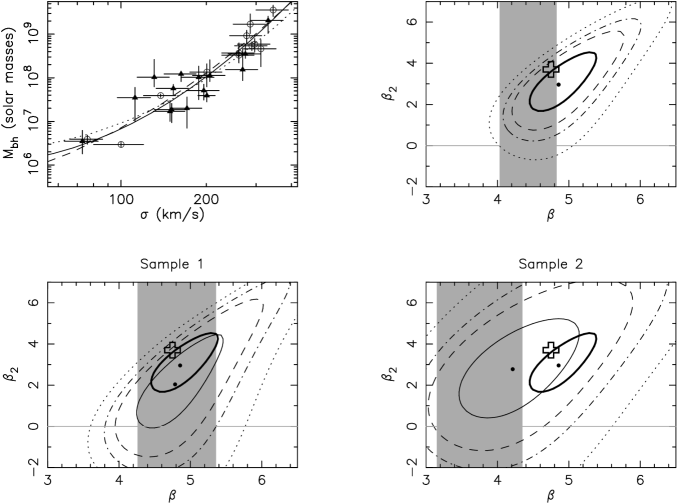
Figure 12: Log-quadratic fits to the samples of Ferrarese & Merritt (2000, sample 1), the additional galaxies added by Gebhardt et al. (2000, sample 2), as well as a combined sample (upper right panel) as described in Merritt & Ferrarese (2001). Projections of the contours represent the 1, 1.5, 2 and 2.5-sigma uncertainties on individual parameters. The 1-sigma error ellipse for the combined sample is repeated in the lower panels. In this figure the correlation is between SMBH mass and the central velocity dispersion (Ferrarese & Merritt 2000). The grey region shows the corresponding linear fit value for $\beta$ from Merritt & Ferrarese (2001). The upper left panel shows the three best fits along with the data. Sample-1 is represented by open circles, and sample-2 by triangles. The large cross shows the point $\beta=4.9$, $\beta_{2}=3.75$ which lies inside the 1-sigma error ellipses of all three samples in both the cases where central and effective velocity dispersion are used as the independent variable.

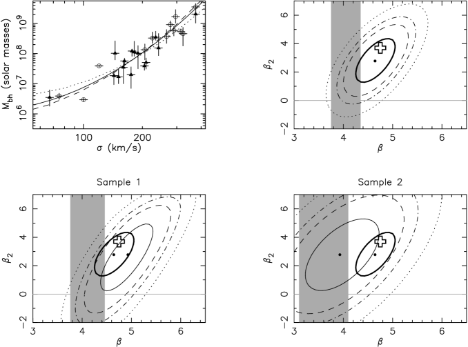
Figure 13: Log-quadratic fits to the samples of Ferrarese & Merritt (2000, sample 1), the additional galaxies added by Gebhardt et al. (2000, sample 2), as well as a combined sample (upper right panel) as described in Merritt & Ferrarese (2001). Projections of the contours represent the 1, 1.5, 2 and 2.5-sigma uncertainties on individual parameters. The 1-sigma error ellipse for the combined sample is repeated in the lower panels. In this figure the correlation is between SMBH mass and the effective velocity dispersion (Gebhardt et al. 2000). The grey region shows the corresponding linear fit value for $\beta$ from Merritt & Ferrarese (2001). The upper left panel shows the three best fits along with the data. Sample-1 is represented by open circles, and sample-2 by triangles. The large cross shows the point $\beta=4.9$, $\beta_{2}=3.75$ which lies inside the 1-sigma error ellipses of all three samples in both the cases where central and effective velocity dispersion are used as the independent variable.

Following the discovery of the $M_{\rm bh}-\sigma$ relation (Gebhardt et al. 2000, Ferrarese & Merritt 2000), there has been debate in the literature among the different groups regarding inconsistencies in the value of the measured slope. These differences have been attributed to several causes including use of biased statistics (Merritt & Ferrarese 2001) and systematic differences in the velocity dispersions used for the host galaxies (T02). We have shown that the slope $\beta$ of a log-linear relation is substantially changed by the presence or absence of one or a couple of the smallest galaxies in the sample. Given the different samples of velocity dispersions that have been employed by the different groups, the bias introduced by the assumption of a log-linear relation may therefore be more or less significant for different samples.

Merritt & Ferrarese (2001) presented an analysis of the log-linear relation for three different samples. The first two samples were drawn from Ferrarese & Merritt (2000, sample 1), and from the additional galaxies presented by Gebhardt et al. (2000, sample 2). The accuracy of some of the additional SMBH masses included by Gebhardt et al. (2000) has been called into question on the basis that the SMBH sphere of influence was not resolved (e.g. Merritt & Ferrarese 2001). In addition, Merritt & Ferrarese (2001) discuss the combined sample from these two sub-samples. For sample 2 Merritt & Ferrarese (2001) computed aperture corrected central velocity dispersions, so that all galaxies in the combined sample could be considered when estimating correlations between SMBH mass and both a central (Ferrarese & Merritt 2000) and an effective velocity dispersion (Gebhardt et al. 2000). Merritt & Ferrarese (2001) present fits for the slope $\beta$ of a log-linear relation to these samples using regression with bi-variate errors and intrinsic scatter (their label BRS).

We first consider the correlation of SMBH mass with central velocity dispersion (Ferrarese & Merritt 2000). Merritt & Ferrarese (2001) find $\beta=4.81\pm 0.55$ and $\beta=3.75\pm 0.59$ for samples 1 and 2 respectively. For the combined sample they get $\beta=4.43\pm 0.39$. Samples 1 and 2 differ at the 2-sigma level, while the combined sample leads to a slope that lies between the two. To mimic this analysis for a log-quadratic relation we minimise the following $\chi^{2}$ statistic

$$\chi^{2}=\sum_{i=1}^{N_{\rm g}}\frac{(y_{i}-\alpha-\beta x_{i}-\beta_{2}x_{i}^{2})^{2}}{\epsilon_{\rm intrins}^{2}+\epsilon_{yi}^{2}+(\beta^{2}+2\beta_{2}x_{i})^{2}\epsilon_{xi}^{2}},$$ (16)

where $y_{i}$ and $x_{i}$ are the logarithm of SMBH mass in solar masses and the logarithm of velocity dispersion in units of 200km/s respectively. The variables $\epsilon_{xi}$ and $\epsilon_{yi}$ are the uncertainties in dex for these parameters. The variable $\epsilon_{\rm intrins}$ is the intrinsic scatter, adjusted to yield a reduced $\chi^{2}$ of unity for the best-fit solution. In figure 12 we show the 1, 1.5, 2 and 2.5-sigma error ellipsoids for $\beta$ and $\beta_{2}$ in sample-1, sample-2 and the combined sample. The 1-sigma ellipsoid for the combined sample is shown in the other panels for comparison, and the best fit relations are plotted over the data in the upper left panel. The grey regions represent the 1-sigma range for $\beta$ determined by Merritt & Ferrarese (2001). The ellipsoids show that all three samples suggest a positive quadratic term is present in the $M_{\rm bh}-\sigma$ relation. The values of $\beta$ determined by Merritt & Ferrarese (2001) are conditional probabilities for $\beta$ given $\beta_{2}=0$, and so should correspond to regions where the error ellipsoids cross the $\beta_{2}=0$ line. Figures 12 and 13 show this to be the case. The inclusion of a quadratic term in the relation leads to similar estimates for parameters using each sample, with $\beta\sim 5$ and $\beta_{2}\sim 4$ lying inside the 1-sigma ellipsoids.

We also investigate the correlation between SMBH mass and effective velocity dispersion (Gebhardt et al. 2000). The values for effective velocity dispersion $\sigma$ in Gebhardt et al. (2000) did not include an estimate of the uncertainty. In the absence of quoted uncertainties, Merritt & Ferrarese (2001) assumed different values for the uncertainty in effective velocity dispersion and showed that increasing the uncertainty lead to steeper best fit slopes, and to consistency between fits for samples 1 and 2. T02 has since advocated 5% for the fractional uncertainty in effective velocity dispersion. We assume 5% errors in $\sigma$ and adopt $\sigma=100$km/s for the Milky-Way. In this case Merritt & Ferrarese (2000) found $\beta=3.6\pm 0.5$ and $\beta=4.11\pm 0.35$ for samples 1 and 2 respectively. For the combined sample, they found $\beta=4.05\pm 0.3$. In figure 13 we show the results for the log-quadratic fit in this case. The results are consistent for a log-quadratic relation, with $\beta\sim 4.6$ and $\beta_{2}\sim 3$ lying inside the 1-sigma error ellipses of all three samples. Consistency between the best fit log-quadratic relations for samples 1 and 2 therefore does not require uncertainties in $\sigma$ to be larger than 5%, the value advocated by the Nuker team (Gebhardt et al. 2003).

Finally we compare the estimates of $\beta$ and $\beta_{2}$ for relations between SMBH mass, and the central or effective velocity dispersions using the combined sample. The use of an effective velocity dispersion (with 5% uncertainty) leads to smaller values of $\beta$ and $\beta_{2}$ relative to a fit using central velocity dispersions. Merritt & Ferrarese (2001) found that this difference could be removed by increasing the uncertainty in $\sigma$ to greater than 10%. However a solution with $\beta\sim 4.9$ and $\beta_{2}\sim 3.5$ lies inside the 1-sigma error ellipsoids in both cases. Overall we find that a solution with $\beta\sim 4.75$ and $\beta_{2}\sim 3.7$ (shown by the large cross in figures 12 and 13) lies on or inside the 1-sigma error ellipsoids of all three samples using either the central or the effective velocity dispersions as the independent variable. Therefore if a log-quadratic $M_{\rm bh}-\sigma$ relation is used we find that there is no significant disparity between the different samples.

Appendix B An updated sample of SMBH mass and central velocity dispersion

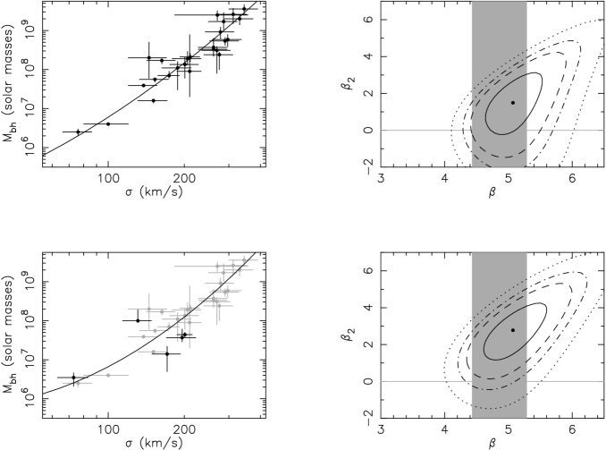
Figure 14: Upper left: The sample of 25 SMBHs with reliable masses and resolved spheres of influence described in Ferrarese & Ford (2004). Upper right: The resulting contours of $\chi^{2}$ (minimised over $\alpha$) of $\beta$ and $\beta_{2}$. Projections of the contours correspond to the 1, 1.5, 2 and 2.5-sigma limits on individual parameters. The point shows the most likely solution. Lower left and right: As for the upper row, but including the additional 5 SMBH masses in table II of Ferrarese & Ford (2004) classed as reliable but with unresolved spheres of influence (shown as dark points). The grey regions show the allowed range of $\beta=4.86\pm 0.43$ in a log-linear fit to the 25 SMBHs with a resolved sphere of influence (Ferrarese & Ford 2004).

In a recent review, Ferrarese & Ford (2004) have compiled an updated sample of local SMBHs, listed in their table-II. Of the 38 mass estimates, they class 8 as unreliable. Of the remaining 30 SMBHs, the mass observations resolved the sphere of influence in only 25 cases. Ferrarese & Ford (2004) used this sample of 25 reliable mass estimates where the sphere of influence is resolved to generate a log-linear fit to the $M_{\rm bh}-\sigma$ relation. They find a log-linear slope of $\beta=4.86\pm 0.43$. We have performed log-quadratic fits to this updated sample, and show the results in Figure 14. In the upper left panel we show the sample of 25 SMBHs with resolved spheres of influence, and the corresponding best-fit relation. In the upper right-hand panel we show the 1, 1.5, 2 and 2.5-sigma error ellipsoids of $\beta$ and $\beta_{2}$ for this sample. This sample prefers a log-quadratic relation, with the log-linear relation lying near the $\Delta\chi^{2}=1$ contour. The grey regions in Figure 14 represent the 1-sigma range for $\beta$ determined by Ferrarese & Ford (2004). We see that the contours of $\chi^{2}$ intercept the $\beta_{2}=0$ line over a range of slope described by the log-linear solution.

Of the 5 galaxies with reliable mass-estimates, but unresolved spheres of influence in Table II of Ferrarese & Ford (2004), 4 have had their stellar kinematical data modeled using both high-resolution spaced based data, and lower resolution ground based data (Gebhardt et al. 2003). Gebhardt et al. (2003) found that while higher resolution imaging led to a more precise determination, there was no systematic trend of the best fit values. We therefore repeat the above analysis with the inclusion of the 5 galaxies and show the results in the lower row of Figure 14. The additional 5 galaxies only change the slope $\beta$ of a log-linear fit by a small amount (significantly less than the error bar). Moreover, these 5 SMBH masses are evenly spread about the best-fit relation, indicating that there is no systematic bias due to their spheres of influence not being resolved. However the inclusion of these galaxies significantly increases the significance of a log-quadratic term in the $M_{\rm bh}-\sigma$ relation.

References

- [Aller & Richstone(2002)] Aller, M. C., & Richstone, D. 2002, Astron. J., 124, 3035
- [Bacon et al.(2001)] Bacon, R., Emsellem, E., Combes, F., Copin, Y., Monnet, G., & Martin, P. 2001, Astron. Astrophys., 371, 409
- [Barth et al.(2001)] Barth, A. J., Sarzi, M., Rix, H., Ho, L. C., Filippenko, A. V., & Sargent, W. L. W. 2001, ApJ., 555, 685
- [Barth et al.(2004)] Barth, A. J., Ho, L. C., Rutledge, R. E., & Sargent, W. L. W. 2004, ApJ., 607, 90
- [Barth et al.(2005)] Barth, A. J., Greene, J. E., & Ho, L. C. 2005, ApJ. Lett., 619, L151
- [Bower et al.(2001)] Bower, G. A., et al. 2001, ApJ., 550, 75
- [Bernardi et al.(2003)] Bernardi, M., et al. 2003, Astron. J., 125, 1866
- [Cappellari et al.(2002)] Cappellari, M., Verolme, E. K., van der Marel, R. P., Kleijn, G. A. V., Illingworth, G. D., Franx, M., Carollo, C. M., & de Zeeuw, P. T. 2002, ApJ., 578, 787
- [Cretton & van den Bosch(1999)] Cretton, N., & van den Bosch, F. C. 1999, ApJ., 514, 704
- [Ferrarese et al.(1996)] Ferrarese, L., Ford, H. C., & Jaffe, W. 1996, ApJ., 470, 444
- [Ferrarese & Ford(1999)] Ferrarese, L., & Ford, H. C. 1999, ApJ., 515, 583
- [Ferrarese & Merritt(2000)] Ferrarese, L., & Merritt, D. 2000, ApJ. Lett., 539, L9
- [Ferrarese et al.(2001)] Ferrarese, L., Pogge, R. W., Peterson, B. M., Merritt, D., Wandel, A., & Joseph, C. L. 2001, ApJ. Lett., 555, L79
- [Ferrarese(2002)] Ferrarese, L. 2002, Current high-energy emission around black holes, 3
- [Ferrarese(2003)] Ferrarese, L. 2003, Astronomical Society of the Pacific Conference Series, 291, 196
- [Ford et al.(1994)] Ford, H. C., et al. 1994, ApJ. Lett., 435, L27
- [Gebhardt et al.(2000)] Gebhardt, K., et al. 2000, ApJ. Lett., 539, L13
- [Gebhardt et al.(2000b)] Gebhardt, K., et al. 2000, ApJ. Lett., 543, L5
- [Gebhardt et al.(2003)] Gebhardt, K., et al. 2003, ApJ. Lett., 583, 92
- [Gebhardt et al.(2003)] Gebhardt, K., et al. 2001, ApJ., 583, 92
- [Graham et al.(2002)] Graham, A. W., Erwin, P., Caon, N., & Trujillo, I. 2002, Astronomical Society of the Pacific Conference Series, 275, 87
- [Greenhill & Gwinn(1997)] Greenhill, L. J., & Gwinn, C. R. 1997, Astrophys. Sp. Sc., 248, 261
- [Häring & Rix(2004)] Häring, N., & Rix, H. 2004, ApJ. Lett., 604, L89
- [Harms et al.(1994)] Harms, R. J., et al. 1994, ApJL, 435, L35
- [Herrnstein et al.(1999)] Herrnstein, J. R., et al. 1999, Nature, 400, 539
- [Huchra et al.(1990)] Huchra, J. P., Geller, M. J., de Lapparent, V., & Corwin, H. G. 1990, ApJ. Supp., 72, 433
- [King(2003)] King, A. 2003, ApJ. Lett., 596, L27
- [Kormendy et al.(1998)] Kormendy, J., Bender, R., Evans, A. S., & Richstone, D. 1998, Astron. J., 115, 1823
- [Kormendy & Bender(1999)] Kormendy, J., & Bender, R. 1999, ApJ., 522, 772
- [Kormendy & Richstone(1995)] Kormendy, J., & Richstone, D. 1995, Ann. Rev. Astron. Astrophys., 33, 581
- [Kormendy et al.(1996)] Kormendy, J., et al. 1996, ApJ. Lett., 459, L57
- [Macchetto et al.(1997)] Macchetto, F., Marconi, A., Axon, D. J., Capetti, A., Sparks, W., & Crane, P. 1997, ApJ., 489, 579
- [Magorrian et al.(1998)] Magorrian, J., et al. 1998, Astron. J., 115, 2285
- [Marconi & Hunt(2003)] Marconi, A., & Hunt, L. K. 2003, ApJL, 589, L21