Constraints on Topological Defects Energy Density from First-Year WMAP Results

Abstract

We compare the predictions of hybrid inflationary models that produce both adiabatic fluctuations and topological defects to first year WMAP results. We use a Markov Chain Monte Carlo method to constrain the contribution of cosmic strings and textures to the CMB angular power spectrum. Marginalizing this contribution over the cosmological parameters of a power law flat $\Lambda$CDM model, we place a 95% upper limit of 23% on the topological defects contribution to density fluctuations, the maximum likelihood being of order 4%. This corresponds to an upper limit on the string scale of $G\mu\leq 3.2\times 10^{-7}$. We also explore the degeneracies between the defects contribution and other cosmological parameters.

I.  INTRODUCTION

In the 1980’s and 1990’s, cosmologists focused on two plausible scenarios, each of which produces scale invariant density fluctuations. In the inflationary model, quantum fluctuations are amplified during inflation and produce adiabatic, gaussian and nearly scale invariant fluctuations Linde . This model is successful in resolving some issues of the Hot Big Bang Model Dodelson and is in good agreement with observations over a wide range of scales WMAPbestfit .

The alternative defects scenario rests on the realization that since the Universe has steadily cooled down since the Planck time, spontaneous breaking of symmetries must have occurred. Each symmetry breaking may lead to the creation of topological defects such as monopoles, textures, domain walls, or cosmic strings Vilenkin . A non negligible contribution of monopoles and domain walls is ruled out by some basic observations Srivastava . However, textures, which appear when a non-Abelian symmetry is spontaneously and completely broken, and cosmic strings, due to a $U(1)$ symmetry breaking phase transition, are both liable. Even if they are not the dominant source of fluctuations, they may still make detectable contributions to the CMB and large scale structures formation.

Hybrid inflationary models, e.g., D- and F-term inflationary models, predict that there should be both quantum fluctuations, occurring during the inflationary phase, and topological defects, created at the end of inflation Kibble , which also induce anisotropies in the CMB by gravitational effects Kolb .

Some recent papers Dterm on these models conclude that cosmic strings should be responsible for at least 50%, and at most 85%, of the amplitude of fluctuations in the CMB anisotropies power spectrum. However, other works Rocher give a much smaller contribution of cosmic strings for the same models, and the contribution of topological defects is highly constrained Bouchet (best fit with a 18% contribution) from measurements previous to WMAP, in favor of adiabatic fluctuations.

In this Letter, we study the constraints coming from first year WMAP results. WMAP has indeed given unprecedented precise results on fluctuations in the CMB. It is therefore worth studying how models involving topological defects can fit its data, and what are the foldings of the constraints hereby established on existing inflationary models, previous constraints, and cosmological parameters.

II.  MODEL AND METHOD

As a non negligible contribution of monopoles and domain walls is ruled out, we only consider cosmic strings (CS) and textures (TX) in this work and we assume a model, in which the power spectrum of the CMB anisotropies is written:

$$C_{\ell}^{model}=\left(1-\beta-\gamma\right)\,C_{\ell}^{AD}+\beta\,C_{\ell}^{CS}+\gamma\,C_{\ell}^{TX}$$ (1)

where $\left(\beta,\gamma\right)\in\left[0;1\right]^{2}$, $\beta+\gamma\leq 1$ and $AD$ stands for adiabatic. The theoretical power spectra of temperature, and electric type polarization for strings and textures have already been computed by Seljak, Pen & Turok seljak . Many tests seljaktest have been performed on the procedure leading to these results, and other independent works allen have given similar conclusions, all of them being consistent to within about 10%. These results suggest that, for $\ell\leq 1000$, the amplitude of fluctuations in the power spectra of electric type polarization and magnetic type polarization for cosmic strings and textures, can be safely neglected compared to the one in the power spectrum of temperature. Moreover, the predicted power spectra for cosmic strings and textures are so close for these values of $\ell$ that it is reasonable to consider that they are the same. Thus, we assume that $C_{\ell}^{CS}$ and $C_{\ell}^{TX}$ are the one shown on Fig. 1, and we can simplify equation (1) to

$$C_{\ell}^{model}=\left(1-\alpha\right)\,C_{\ell}^{AD}+\alpha\,C_{\ell}^{TD}$$ (2)

where $C_{\ell}^{TD}$ can be $C_{\ell}^{CS}$ as well as $C_{\ell}^{TX}$, and $0\!\leq\!\alpha\nobreak\leq\nobreak 1$ is the contribution of topological defects to the CMB anisotropies power spectrum.

To generate the adiabatic spectrum, we use CMBwarp cmbwarp , a fast CMB code that agrees well with the more accurate CMBFast results. In the parameter range of interest, the largest differences between these two codes are generally less than 1%. For the calculations in this paper, we assume a simple power law flat $\Lambda$CDM model. We choose to normalize both $C_{\ell}^{AD}$ and $C_{\ell}^{TD}$ so that, whatever the values of $\alpha$, the matter power spectrum normalization is the one corresponding to WMAP best fit as computed by CMBwarp with WMAP best fit cosmological parameters WMAPbestfit .

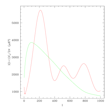
Figure 1: CMB angular power spectrum induced by cosmic strings and textures alone (green) and by a simple power law flat $\Lambda$CDM model corresponding to WMAP best fit (red). We normalize these spectra so that the matter power spectrum normalization for our model is the same as WMAP best fit for a flat $\Lambda$CDM model without topological defects. It should be noticed that the points of the green plot have not been recomputed but directly extracted from the study of Seljak, Pen and Turok seljak .

Thus, our model is chosen as a flat $\Lambda$CDM model to which we add the contribution of topological defects, so that it can be described with only 7 parameters: the baryon density ($\omega_{b}$), the matter density ($\omega_{m}$), Hubble constant ($h$), the perturbation normalization ($A$), the optical depth ($\tau$), the spectral index ($n_{s}$), and the contribution of topological defects to the power spectrum ($\alpha$). The idea is to estimate the values of each of these seven parameters with 1- 2- and 3-$\sigma$ confidence contours in the 7-D parameter space.

To investigate the likelihood space, we use a Markov Chain Monte Carlo (MCMC) method christensen , which enables us to evaluate the likelihood of $\sim 5\times 10^{5}$ models in approximatively 7 hours. This method is based on Bayes’ theorem, which states that the probability to have the set of parameters $s$ given the observed $\mathcal{C}_{\ell}$ is

$$\mathcal{P}(s|\mathcal{C}_{\ell})=\frac{\mathcal{P}(\mathcal{C}_{\ell}|s)\,\mathcal{P}(s)}{\int{\mathcal{P}(\mathcal{C}_{\ell}|s)\,\mathcal{P}(s)\,ds}}$$ (3)

where $\mathcal{P}(\mathcal{C}_{\ell}|s)$ is the likelihood of observing $\mathcal{C}_{\ell}$ given the set of parameters $s$, and $\mathcal{P}(s)$ the prior probability density. This theorem tells us we can figure out the value of $\mathcal{P}(s|\mathcal{C}_{\ell})$, what we would like to do, from the likelihood of obtaining the observed $\mathcal{C}_{\ell}$ from our set of parameters $s$, that we can compute with the likelihood code provided by the NASA/WMAP Science Team on LAMBDA, provided we specify priors. Postulating the equidistribution of ignorance, we assume that each cosmological parameter has the same probability to have each value between the following lower and upper bounds:

$\begin{array}[]{cc}0\leq\omega_{b}\leq 1&0\leq\omega_{m}\leq 1\\ 0.5\leq h\leq 1.5&0.5\leq A\leq 2.5\\ 0\leq\tau\leq 0.3&0\leq n_{s}\leq 2\end{array}$

It should be noticed, as we will see later, that these priors have no effect on our results, as the MCMC never encounters the priors’ boundaries, at the exception of $\tau$. For this latter, the prior enables the MCMC not to enter unphysical regions of the parameter space.

Given these priors and Bayes’ theorem, we can then explore the likelihood surface by computing the likelihood of the model obtained after each step, until we find the most likely region for our cosmological parameters to be. We use the algorithm of Verde for this exploration, and the chain is stopped when we can make sure it has properly converged (we will study this criterion in details as a check of our results), which means we have reached and stayed long enough in the region of the parameters space of highest likelihood, and that the parameter space has been widely explored.

In this work, we consider the situations in which the TT and TE components of the power spectrum are affected by topological defects. Considering the TT data only, or the TT and TE components of the power spectrum, does not change the results, among which is Fig. 2.

III.  RESULTS AND DISCUSSION

These results show that $\alpha$ is more likely to be found between 0.02 and 0.15 at 1-$\sigma$ with a maximum likelihood around 0.04, but scenarios involving a zero contribution of topological defects are authorized at 2-$\sigma$. It is to be noticed that our priors let $\alpha$ free to take any values. Nevertheless, we see that a contribution of more than 29% is completely excluded at 3-$\sigma$. Moreover, we find three main degeneracies between our parameters: when the value of $\alpha$ increases, so do the values of $\omega_{b}$, $n_{s}$ and $h$. Each of these parameters increases linearly with $\alpha$.

This can be easily understand by looking at the respective shapes of $\mathcal{C}_{\ell}^{TD}$ and $\mathcal{C}_{\ell}^{AD}$ WMAPbestfit . Indeed, the spectrum induced by topological defects gives a very low contribution to the second peak. Therefore, if we keep the cosmological parameters constant and $\alpha$ increases, which means that the adiabatic contribution goes down, the height of the second peak will diminished, so that it will become incompatible with WMAP results. As our program looks for the most likely set of cosmological parameters compatible with WMAP, it has to modify the values of the cosmological parameters, in a way that this discrepancy is canceled. In other words, the cosmological parameters should be modified in a way that the height of the second peak increases whereas the one of the first peak does not change significantly. That is done by decreasing $\Omega_{b}$ (which makes the first peak decreases and the second peak increases) and increasing $h$ (which makes the first and second peak increases). We can check this behavior of $h$ directly on Fig. 2. To verify that the evolution of $\Omega_{b}$ is the one predicted, we have to consider the graph giving $\omega_{b}$, where we can see that $\omega_{b}$ increases with $\alpha$, but less than $h^{2}$ does, which confirm the decrease of $\Omega_{b}$.

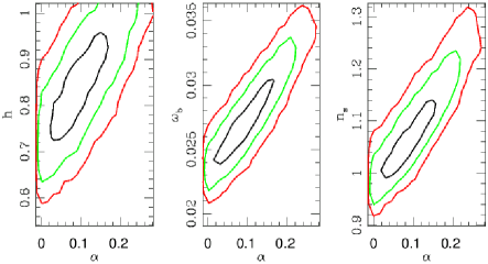
Figure 2: We plot the 1-$\sigma$ (black), 2-$\sigma$ (green) and 3-$\sigma$ (red) confidence contours for first year WMAP data for three parameters: $h$, $\omega_{b}$ and $n_{s}$. This indicates that scenarios involving a contribution of topological defects to the amplitude of fluctuations in the CMB greater than 29% are rejected at 3-$\sigma$, whereas a zero-contribution is possible at 2-$\sigma$. The 1-$\sigma$ contour implies a contribution between 2% and 15%, with a maximum likelihood of 4%. Each parameter on this graph is degenerated with $\alpha$.

Another degeneracy is the one between $\alpha$ and $n_{s}$: if $\alpha$ increases, so does $n_{s}$. Indeed when $\alpha$ increases, we replace a part of the contribution of the adiabatic spectrum by a contribution of topological defects. But, at large scales, $P(k)$ due to topological defects is more concave than $P(k)$ predicted by the adiabatic model, which can be taken as $P(k)\propto{k}^{n_{s}-1}$ Kolb with $n_{s}=0.99\pm 0.04$ WMAPbestfit . Thus, if we increase the contribution of topological defects, we must increase the convexity of the adiabatic spectrum to keep a shape compatible with WMAP results, that is to say that $n_{s}$ has to increase, which it does.

If we use the set of parameters corresponding to the maximum likelihood to compute the power spectrum, we find a spectrum in excellent agreement with WMAP best fit: the first two peaks coincide perfectly. Nevertheless, a small discrepancy can be seen for the third peak. This is consistent with the model of the power spectrum induced by topological defects which gives a quasi-zero contribution after the second peak. Therefore, if the contribution of the adiabatic spectrum decreases, it is not compensated by the added contribution of topological defects, which makes the third peak decrease. Despite this feature, the fit is still compatible with WMAP results. It should also be noticed that this is true for each value of $\alpha$ included in the 1-$\sigma$ and 2-$\sigma$ contours; small discrepancies begin to appear in the 3-$\sigma$ area.

During this work, we became aware of the paper Pogosian , which uses a Bayesian analysis in a three dimensional parameter space to constrain the contribution of cosmic strings with first year WMAP data. In their work, $\omega_{m}$, $\omega_{b}$, $h$ and $\tau$ are chosen to be WMAP best fit values, and they study the likelihood of their model involving cosmic strings in a 3-D parameters space, the only non-topological parameter involved in this space being $n_{s}$. The results they find with this method are similar to ours concerning the best fit, but quite different as far as contours are concerned, and this can be easily explained. Indeed, in Pogosian almost all cosmological parameters are kept constant, at the exception of $n_{s}$, with their values corresponding to WMAP best fit, which the authors claim is allowed by the fact that the contribution of topological defects should be relatively small compared to the one of quantum fluctuations. This is absolutely true for the best fit which gives a contribution of cosmological defects of order $4\%$, the other cosmological parameters being very close to those estimated by the NASA/WMAP Science Team, as we have shown in this Letter. Nevertheless, this statement is wrong generally speaking. Indeed, we have seen that letting all parameters free to vary in the parameter space, shows strong degeneracies between some cosmological parameters (namely $h$, $\omega_{b}$, $n_{s}$ and $\alpha$) so that it is not possible to choose a parameter independently from the others. Doing so necessarily leads to wrong estimations of contours, which explain the differences between our results and those given in Pogosian .

As we were ready to submit this Letter, wyman , in which a work similar to ours is conducted, was posted and gives results consistent with our work. However, in this paper, the authors use the power spectrum induced by local cosmic strings, instead of the global strings we consider. Its shape corresponds to the one we display on Fig. 1, but the peak that is located around $\ell\sim 150$ on our power spectrum is to be found at $\ell\sim 450$ in wyman . The interesting point is that, even with this difference, we still get similar results. This suggests that the results obtained by the method we both use is qualitatively insensitive to the model of cosmic strings we consider.

There are two main risks when using a MCMC. First of all, we have to make sure that the chain converges properly, that is to say that we have reached a situation in which the likelihood oscillates with a small amplitude around a mean value which will be the center of the most likely region for the cosmological parameters to be. Moreover, as the chain is necessarily finished, we cannot have access to all areas of the 7-D parameter space. But we have to be sure that we sufficiently explore this space, in other words, that we do not forget the exploration of entire areas of the parameter space.

To check these two aspects, we use the approach described in Verde and use the method of gelman , which states that the MCMC gives reliable results if the quantity

$$R=\left(1-\frac{1}{n_{e}}\right)+\frac{B}{W}\,\left(1+\frac{1}{n_{c}}\right)$$ (4)

where $W$ is the within-chain variance and $B$ the between-chain variance, is smaller than 1.2 when computed on $n_{c}$ chains each of which contains $2n_{e}$ elements, from which we consider only the last $n_{e}$. In this work, we are more conservative and we have chosen to require $R\sim 1.1$. This result is obtained with 10 chains of 100,000 steps. We also discard the first 5,000 points of each chain, to eliminate the so-called burn-in zone, during which the stationary distribution might not be reached. The results are absolutely not sensitive to this last choice, which is an additional clue showing that we consider enough points in the stationary distribution.

V.  CONCLUSION

The first year data of WMAP enable to reject at $3\mbox{-}\sigma$ scenarios involving a contribution of more than 29% of topological defects, and so, in particular, of cosmic strings. In other words, D- and F-term inflationary models involving a contribution of more than 50% Dterm do not match WMAP data, and so, cannot be acceptable scenarios. But most D- and F-term inflationary models predict more reasonable contributions of defects. For example, Urrestilla, Achúcarro & Davis Dwithoutcs present a superstring-inspired D-term inflation scenario which does not lead to the formation of cosmic strings. Another example is Rocher & Sakellariadou Rocher who show that in the context of global supersymmetry, for F-term inflation, and local supersymmetry, for D-term inflation, these models can lead to contributions compatible with our study.

We have also shown in this Letter that we cannot reject models involving a low contribution (between 2% and 15%) of topological defects, the best fit of WMAP data being given by a 4% contribution of topological defects, which gives a result as acceptable as a simple $\Lambda$CDM model. Concerning this point, this work goes in the same way as the results obtained by Bouchet et al. Bouchet with BOOMERanG data, despite the fact that our best fit gives a much smaller contribution for cosmic strings thanks to the precision of WMAP measurements.

Thus, looking at large scales is not sufficient to rule out or confirm models involving topological defects for the moment. But as WMAP will soon get more precise measurements of the CMB anisotropies for the third peak, it will be possible to increase the constraints on $\alpha$. It should also be worth looking at what topological defects imply at small scales. Experimental data usable for these scales will indeed soon be provided by some space or ground based experiments such as Planck or ACT, so that we will be able to compare theoretical predictions with observations.

- (1) A. Linde, Particle Physics and Inflationary Cosmology, (Harwood Academic, New York, 1990).
- (2) S. Dodelson, Modern Cosmology (Academic Press, 2003).
- (3) D. N. Spergel et al., Astrophys. J. Suppl. 148, 175 (2003).
- (4) A. Vilenkin and E. P. S. Shellard, Cosmic Strings and Other Topological Defects (Cambridge University Press, 1994).
- (5) A. M. Srivastava, Pramana-J. Phys. 53, 1069 (1999).
- (6) T. W. B. Kibble, Phys. Rept. 67, 183 (1980).
- (7) E. W. Kolb and M. S. Turner, The Early Universe (Westview Press, 1994).
- (8) R. Kallosh and A. Linde, JCAP 0310, 008 (2003); R. Jeannerot, Phys. Rev. D 56, 6205 (1997).
- (9) J. Rocher and M. Sakellariadou, hep-ph/0406120.
- (10) F. R. Bouchet, P. Peter, A. Riazuelo, and M. Sakellariadou, Phys. Rev. D. 65, 021301 (2001).
- (11) U. Seljak, U.-L. Pen, and N. Turok, Phys. Rev. Lett. 79, 1615 (1997).
- (12) N. Turok, U.-L. Pen, and U. Seljak, Phys. Rev. D. 58, 023506 (1997).
- (13) B. Allen et al., Phys. Rev. Lett. 79, 2624 (1997).
- (14) R. Jimenez, L. Verde, H. V. Peiris, and A. Kosowsky, Phys. Rev. D 70, 023005 (2004).
- (15) N. Christensen and R. Meyer, astro-ph/0006401
- (16) L. Verde et al., Astrophys. J. Suppl. 148, 195 (2003).
- (17) L. Pogosian, M. Wyman and I. Wasserman, JCAP 09, 008 (2004).
- (18) M. Wyman, L. Pogosian and I. Wasserman, astro-ph/0503364.
- (19) A. Gelman and D. Rubin, Stat. Sci. 7, 457 (1992).
- (20) J. Urrestilla, A. Achúcarro and A. C. Davis, Phys. Rev. Lett. 92, 251302 (2004).