Structural Parameters of the Hot Pulsating B Subdwarf PG~1219+534 from Asteroseismology^,

Over the last several years, we have embarked on a long term effort to exploit the strong potential that hot B subdwarf (sdB) pulsators have to offer in terms of asteroseismology. This effort is multifaceted as it involves, on the observational front, the acquisition of high sensitivity photometric data supplemented by accurate spectroscopic measurements, and, on the theoretical and modeling fronts, the development of appropriate numerical tools dedicated to the asteroseismological interpretation of the seismic observations. In this paper, we report on the observations and thorough analysis of the rapidly pulsating sdB star (or EC14026 star) PG~1219+534. Our model atmosphere analysis of the time averaged optical spectrum of PG~1219+534 obtained at the new Multiple Mirror Telescope (MMT) leads to estimates of $T_{{\rm{\rm eff}}}=$ 33,600 $\pm$ 370 K and $\log g=5.810\pm 0.046$ (with $\log N({\rm He})/N({\rm H})=-1.49\pm 0.08$), in good agreement with previous spectroscopic measurements of its atmospheric parameters. This places PG~1219+534 right in the middle of the EC14026 instability region in the $\log g-T_{{\rm eff}}$ plane. A standard Fourier analysis of our high signal-to-noise ratio Canada-France-Hawaii Telescope (CFHT) light curves reveals the presence of nine distinct harmonic oscillations with periods in the range $122-172$ s, a significant improvement over the original detection of only four periods by Koen et al. (1999). On this basis, we have carried out a detailed asteroseismic analysis of PG~1219+534 using the well-known forward method and assuming that the observed modes have $\ell\leq 3$. Our analysis leads objectively to the identification of the ($k$, $\ell$) indices of the nine periods observed in the star PG~1219+534, and to the determination of its structural parameters. The periods all correspond to low-order acoustic modes with adjacent values of $k$ and with $\ell=0$, 1, 2, and 3. They define a band of unstable modes, in close agreement with nonadiabatic pulsation theory. Furthermore, the average dispersion between the nine observed periods and the periods of the corresponding nine theoretical modes of the optimal model is only $\sim 0.6$%, comparable to the results of a similar analysis carried out by Brassard et al. (2001) on the rapid sdB pulsator PG 0014+067. On the basis of our combined spectroscopic and asteroseismic analysis, the inferred global structural parameters of PG~1219+534 are $T_{{\rm eff}}=$ 33,600 $\pm$ 370 K, $\log g=5.8071\pm 0.0057$, $\log M_{{\rm env}}/M_{*}=-4.254\pm 0.147$, $M_{*}=0.457\pm 0.012$ $M_{\odot}$, $R/R_{\odot}=0.1397\pm 0.0028$, and $L/L_{\odot}=22.01\pm 1.85$. Combined with detailed model atmosphere calculations, we estimate, in addition, that this star has an absolute visual magnitude $M_{V}=4.62\pm 0.06$ and is located at a distance $d=531\pm 23$ pc (using $V=13.24\pm 0.20$). Finally, if we interpret the absence of fine structure (frequency multiplets) as indicative of a slow rotation rate of that star, we further find that PG~1219+534 rotates with a period longer than $3.4$ days, and has a maximum rotational broadening velocity of $V\sin i\lesssim 2.1$ km.s^-1.

1 Introduction

Hot subdwarf B (sdB) stars are commonly interpreted as low-mass ($\sim 0.5$ $M_{\odot}$) core helium burning objects that belong to the so-called Extreme Horizontal Branch (EHB). Having extremely thin and mostly inert hydrogen rich residual envelopes ($M_{\rm env}<0.02$ $M_{\odot}$), these stars remain hot ($T_{\rm eff}\sim$ 22,000 – 42,000 K) and compact ($\log g\sim 5.2-6.2$) throughout their entire EHB lifetime and eventually evolve toward the white dwarf cooling sequence without experiencing the Asymptotic Giant Branch (AGB) and Planetary Nebulae (PN) phases of stellar evolution (see Dorman et al., 1993). If the fate of sdB stars is relatively well understood, their origin – i.e., how they form – is still unclear, however. The main difficulty resides in identifying how sdB stars manage to remove all but a very small fraction of their envelope at exactly the same time that they reach a sufficient core mass for helium flash ignition at the tip of the Red Giant Branch (RGB). Various formation scenarios have been proposed over the years to solve this problem, involving either single star evolution with enhanced mass loss at the tip of the RGB (D’Cruz et al., 1996), or binary evolution including various concurrent channels from common envelope ejection, stable Roche lobe overflow, to the merger of two helium white dwarfs (see, e.g., Han et al. 2002, 2003 and references therein). Interestingly, these authors suggest that the latter binary evolution scenarios would lead to a somewhat broader dispersion of stellar masses among sdB stars (between 0.30 – 0.70 $M_{\odot}$) than is currently assumed from canonical EHB models.

Renewed interest in this phase of stellar evolution has come in part from the recent discoveries of two new classes of multiperiodic nonradial pulsators among sdB stars which enable, in principle, the asteroseismic probe of their internal structure. The rapid sdB pulsators known as the V361 Hya stars, but more commonly referred to as the EC14026 stars, were the first to be observationally detected by colleagues from the South African Astronomical Observatory (SAAO; Kilkenny et al., 1997). Interestingly, at the same epoch, their existence was also independently predicted from theoretical considerations based on the identification of an efficient driving mechanism for the pulsations (Charpinet et al., 1996). The mechanism uncovered is a $\kappa$-effect due to local overabundances of heavy metals – especially of iron – produced by microscopic diffusion processes which are at work in the envelope of these stars (Charpinet et al., 1997). Various surveys by the SAAO group, by the Montréal group (see Billères et al., 2002), by a Norwegian-German-Italian team (see, e.g., Silvotti et al., 2002), and by other teams (see the reviews of Charpinet, 2001 and Kilkenny, 2002) rapidly led to additional discoveries, bringing the total of known EC14026 pulsators to 33 at the time of this writing. The EC14026 stars tend to cluster at high effective temperatures and surface gravities (near $T_{\rm eff}\sim$ 33,500 K and $\log g\sim 5.8$), although outliers indicate a relatively large dispersion of these stars in the $\log g-T_{\rm eff}$ plane. The periods detected in EC14026 stars typically range from $\sim 100$ s to $\sim 200$ s, but can be substantially longer for class members having lower surface gravities (e.g., 290–600 s for PG 1605+072; see Charpinet, 2001 and references therein). Their mode amplitudes usually span a relatively wide range, but typical values are of several millimagnitudes. In most cases, the short periods are entirely consistent with low-order, low-degree radial and nonradial acoustic waves (Stobie et al., 1997; Charpinet et al. 1997, 2001). However, in low surface gravity sdB pulsators, the presence in the observed period spectrum of low-order $g$-modes or mixed modes having both $p$- and $g$-mode properties cannot be excluded and somewhat complicates the identification of the true nature of the modes being detected (Charpinet et al., 2002). Remarkable similarities exist between appropriate EHB pulsation models (i.e., our so-called “second generation” models which take radiative levitation of iron into account) and the most basic properties of EC14026 pulsators (see the review of Charpinet et al., 2001).

The long period sdB variables (the PG1716+426 stars, but sometimes also referred to as the “Betsy stars” or the “lpsdBV stars”) were discovered only a couple of years ago (Green et al., 2003). PG1716+426 stars oscillate on much longer timescales than their EC14026 counterparts, with periods ranging from $\sim 45$ minutes to $\sim 2$ hours. This implies that relatively high order $g$-modes are involved. Moreover, unlike the EC14026 pulsators, these stars populate the low-temperature/low-gravity domain of the $\log g-T_{\rm eff}$ plane where sdB stars are found. Remarkably, however, the same mechanism responsible for the oscillations in the EC14026 stars is thought to operate in the long period sdB pulsators as well, but destabilizing this time high-order, $\ell\gtrsim 3$ gravity modes (Fontaine et al., 2003).

For the asteroseismologist, the existence of these two distinct classes of pulsators among the hot B subdwarfs is of particular interest, as $p$-modes and $g$-modes probe different regions of their interiors (see Charpinet et al., 2000). One can therefore hope to gather complementary information on EHB stars in general from the study of these two classes of pulsators. While it is too early to assess the real asteroseismological potential of the newly discovered PG1716+426 stars, the EC14026 pulsators have already proved to be excellent laboratories for asteroseismic studies. In the exploratory work of Brassard et al. (2001), the acquisition of high signal-to-noise (S/N) ratio data at the Canada-France-Hawaii 3.6 m Telescope (CFHT) combined with efforts to develop a new objective global optimization method for asteroseismology led to the first successful attempt to match all the detected periods of a short period sdB pulsator. These authors succeeded in reproducing simultaneously (at the $\sim 1\%$ level) 13 periods extracted from the light curve of the star PG 0014+067. This led to the first asteroseismological determination of the fundamental parameters of an sdB star, such as its effective temperature, its surface gravity (to a greatly improved accuracy), its total mass, and the mass of its H-rich envelope. The derivation of that latter quantity, which is of utmost importance in the context of Extended Horizontal Branch (EHB) stellar evolution to which sdB stars are bound, is a pure product of asteroseismology and currently cannot be measured by any other known technique. Brassard et al. (2001) have emphasized the important fact that their asteroseismological solution is entirely consistent with both the atmospheric parameters ($T_{\rm eff}$ and $\log g$) derived from independent quantitative spectroscopy and the mode stability predictions obtained from the nonadiabatic pulsation calculations based on the so-called second generation models. Such a consistency between three independent aspects of the modeling of these stars – namely model atmosphere computations, period distribution calculations, and nonadiabatic mode stability predictions – certainly adds to the credibility of that asteroseismological result.

Since the work of Brassard et al. (2001), we have greatly perfected our technique and successfully extended such studies to several pulsating hot B subdwarfs, as well as several white dwarf pulsators (see, e.g., Charpinet et al. 2003; Brassard & Fontaine 2003). In this paper, we report on the case of the hot B subdwarf PG~1219+534 (aka V* KY UMa), a star first recognized as an sdB pulsator by Koen et al. (1999). These authors have identified four periodicities in the discovery light curve of this star. In this study, we more than double that number by reaching a total of nine independent periods detected, based on high S/N ratio light curves obtained during dedicated observations at the CFHT. This significant improvement at the level of the photometry added to new improved spectroscopy on that star allows us to perform a full asteroseismic analysis of PG~1219+534. This ultimately leads to the determination of its fundamental parameters, including its total mass and H-rich envelope mass, i.e., two key parameters for constraining formation and evolution scenarios of sdB stars in the future.

In the following sections, we fully report on our combined photometric and spectroscopic observations of PG~1219+534 (Section 2) and discuss the detailed analysis of the photometric light curves obtained for that star (Section 3). Then, we present and discuss in detail the outcome of the thorough asteroseismic analysis we have carried out on PG~1219+534 based on these new observations (Section 4). A summary and conclusions uprising from this analysis are then provided in Section 5.

2 Observations

2.1 Medium Resolution Spectroscopy

A reference to PG 1219+534 appears for the first time in the Palomar-Green catalog of UV excess objects (Green et al., 1986). Loosely classified at that time as a subdwarf star with no indication of its subclass, the available Johnson photometry from Green et al. (1986; $B=12.41$) and Strömgren photometry from Wesemael et al. (1992; $y=13.235$, $(b-y)=-0.157$, $(u-b)=-0.265$, $m1=0.097$) indicate however a relatively bright star with colors typical of an isolated sdB object.

An estimate for the surface parameters of PG 1219+534 based on the existing absolute multicolor photometry from the literature and on dedicated spectroscopy from the 4.2 m William Herschel Telescope (WHT) with the spectrograph ISIS was first proposed in Koen et al. (1999). Fitting the Balmer lines of the spectrum with profiles calculated from a grid of LTE H/He model atmospheres (Saffer et al., 1994), these authors adopted the values $T_{\rm eff}=$ 32,800 $\pm$ 300 K and $\log g=5.76\pm 0.04$. However, Koen et al. (1999) could not provide a direct fit of the helium lines and relied instead on comparisons with spectra of other sdB stars to estimate a surface helium abundance of $\log N({\rm He})/N({\rm H})\sim-1.18$, which is among the highest ratios encountered for sdB stars. This rough estimate adds additional uncertainty on the $T_{\rm eff}$ and $\log g$ values thus derived.

Heber et al. (2000) provided a detailed analysis of a Keck HIRES spectrum of PG 1219+534 using line blanketed NLTE and LTE model atmospheres to derive the atmospheric parameters, metal abundances, and rotational velocity of that star. These authors used several indicators based on either hydrogen Balmer lines and neutral He lines fitting or He ionization equilibrium, but could not reconcile all measurements. In particular, they pointed out to a “helium problem”, i.e., the inability to fit simultaneously well the hydrogen Balmer lines, the neutral helium lines, and the HeII 4686 line seen in the spectrum of PG 1219+534. This problem seems widespread among the hotter sdB stars. By forcing a better fit to the helium lines, in particular to the HeII 4686 line, Heber et al. (2000) found that the solution would now suggest higher effective temperatures and higher surface gravities than those inferred in their global fits (see their Table 5 and Figure 5). In order to reflect these uncertainties, the authors finally adopted values of the atmospheric parameters for PG 1219+534 with relatively large error bars, namely $T_{\rm eff}=$34,300${}_{{\rm-1,000}}^{{\rm+2,000}}$ K, $\log g=5.95\pm 0.1$, and $\log N({\rm He})/N({\rm H})=-1.50\pm 0.10$. The very sharp metal lines seen in the Keck HIRES spectrum also allowed these authors to constrain the projected rotational velocity of PG 1219+534 by setting an interesting limit of $V\sin i\lesssim 10$ km s^-1, indicating that this star is either a slow rotator, an object seen nearly pole-on, or both.

We must point out here that, at the outset, asteroseismology rules out a surface gravity as high as log $g$ = 5.95 for PG 1219+534 for the simple reason that there are not enough theoretical modes available in the range of observed periods. Only models with lower values of log $g$ have dense enough period spectra, a very robust result that reflects the high sensitivity of the pulsation periods on that parameter in sdB stars. A clear demonstration of this phenomenon is provided in Figure 3 of Fontaine et al. (1998; see also Figure 5.13 of Charpinet 1999). Accordingly, it will not be surprising to find out below that models with log $g$ = 5.95 provide extremely poor fits to the period data and that things get worse when increasing further the surface gravity. Hence, among the possible atmospheric solutions proposed by Heber et al. (2000), only those with the lower surface gravities appear compatible with the period data for PG 1219+534.

Figure 1: Model fit (solid curve) to the hydrogen Balmer lines and helium lines available in our time averaged high S/N ratio, medium-resolution optical spectrum of PG 1219+534

Figure 2: Model fit (solid curve) to the hydrogen Balmer lines and neutral helium lines available in our time averaged high S/N ratio, low-resolution optical spectrum of PG 1219+534

In order to double check on the spectroscopy of the star PG 1219+534, we obtained additional measurements from which we derived independent estimates for its atmospheric parameters. A medium-resolution ($\sim 1$Å), high S/N ratio ($\sim 175$ per pixel, with 3.1 pixels per resolution element) spectrum of that star was obtained recently with the blue spectrograph at the new 6.5 m Multiple Mirror Telescope (MMT). That spectrum covers the range from $\sim 4000$Å to $\sim 4950$Å. Another low-resolution ($\sim 8.7$Å), high S/N ratio ($\sim 231$ per pixel, with 2.6 pixels per resolution element) spectrum from Steward’s 2.3 m Telescope was also available. The latter covers the range from $\sim 3615$Å to $\sim 6900$Å. Such observations are part of a global program aimed at improving the spectroscopic characterization of sdB stars, and in particular of EC14026 stars and long period sdB pulsators (the PG 1716+426 stars).

An integral part of that program is the development of a bank of model atmospheres and synthetic spectra suitable for the analysis of the spectroscopic data. To this end, we have so far computed two detailed grids (one in LTE and the other in NLTE) with the help of the public codes Tlusty and Synspec (Hubeny & Lanz, 1995, Lanz & Hubeny, 1995). Each grid is defined in terms of 11 values of the effective temperature (from 20,000 K to 40,000 K in steps of 2,000 K), 10 values of the surface gravity (from $\log g$ of 4.6 to 6.4, in steps of 0.2 dex), and 9 values of the helium-to-hydrogen number ratio (from $\log N({\rm He})/N({\rm H})$ of $-4.0$ to 0.0, in steps of 0.5 dex). These grids were originally developped to analyze our MMT data and, therefore, our current synthetic spectra are limited to the range from 3500Å to 5800Å, but this can easily be widened as needed. We are planning to include metals in the near future. More details about these models will be found in Green, Fontaine, & Chayer (in preparation).

We used both grids of synthetic optical spectra to analyze our two spectra of PG 1219+534. Using a procedure very similar to that prescribed by Saffer et al. (1994), we performed a simultaneous fit of the available Balmer lines and helium lines within a given grid of profiles from our recent model atmosphere calculations. For the NLTE grid, this procedure led to the solution for the MMT spectrum shown in Figure 1, with errors given on the parameters corresponding to formal errors of the fit. More realistically, based on spectra obtained on different nights to estimate external errors, we adopted $T_{\rm eff}=$ 33,600 $\pm$ 370 K, $\log g=5.810\pm 0.046$, and $\log N({\rm He})/N({\rm H})=-1.49\pm 0.08$. Figure 1 indicates that we get a quite decent fit to all of the available Balmer and helium lines, except for the HeII 4686 line which shows a flux deficit compared to our best-fit model. This confirms the finding of Heber et al. (2000) and points to a shortcoming in current models. Maybe the inclusion of metals in future models could cure this problem. In any case, since ours is a global fit, and since the relatively weak HeII 4686 line plays only a minor role in the overall picture, we like to think that ours are realistic estimates of the atmospheric parameters of PG 1219+534. We note in this context that our LTE solution leads to a fit of comparable quality (not shown here) but with slightly different parameters: $T_{\rm eff}=$ 33,120 $\pm$ 110 K, $\log g=5.80\pm 0.02$, and $\log N({\rm He})/N({\rm H})=-1.49\pm 0.02$ (formal errors). This indicates that NLTE effects on the populations of hydrogen and helium ions are small in the atmosphere of PG 1219+534. Of course, of the two solutions, the NLTE one is to be preferred because the physics is more accurately treated in that case.

Table 1: CFHT High Time Resolution Photometric Observations of PG 1219+534.

Night	Run	Date	Start Time	Start Time	Sampling	Total Number of	Run length
#	Number	(UT)	(UT)	BJD 2453073.5 +	Time (s)	Data Points	(hours)
1	cfh-104	2004-03-09	06:45	0.292811	10	2221	6.17
2	cfh-105a	2004-03-10	06:19	1.269846	10	1336	3.71
2	cfh-105b	2004-03-10	10:02	1.430144	10	1471	4.09
3	cfh-106a	2004-03-11	07:21	2.312399	10	1610	4.47
3	cfh106b	2004-03-11	11:49	2.500243	10	553	1.54
4	cfh-107	2004-03-12	06:14	3.266342	10	3369	9.36

Figure 2 shows our NLTE solution for the low-resolution spectrum, with the quoted uncertainties there again referring to the formal errors of the fit. More realistic estimates are at least double those, and we may adopt $T_{\rm eff}=$ 34040 $\pm$ 220 K, $\log g=5.86\pm 0.06$, and $\log N({\rm He})/N({\rm H})=-1.51\pm 0.06$. Within the quoted uncertainties, both independent measurements are in excellent agreement. This is very encouraging and alleviates some of the fear (see, e.g., Saffer et al. 1994) that the use of only three Balmer lines (in the more limited spectral range of our MMT observations) could introduce some systematic effects. On the basis of a substantial sample of sdB stars observed both with the MMT and with the 2.3 m Steward telescope (the spectra used here are part of that program), we will establish elsewhere that there are indeed no significant systematic differences between the two approaches. Another extremely encouraging development is that, using completely independent tools, the referee of this article, Dr. Uli Heber, has kindly communicated to us that his fit to our low-resolution spectrum using comparable models to ours (i.e., NLTE H/He models with no metals) leads to $T_{\rm eff}=$ 34200 $\pm$ 70 K, $\log g=5.86\pm 0.01$, and $\log N({\rm He})/N({\rm H})=-1.45\pm 0.02$ (formal errors), in excellent agreement with our results. This gives added confidence that our estimates of the atmospheric parameters of PG 1219+534 are secure.

In practice, in what follows, we will adopt our NLTE solution for the MMT spectrum as our best spectroscopic estimates of the surface parameters of PG 1219+534. To repeat, those are $T_{\rm eff}=$ 33,600 $\pm$ 370 K, $\log g=5.810\pm 0.046$, and $\log N({\rm He})/N({\rm H})=-1.49\pm 0.08$. These values are consistent with those derived by Koen et al. (1999). Compared to the Heber et al. (2000) results, our values indicate a surface gravity somewhat lower than proposed by them. Nonetheless, we point out that a much closer agreement exists with their “NLTE: H+He” measurement (see their Table 5). In fact, for the reasons given above concerning the question of mode density, we may consider that measurement as “their” best solution as well. Finally, we stress that the derived atmospheric parameters are typical of most EC14026 stars and place PG 1219+534 close to the center of the theoretical instability strip discussed by Charpinet et al. (2001).

2.2 Time Series Photometry

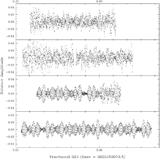
Figure 3: Left panel: Optical (“white light”) light curves of PG 1219+534 obtained at CFHT between 2004, March $9-12$ (top to bottom slices). The light curves are expressed in terms of residual amplitude relative to the mean brightness of the star. Right panel: Fourier amplitude spectra (given as a percentage of the mean brightness of the star) in the $0-20$ mHz bandpass associated with each light curve shown in the left panel.

We observed PG~1219+534 in optical “white light” fast photometric mode at the CFHT during a dedicated four night run scheduled on 2004, March. Table 1 provides a journal of these observations. As with our previous programs, the photometric data were gathered with Lapoune, the portable Montréal three-channel photometer. The data were then carefully corrected for various undesirable effects (e.g., atmospheric transparency variations, extinction, etc.) using the data reduction package Oscar specifically designed by one of us (P.B.) for that purpose. We refer the interested reader to Billères et al. (1997) for details on the observations and data reduction procedures.

The observing conditions varied from relatively poor for the first two nights to simply outstanding for the rest of the run. The quality of the data gathered during these observations is illustrated on a night-by-night basis in Figure 3, where the left panel shows the fully reduced light curves, and the right panel displays the corresponding Fourier amplitude spectra in the relevant $0-20$ mHz frequency bandpass. The light curves from the first and second nights (runs cfh-104, cfh-105a and cfh-105b), as well as from the very end of the third night (run cfh-106b) were rather noisy, and this is also clearly reflected in their associated Fourier amplitude spectra. These time series were obtained during bright time (contrary to our request) and the presence of dust and high winds as well as thin cirrus during the first two nights is responsible for the much lower quality of the data we obtained. Our past experience at the CFHT shows that photometric data gathered with Lapoune can be quite good even in presence of thin cirrus, but this works only under dark sky conditions. The contrast is particularly sharp when comparing these data with the very high quality photometry (more typical of what we have been accustomed to at CFHT) acquired during most of the third night (run cfh-106a) and during the fourth night (run cfh-107), where conditions became photometric. That last light curve in particular, a chunk of 9.36 h with no interruption obtained during perfectly photometric conditions, is among the best that have been obtained with Lapoune at CFHT, so far. It is shown in greater detail in Figure 4. The variations have typical peak-to-peak amplitudes of less than $\sim 6\%$ and are dominated by a pseudo-period of $\sim 130$ s. It is obvious however that several other periodicities are involved in the variations, considering the strong beating structures that can be seen in the light curve and which are typical of destructive and constructive interferences between modes. The multiperiodic nature of the variations is, of course, confirmed in the Fourier amplitude spectra shown in the right panel of Figure 3, where four dominant peaks clearly emerge over the mean noise level. Our thorough analysis of the light curves described in the following section will reveal that even more periodicities, indeed, contribute to the luminosity variations seen in PG~1219+534.

Figure 4: Expanded view of the best optical light curve obtained on PG 1219+534 during the night of 2004, March 12. Each band covers an interval of 4,000 s and the amplitude is expressed in terms of the residual relative to the mean brightness of the star.

3 Analysis of the Light Curves

Figure 5: Fourier amplitude spectrum and residuals after prewhitening of the identified periods (frequencies) in the time series of the four nights analyzed separately (night 1, 2, 3 and 4, from upper-left panel to lower-right panel, respectively). For night 3 (lower-left panel), only the best part (run cfh-106a) of the light curve has been considered. The dashed (dotted) line refers to a value equal to 3.7 (3.0) times the mean noise level.

Considering that the quality of the light curves obtained on PG~1219+534 during our CFHT run is particularly inhomogeneous, we carried out detailed frequency analyses on various subsets of the observations. We analyzed the time series in a standard manner by combining Fourier analysis, least-squares fits to the light curves, and prewhitening techniques. The procedure to extract pulsation modes from the light curves is now greatly eased by a new dedicated software named Berthe, developed recently by one of us (P.B.). This software provides efficient tools to conveniently proceed along the procedure described below.

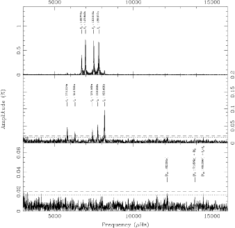
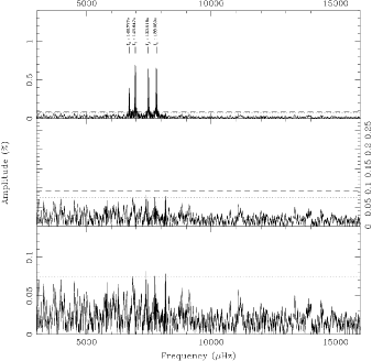
Figure 6: Same as Figure 5, but for the combined time series from night 3 (run cfh-106a only) and night 4 (left panel), and for all light curves assembled together (right panel).

The first step of the procedure is to compute the Fourier transform of the light curve. We typically use 10,000 frequency points per chunk of width 1 mHz in the Fourier space, which largely oversamples that domain. The upper slices in the panels shown in Figure 5 and Figure 6 illustrate the Fourier spectrum of the light curves of PG~1219+534 in the relevant 3-16 mHz bandpass. As noted previously, the light curve shows multiperiodic harmonic oscillations which is reflected through the presence of multiple peaks in the Fourier spectrum. We next isolate from the Fourier spectrum the frequency (period) of the usually (but not always) largest peak seen in a given frequency interval. That frequency (period) is used in a least-squares routine that provides the amplitude and the phase of the harmonic oscillation of that given period which best-fits the complete light curve. This harmonic oscillation is then subtracted from the light curve in the time domain (prewhitening) and the Fourier transform of the residual light curve is computed. A second frequency, again often associated with the highest peak in the Fourier transform of the residual, is identified and the least squares routine is reapplied but this time with the two frequencies, amplitudes, and phases fitted simultaneously. This provides upgraded estimates for the amplitude and phase of the first harmonic oscillation and initial estimates for the second one. These two harmonic oscillations are then subtracted from the original light curve through prewhitening and another Fourier transform of the residual light curve is computed. The procedure is repeated until no useful information can be extracted from the residual light curve through this method. It is standard to stop the iteration when the amplitude of the candidate peaks in the Fourier domain gets below 3.7 times the local rms noise level, which corresponds to the 99% statistical significance limit. We find, in practice, that applications of more sophisticated statistical methods to test for the reality of peaks in the Fourier domain (such as the false-alarm probability formalism) generally confirm that an amplitude 3 times larger than the mean noise level is sufficient to account for the reality of a mode.

Table 2: Periods of the Modulations Detected in the Light Curves of PG 1219+534.

	Koen et al.	Night	Night	Night	Night	Nights	Nights	Nights
	1999	1	2	3	4	1 & 2	3 & 4	All
Resolution ($\mu$Hz)	3.64	45.02	35.03	62.11	29.68	8.85	8.61	3.44
Duty cycle (%)	17.8	100	98.3	100	100	44.5	42.9	34.4
FT Noise (%)	0.040	0.040	0.055	0.0090	0.0040	0.040	0.0055	0.025
	Period	Period	Period	Period	Period	Period	Period	Period
Id.	(s)	(s)	(s)	(s)	(s)	(s)	(s)	(s)
$f_{7}$	…	…	…	172.241	172.164	…	172.214	…
$f_{9}$	…	…	…	159.046	158.793	…	158.789	…
$f_{4}$	148.776	148.603	148.831	148.796	148.776	148.769	148.775	148.777
$f_{2}$	143.649	143.619	143.585	143.639	143.650	143.652	143.649	143.647
$f_{8}$	[134.960]	…	…	134.962	135.147	…	135.160	…
$f_{3}$	133.510	133.497	133.490	133.519	133.517	133.503	133.516	133.518
$f_{6}$	…	…	…	129.239	129.130	…	129.099	…
$f_{1}$	128.078	128.115	128.104	128.069	128.079	128.075	128.077	128.080
$f_{5}$	…	…	…	122.404	122.397	…	122.408	…
$[f_{10}]$	…	…	…	…	[82.292]	…	[82.261]	…
$[f_{11}]$	…	…	…	…	[71.865]	…	[71.879]	…
$[f_{12}]$	…	…	…	…	[69.193]	…	[69.204]	…

We first analyzed the light curves obtained on PG~1219+534 separately, on a night-by-night basis, before combining them according to their respective mean noise level, i.e., night 1 was combined with night 2, and night 3 (without the noisy chunk at the end of the night that would just ruin the signal-to-noise ratio, if added) was combined with night 4. Finally, we examined the complete light curve built from all nights. For the various cases considered, illustrations of the Fourier transforms obtained before and after prewhitening of the identified frequencies are provided in Figure 5 and Figure 6. The periods extracted from these analyses are listed in Table 2 (each identified period is labeled $f_{j}$, where $j$ is ordered by decreasing amplitude), as well as the results obtained previously by Koen et al. (1999). In this table, we also provide information relative to the run considered. This includes the resolution achieved (in $\mu$Hz), the rms noise level reached in the data (in $\%$ of the mean brightness of the star), and the duty cycle (in % of the total coverage). Of course, each night considered individually gives a duty cycle of $100\%$ (except for the second night, due to a short interruption in the time series), which then decreases due to the daily gaps that are introduced when data sets of successive nights are combined (down to 34.4% for the whole run). In the meantime, however, the frequency resolution improves from 29.7 $\mu$Hz for our longest contiguous light curve (night 4) down to 3.44 $\mu$Hz with the time baseline of the whole photometric run. We note that the best frequency resolution reached with our data set is comparable to the resolution obtained in Koen et al. (1999), but our coverage is better. Unfortunately, no significant improvement of the mean noise level in the Fourier space can be achieved with the whole data set compared to Koen et al. (1999) data. This is a direct consequence of the heterogeneous quality of the CFHT light curves. The rms noise level in the Fourier domain is approximately $5-10$ times higher for the first two nights compared to the excellent data obtained during nights 3 and 4. Mixing all time series to construct the global light curve significantly degrades the S/N ratio in the Fourier domain, as the mean noise level is essentially regulated by the light curve of worst quality. Obviously, in the present case, focussing on the best data only (i.e., those obtained during night 3 and night 4) would yield the best results for extracting pulsation modes from PG~1219+534 photometric variations.

The light curve from the fourth night is by far the best obtained during these observations and thus, not surprisingly, gives the Fourier transform with the lowest rms noise level ($\sim 0.004\%$). From that time series alone, 9 frequencies (periods) could be extracted without any ambiguity. The prewhitening sequence for this particular light curve is illustrated in the successive bands shown in the lower-right panel of Figure 5. The upper band displays the full amplitude spectrum in the relevant $3-16$ mHz frequency bandpass where photometric activity is concentrated. We note that from 16 mHz up to the Nyquist frequency (50 mHz, as we used a sampling time of 10 s), the structures found in the Fourier amplitude spectrum are entirely consistent with noise. At the low frequency end, the rms noise level increases due to residual atmospheric variations (which are difficult to remove completely) and no obvious periodicities could be identified (but see below). Four dominant periods, labeled $f_{1}$ to $f_{4}$, are clearly seen at that stage, while the noise level is so low at the provided scale that it is essentially invisible. The mid-band shows the Fourier transform of the residual light curve after prewhitening of those four main harmonic oscillations. This leads to the unambiguous detection of five additional periods ($f_{5}$ to $f_{9}$) that clearly emerge above the detection threshold of 3.7 times the rms noise level materialized by the horizontal dashed line (the dotted line indicates the limit of 3 times the rms noise level). The lower band displays the Fourier transform of the residual light curve after prewhitening of the nine identified periodicities. Little power is then left in the Fourier transform of the residual light curve, but hints of remaining structures exist, in particular at the high-frequency end of the bandpass considered. Three more structures ($f_{10}$, $f_{11}$, and $f_{12}$) are indeed found slightly above, or just below the detection threshold (dashed line). These are also visible in the Fourier transform of the residual light curve of the combined nights 3 and 4 (lower-band in left-panel of Figure 6), but unfortunately cannot be confirmed with the analysis of the other light curves, due to their much higher mean noise level. For this reason, we consider as marginal the detections of these periods, although we will provide below arguments which suggest that these structures may be real. These marginal period detections are indicated within brackets in Table 2.

Table 3: Properties of the Harmonic Oscillations Identified in PG~1219+534.

	Frequency	Period	Amplitude	Phase	Comments
Id.	($\mu$Hz)	(s)	(%)	(s)
$f_{7}$	5806.71	172.214	$0.0456\pm 0.0030$	$68.72\pm 1.80$
$f_{9}$	6297.65	158.789	$0.0334\pm 0.0030$	$23.14\pm 2.27$
$f_{4}$	6721.55	148.775	$0.4053\pm 0.0030$	$42.86\pm 0.18$	detected with an amplitude of 0.22% by Koen et al. (1999)
$f_{2}$	6961.39	143.649	$0.7228\pm 0.0030$	$102.50\pm 0.09$	detected with an amplitude of 0.18% by Koen et al. (1999)
$f_{8}$	7398.62	135.160	$0.0429\pm 0.0030$	$98.73\pm 1.51$
$f_{3}$	7489.73	133.516	$0.6874\pm 0.0030$	$43.65\pm 0.09$	detected with an amplitude of 0.23% by Koen et al. (1999)
$f_{6}$	7745.98	129.099	$0.0544\pm 0.0030$	$104.69\pm 1.13$
$f_{1}$	7807.79	128.077	$0.7972\pm 0.0030$	$44.07\pm 0.08$	detected with an amplitude of 0.85% by Koen et al. (1999)
$f_{5}$	8169.43	122.408	$0.0963\pm 0.0030$	$95.70\pm 0.61$
$[f_{10}]$	[12156.40]	[82.261]	[$0.0190\pm 0.0030$]	[$59.38\pm 2.07$]	slightly above detection threshold; not used for seismology
$[f_{11}]$	[13912.31]	[71.879]	[$0.0143\pm 0.0030$]	[$21.06\pm 2.40$]	$2f_{2}$; not used for seismology
$[f_{12}]$	[14450.08]	[69.204]	[$0.0188\pm 0.0030$]	[$48.10\pm 1.76$]	$f_{2}+f_{3}$; not used for seismology

Globally, we find that the four dominant modes, $f_{1}$ to $f_{4}$, are detected in all the CFHT light curves (and combinations of light curves) and correspond to the four periods already identified in Koen et al. (1999). These authors had also suspicions concerning a fifth period at 134.96 s (that corresponds to $f_{8}$, here), which we indeed confirm with no ambiguity on the basis of the best light curves we obtained. Note that only the four dominant periods are seen when nights 1 and 2 are considered either separately or combined into larger data sets, such as the complete light curve built from all nights. This is due, again, to the relatively poor quality of these specific data and the dramatic impact it has on the mean noise level in the Fourier domain. Nonetheless, the analysis of the best available time series yields a significant improvement in terms of the number of modes detected compared to the original data, since five additional periods ($f_{5}$ to $f_{9}$) can be securely identified in the spectrum of PG~1219+534.

We provide in Table 3 a list of the detailed properties that characterize the nine harmonic oscillations uncovered. These are the frequency (in $\mu$Hz), the period (in second), the amplitude (in % of the mean brightness), and the phase (in seconds). The three marginal detections mentioned above are also included within brackets. We note that two of these can be interpreted as harmonics or cross-frequencies of the dominant peaks, i.e., $f_{11}=2f_{2}$ and $f_{12}=f_{2}+f_{3}$ (and therefore would not constitute independent modes usable for asteroseismology), while the third period $(f_{10}$) may be an independent pulsation mode. We have, however, explicitly excluded this period and considered only the nine well secured pulsation modes for the following asteroseismic analysis of PG~1219+534. We have adopted the list of periods derived from the analysis of the combined light curves from night 3 and night 4, which allows to recover all the harmonic oscillations seen in the data taken during night 4 treated separately (the best achievement in terms of S/N ratio) while reaching a decent frequency resolution of 8.61 $\mu$Hz. The measured frequencies (each associated with a frequency peak in the Fourier domain) are probably accurate to 1/10 of the formal resolution (itself corresponding to the width at half-maximum of such a peak), i.e., to within 0.86 $\mu$Hz (see Bretthorst, 1988). The amplitudes and phases derived through the least-squares technique have formal errors as given in Table 3. We note at this point, that the gain in frequency resolution obtained while combining all light curves for the Fourier analysis does not reveal the presence of close frequencies near the dominant peaks (due to rotational splitting, for instance). This observation holds for the five newly discovered frequencies as well, although the frequency resolution is lower in these cases. Such a finding indicates that PG~1219+534 is likely a slow rotator with a rotation period longer than $\sim 3.4$ days, i.e., the longest time baseline achieved with the photometry currently available. Finally, we note a significant change in the amplitude of three of the four dominant periods that have been detected in both our contemporary data and the older Koen et al. (1999) light curves. Except for the period $f_{1}$ which is found slightly weaker (by $\sim 6\%$) in our time series, the periods $f_{2}$, $f_{3}$, and $f_{4}$ all appear much stronger than observed in Koen et al. (1999), by factors up to $\sim 2-4$. Such amplitude variations are not uncommon among rapidly pulsating sdB stars. In PG~1219+534, these may be due to beating between very close – thus, unresolved with current data – frequencies (multiplet components caused by slow rotation, for instance), and/or to significant changes in the intrinsic amplitudes of the modes themselves. However, additional observations with longer time baselines will be needed to further discuss the stability of pulsation mode amplitudes in this star.

Interestingly, the odd conditions under which the CFHT data were obtained provides us with a perfect illustration of the fact that mixing low and high S/N ratio time series can essentially ruin all the benefit of having the high-sensitivity data. The overall mean noise level in the Fourier space is clearly mostly regulated by the noise level of the worst light curve included in the analysis. It is instructive that, for this particular star PG~1219+534 which, at the outset, turns out to have a relatively simple and well resolved pulsation spectrum, just one night of high sensitivity CFHT data appears to be sufficient to make this object amenable to detailed asteroseismic analysis. More generally, for the purpose of asteroseismology of stars with simple enough oscillation spectra (such as EC14026 stars often have, with some exceptions), high sensitivity is often to be sought preferrentially to frequency resolution and/or coverage. This, indeed, has some implications for the treatment of multisite campaign data where light curves of various quality are generally mixed. In those cases, mixing low S/N data with high S/N data, although improving resolution and reducing aliasing problems, can significantly degrade the S/N ratio reached with the best available data. Accordingly, weighting techniques may contribute, in some circumstances, to reduce the deterioration of the overall S/N ratio, although generally at the expense of a degraded window function (see, for instance, the discussion of Handler 2003). However, with very heterogeneous data sets, these techniques would still lead to a significant increase of the mean noise level in the Fourier domain compared to the S/N ratio achieved with the best light curves. This has to be considered carefully when the goal is to extract low amplitude variations to increase the number of modes for asteroseismology. Of course, the best is to have both high sensitivity and coverage with data as homogeneous as possible. Along this line, we hope for future bi- (or tri-) site fast photometric observations based on 4m-class telescopes, as it would constitute, in addition to other developing techniques (multicolor photometry and high time resolution spectroscopy), a significant step forward in the field of asteroseismology of EC14026 stars.

To end this Section, let us briefly mention that, while performing the Fourier analysis of the best light curves obtained on PG~1219+534, we have discovered hints of low frequency modulations in the amplitude spectrum. Having a closer look at the highest S/N ratio Fourier amplitude spectra shown in the right panel of Figure 3 (especially the lowest band corresponding to the data of our best night), one can notice low amplitude structures below 1 mHz that still significantly emerge above the local mean noise level. If such periodic modulations are real and due to pulsations, those peaks would correspond to modulations with periods much longer than the typical periods observed in EC 14026 stars, thus involving relatively high-order gravity modes. To some extent, it would be similar to the variations seen in the long period sdB pulsators, although PG~1219+534 does not have, in principle, the expected physical parameters to belong to that class of pulsating stars which, typically, have much lower effective temperatures and surface gravities. A possible analogy would be with the recent exciting discovery of a long-period photometric variation in the EC14026 star HS 0702+6043 (Schuh et al., 2005) which suggests that this star may pulsate in both low-order $p$-modes and high-order $g$-modes. It is, however, premature to speculate further on the nature of these (potential) low frequency luminosity modulations in PG~1219+534. Additional photometric observations at high sensitivity with a longer time baseline than is currently available will be necessary to address this particular issue and possibly confirm (or rule out) the presence of $g$-modes in PG~1219+534. Specific efforts along this line are underway.

4 Asteroseismic Interpretation of the Observations

4.1 The Double-Optimization Scheme

The asteroseismological interpretation of the period spectrum of pulsating stars has often been impaired by the lack of identification of the modes being observed. The analysis of EC14026 stars is confronted to similar challenges as white light fast photometry generally gives little clue – and quite often no clue at all – about the degree $\ell$ and/or radial order $k$ of the modes detected. Indeed, for PG 1219+534, we have no a priori knowledge of the geometry of the nine observed modes (not even hints on the $\ell$ value, since no splitting due to rotation has been detected at the current frequency resolution). Nonetheless, we have pursued major efforts in the last few years to develop a new method that allows us to bypass this difficulty.

Our approach is based on the well known forward method which consists of comparing directly periods computed from stellar models to periods observed in the star under consideration with the goal of reproducing as accurately as possible its oscillation spectrum. Applied to EC14026 stars, it consists of a double-optimization procedure that takes place simultaneously at the period matching level and in the model parameter space. Due to the lack of mode identification from the available data, assigning $N_{o}$ observed periods to $N_{t}$ theoretical periods from a given model ($N_{t}>N_{o}$, in general) usually leaves a myriad of possible combinations. The first optimization therefore consists of finding the combination (or mode identification) that leads to the best possible simultaneous match of all the observed periods for that given model. We note that this best match does not necessarily have to be a good match at this point. This will be the role of the second optimization procedure discussed below. More formally, the quality (or merit) of a period fit is evaluated as the sum of the squared differences $\chi^{2}$ between the observed periods and their assigned theoretical periods (i.e., through a least-squares formalism). The chosen mode identification for a given model is then the combination that provides a $\overline{\chi}^{2}$ value corresponding to the minimum of that sum among all the possible associations, that is

$$\overline{\chi}^{2}\equiv\min\left\{\chi^{2}=\sum_{i=1}^{N_{o}}\left(\frac{P_{{\rm obs}}^{(i)}-P_{{\rm th}}^{(i)}}{\sigma_{i}}\right)^{2}\,,\,\forall\,\,{\rm combinations}\right\}.$$ (1)

Here, $P_{{\rm obs}}^{(i)}$ is the $i^{{\rm th}}$ observed period and $P_{{\rm th}}^{(i)}$ represents its associated theoretical period. $\sigma_{i}$ is an optional weight that can be attributed either individually on periods or globally (see Subsection 4.3). The second optimization is carried out in the model parameter space where the quantity $\overline{\chi}^{2}$ derived from the first optimization is now seen as a function of the $N$ model parameters (considering here the general case), i.e., $\overline{\chi}^{2}\equiv\overline{\chi}^{2}(a_{1},a_{2},...,a_{N})$, where $a_{i}$ represents one of the $N$ parameters. The procedure then consists of localizing the optimal model (or models) that minimizes this “merit” function in the $N$-dimensional space, leading objectively to the best period match of the observations.

We have developed various sets of numerical tools that allows us to apply this double-optimization scheme to isolate best period fitting models for asteroseismology. Our original efforts along those lines were described in Brassard et al. (2001). Since then, many important improvements have been made and two independent packages (fortunately leading to the same results!) are now operational, one in Montréal and the other in Toulouse. Detailed descriptions of the numerical tools developed in these packages will be reported elsewhere. Briefly, the Toulouse package extensively used for this analysis of PG~1219+534 includes a genetic algorithm based period matching code that performs the first optimization part, a parallel grid computing code useful to explore the parameter space and visualize the complex shape of the $\overline{\chi}^{2}(a_{1},a_{2},...,a_{N})$ function, and a parallel multimodal genetic algorithm based optimization code designed to explore efficiently the vast $N$-dimensional parameter space and seek for the optimal solutions. By locating simultaneously the global and local minima of the $\overline{\chi}^{2}$ function, this code is capable of identifying several optimal models if more than one solution exists.

It is important to realize that this approach is in fact built on the very simple requirement that models pretending to provide a good asteroseismological fit of the spectrum of a pulsating star must match all the observed periods simultaneously, i.e., the procedure is a global optimization. Moreover, we stress that the solutions identified from this approach do not rely on any previous mode identification. The mode identification appears instead naturally as the solution of the global fitting procedure, i.e., the mode identification obtained is the one that provides the best simultaneous match of all the detected periods.

4.2 Equilibrium Models and Computations of their Pulsation Properties

Applications of our double-optimization scheme to EC14026 stars requires computing appropriate theoretical period spectra that need to be compared with the observed periods. Three codes are involved in this process, starting with an equilibrium model building code first described in Brassard & Fontaine (1994) and adapted to produce the so-called “second generation” models suitable for pulsating sdB stars (see Charpinet et al., 1997, 2001). These models are improved static envelope structures extending as deep as $\log q=\log[1-M(r)/M_{*}]\simeq-0.05$. For the purpose of pulsation calculations, the central missing nucleus that contains $\sim 10\%$ of the stellar mass is treated as a “hard ball”. This approach, in comparisons to full evolutionary stellar models, gives excellent pulsation results, especially for the relatively shallow $p$-modes that are, in hot B subdwarf stars, insensitive to the detailed structure of the central parts of the core as was discussed at length in Charpinet (1999) and Charpinet et al. (2000, 2002). Moreover, these “second generation” static models are superior to all evolutionary structures currently available in that they incorporate the nonuniform iron abundance profiles predicted by the theory of microscopic diffusion assuming an equilibrium between gravitational settling and radiative levitation. We recall that diffusion leads to the constitution of a reservoir of iron in the H-rich envelope of subdwarf B stars with significant iron enrichments produced locally which are responsible, through the $\kappa$-mechanism, for the destabilization of the low-order, low-degree $p$-modes observed in EC14026 pulsators (Charpinet et al., 1997). This additional ingredient in the constitutive physics of the models is therefore essential to reproduce the excitation of the pulsation modes. In addition, microscopic diffusion modifies sufficiently the stellar structure to induce significant changes to the pulsation periods themselves, thus impacting on the asteroseismic analysis. Consequently, radiative levitation is a crucial ingredient that must be taken into account in the modeling of pulsating sdB stars for the purpose of accurate asteroseismology. Four fundamental parameters are required to specify the internal structure of hot B subdwarf stars with the second-generation models: the effective temperature $T_{{\rm eff}}$, the surface gravity $\log g$ (traditionally given in terms of its logarithm), the total mass of the star $M_{*}$, and the logarithmic fractional mass of the hydrogen-rich envelope $\log q({\rm H)\equiv}\log[M({\rm H})/M_{*}]$. The latter parameter is intimately related to the more familiar parameter $M_{{\rm env}}$, which corresponds to the total mass of the H-rich envelope.

In a second step, we use two efficient codes based on finite element techniques to compute the pulsation properties of the model. The first one is an updated version of the adiabatic code described in detail in Brassard et al. (1992). It is used as an intermediate (and necessary) step to obtain estimates for the pulsation mode properties (periods and eigenfunctions) that are then used as first guesses in the solution of the full, nonadiabatic set of nonradial oscillation equations. The second one is an improved version of the nonadiabatic code that has been described briefly in Fontaine et al. (1994) and which solves the nonadiabatic eigenvalue problem. It provides the necessary quantities to compare with the observations. For the purpose of asteroseismology, these are mainly the periods and the stability coefficients. To illustrate the type of quantities that are derived from the whole process, we provide, in Table 4, a typical output of the nonadiabatic pulsation code that gives the pulsation properties of a given model. While it refers specifically to the optimal model (see the discussion in the next subsection), we only wish to emphasize the illustrative aspect of the theoretical results at this point. For each mode found in the chosen period interval, Table 4 gives the degree $\ell$, the radial order $k$, the period $P_{{\rm th}}$ ($=2\pi/\sigma_{R}$, where $\sigma_{R}$ is the real part of the complex eigenfrequency), the stability coefficient $\sigma_{I}$ (the imaginary part of the eigenfrequency), the logarithm of the so-called kinetic energy of the mode $E$, and the dimensionless first-order solid rotation coefficient $C_{kl}$. As is standard, our equilibrium stellar models are perfectly spherical, and each mode is $2l+1$ fold-degenerate in eigenfrequency.

For asteroseismic studies, the most important quantities derived from theoretical calculations are of course the periods of the modes. These are sensitive to the global structural parameters of a model which we seek to infer for a real star through a comparison with a set of observed periods. Because nonadiabatic effects on the periods are small (but included in our calculations), asteroseismology could very well be carried out at the level of the adiabatic approximation only. However, the stability coefficient, a purely nonadiabatic quantity, also provides useful information on the mode driving mechanism. A positive value of $\sigma_{I}$ indicates that a mode is damped (or “stable”), and therefore that it should not be observable. A negative value of $\sigma_{I}$ indicates that the mode is excited (or “unstable”) in the model, and consequently that it may reach observable amplitudes. As illustrated in Table 4, modes are excited within a band of periods associated with low-order acoustic modes. This is typical of all our models of rapid sdB pulsators. In terms of asteroseismology, it is of course within that bandpass that one would expect to find the observed periods of a real EC14026 star and this important stability information justifies the use of full nonadiabatic calculations in our case. For its part, the kinetic energy is a secondary quantity in the present context. It provides a measure of the required energy to excite a mode of a given amplitude at the surface of a star. Since this is a normalized quantity, only its relative amplitude from mode to mode is of interest. The kinetic energy is a useful diagnostic tool for determining where pulsation modes are formed. Larger values of $E$ imply that such modes probe deeper into the star, in higher density regions. The kinetic energy bears the signature of mode trapping/confinement, which are caused by partial reflexions of propagating waves onto thin chemical transition zones (between the pure He-core and the H-rich envelope, mainly). Finally, the rotation coefficient is useful for interpreting the fine structure in the Fourier domain in terms of slow rotation that lifts the $2\ell+1$ fold-degeneracy of the mode periods. At the frequency resolution reached in our observations of PG~1219+534, no such structures have been detected, however.

4.3 The Quest for the Optimal Model of PG 1219+534

The search for the optimal model solution (or solutions) that can best reproduce the nine identified periods of PG~1219+534 was initiated with our multimodal genetic algorithm (GA) optimization code. As mentioned briefly in the previous subsection, the search is carried out in the four-dimensional space defined by the main parameters $T_{{\rm eff}}$, $\log g$, $M_{*}$, and $\log q({\rm H})$ that specify the structure of a sdB star with our second-generation models. The GA code, designed for efficient explorations of a wide parameter space domain, was first used to localize potential regions were solutions may exist. For that purpose, initial boundaries of the search domain were defined as follows : 37,000 K $\geq T_{{\rm eff}}\geq$ 28,000 K, $5.65\leq\log g\leq 5.95$ for the surface parameters, and $-5.0\leq\log q({\rm H})\leq-2.0$, $0.30\leq M_{*}/M_{\odot}\leq 0.53$ for the structural parameters.

These limits were loosely set according to current spectroscopic estimates for the atmospheric parameters $T_{{\rm eff}}$ and $\log g$ of PG~1219+534. We emphasize the fact that any eventual determination of the atmospheric parameters of PG~1219+534 through asteroseismic means has to be consistent with our spectroscopic estimates. Since the latter are based on standard, well-understood techniques (see, however, the discussions of Wesemael et al. 1997 and Heber & Edelmann 2004 on possible systematic errors introduced by these methods when applied to sdB stars), the validity of our pulsating models would have to be questioned if the results show otherwise. Constraints on the two other parameters $M_{*}$ and $\log q({\rm H})$ rely on stellar evolution theory. The evolutionary calculations of Dorman et al. (1993) indicate that hot B subdwarfs are core helium burning stars on the Extreme Horizontal Branch that evolve as “AGB-Manqué” objects. According to these calculations, their possible masses are found in a narrow range $0.40-0.43\lesssim M_{*}/M_{\odot}\lesssim 0.53$, with a somewhat uncertain lower limit related to the minimum mass required to ignite helium and a more sharply defined upper limit above which the models evolve to the AGB. More recently, however, Han et al. (2003) suggested, in their investigation of various binary evolution scenarios for the formation of sdB stars, a somewhat larger distribution of masses among these stars. Although these authors derived mass distributions which are strongly peaked around the canonical value of $\sim 0.47$ $M_{\odot}$, they suggest that the mass of an sdB star could be as low as $\sim 0.30$ $M_{\odot}$ if formed through the Roche lobe overflow channel or as high as $\sim 0.70$ $M_{\odot}$ if formed through the merger channel. To explore these possibilities with asteroseismology, we adopted a generous lower mass limit of $0.30$ $M_{\odot}$ but kept $0.53$ $M_{\odot}$ as our upper boundary (results from test calculations for models with higher masses will be briefly discussed, though). Finally, the range of possible values for the last parameter $\log q({\rm H)}$, which is related to the mass of the H-rich envelope, was chosen according to the work of Dorman et al. (1993) in order to fully map the region of the $\log g-T_{{\rm eff}}$ plane where sdB stars are found.

For the pulsation calculations step, we considered all the modes (be it of $p$-, $f$-, or $g$-type) of degree $\ell=0$ up to $\ell=3$ with periods in the range $70-500$ s, i.e., covering amply the range of periods observed in PG~1219+534. The usual argument to limit the value of $\ell$ above which modes are no longer observable is geometric cancellation on the visible disk of the star. A quantitative expression of the visibility argument used to restrict the search to low values of $\ell$ is obtained by evaluating numerically the geometric factor given, for example, by equation (B7) of Brassard et al. (1995). Using an Eddington limb darkening law in that formulation gives visibility factors with values of 1.000, 0.7083, 0.3250, 0.0625, 0.0208, 0.0078, 0.0078, 0.0023, 0.0039, 0.0009, 0.0023, 0.0005, and 0.0015, respectively, for $\ell=0$, 1, 2, 3, 4, 5, 6, 7, 8, 9, 10, 11, and 12. This cancellation effect naturally favors a priori values of $\ell=0$, 1, and 2 in pulsating stars in general. We note, however, that the mode densities and period distributions seen in several well-observed EC14026 stars such as KPD 1930+2752, PG 1605+072, PG 1047+003, and PG 0014+067 force us to consider modes with higher $\ell$ values ($\ell=3$, or even $\ell=4$ in some cases). Otherwise, there would be not enough theoretical modes available in the observed period window to account for the observations. To justify further the (small) heresy that consists of considering modes of degree up to $\ell=3$ or 4 (although, again, observational evidence already suggests that such modes are effectively seen), we stress that our growing observational experience with EC14026 pulsators indicates clearly that intrinsic mode amplitudes in these stars are not the same from mode to mode. In addition, these amplitudes may vary significantly on a monthly or yearly basis, some modes being visible one season but disappearing the next one. Therefore, one should be cautious with the simple geometric cancellation argument which is based on the implicit assumption that intrinsic amplitudes of all modes are the same. We suggest instead, at least for EC14026 stars, that the limit in $\ell$ at which modes cease to be observable due to cancellation effects cannot be a strict threshold, since it also depends on the intrinsic amplitude of the modes considered individually. For the purpose of asteroseismology, we choose to consider modes from $\ell=0$ up to the minimum value of the degree $\ell$ needed to account for the mode density in the observed period range. For the PG~1219+534 periods identified in Table 3, modes up to $\ell=3$ are needed. Of course, we cannot rule out completely the presence of the odd $\ell=4$ modes (or perhaps even a mode of higher degree) with an unusually high intrinsic amplitude in the light curve of PG~1219+534. Our approach explicitly excludes this possibility, however, and we seek to interpret the period distribution in that star solely in terms of $\ell=0-3$ modes.

Within the search domain specified, the GA code identified two families of solutions that best match the observed periods. A third family of potential solutions was also spotted near the low-gravity edge of the search domain, but was immediately rejected as being highly inconsistent with the available spectroscopic measurements (see discussion below). These model solutions are essentially equivalent in terms of quality of fit, indicating that best-fitting the observed periods only leads to a degenerate situation (there is another source of solution degeneracy which will be discussed below). The optimal model corresponding to the first family of solutions was found at $T_{{\rm eff}}=$ 33,640 K, $\log g=5.8071$, $\log q({\rm H})=-4.3448$, and $M_{*}=0.4570$ $M_{\odot}$ with a $\overline{\chi}^{2}$ value of 0.0784. The model associated with the second family of solutions was localized at $T_{{\rm eff}}=$ 33,715 K, $\log g=5.7178$, $\log q({\rm H})=-3.8142$, and $M_{*}=0.4680$ $M_{\odot}$ with a $\overline{\chi}^{2}$ value of 0.0878. Note that in the evaluation of $\overline{\chi}^{2}$, we have chosen a global weight factor $\sigma_{i}=\sigma$, where $\sigma$ is the inverse of the theoretical mode density, i.e., the ratio of the width of the period window (here $500-70=430$ s) to the number of theoretical modes in that window for a given model. This choice was made in order to ease the automatic search of the best-fit models in the parameter space by offsetting, at least in part, the built-in bias in favor of models with a higher theoretical mode density (generally, the models having a lower surface gravity). Of course, this choice does not influence the positions of the minimum values of $\overline{\chi}^{2}$ in the parameter space domain. Maps displayed in Figure 7 and Figure 8 illustrate the complex shape of the $\overline{\chi}^{2}$-function (shown as isocontours of constant value of $\log\overline{\chi}^{2}$) in the vicinity of the two potential solutions, whose exact locations according to the GA code are indicated by black crosses. These figures respectively show slices of this function along the $\log g-T_{{\rm eff}}$ plane (at fixed parameters $M_{*}$ and $\log q({\rm H})$ set to their optimal values) and along the $M_{*}-\log q({\rm H})$ plane (at fixed parameters $T_{{\rm eff}}$ and $\log g$ set to their optimal values). Best fitting models corresponding to low values of $\overline{\chi}^{2}$ appear as dark blue regions, while red areas indicate regions of the model parameter space with high values of $\overline{\chi}^{2}$, i.e., where theoretical periods computed from models do not fit well the observed periods. Considering the logarithmic scale used to represent the merit function on these plots, we point out that the blue regions correspond to well-defined minima.

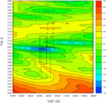
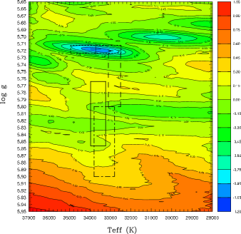
Figure 7: Left panel: Slice of the $\overline{\chi}^{2}$-function (in logarithmic units) along the $\log g-T_{{\rm eff}}$ plane at fixed parameters $M_{*}$ and $\log q({\rm H})$ set to their optimal values found for the first best-fit model solution ($M_{*}=0.4570$ $M_{\odot}$ and $\log q({\rm H})=-4.3448$). The solid-line rectangle shows our spectroscopic estimate with its uncertainties for the atmospheric parameters of PG~1219+534, while the dashed-line and dashed-dotted-line rectangles represent the Koen et al. (1999) and Heber et al. (2000; from NLTE H+He model atmospheres) spectroscopic measuremen ts, respectively. The dotted-line rectangle shows the estimated error box associated with our asteroseismic determination of the parameters $\log g$ and $T_{{\rm eff}}$ (see text). The black cross indicates the position of the best-fit solution. Right panel: Same as left panel but for the second best-fit model solution (the fixed parameters are set to the optimal values $M_{*}=0.4680$ $M_{\odot}$ and $\log q({\rm H})=-3.8142$).

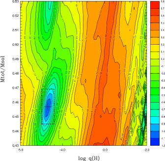
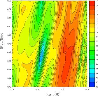
Figure 8: Left panel: Slice of the $\overline{\chi}^{2}$-function (in logarithmic units) along the $M_{*}-\log q({\rm H})$ plane at fixed parameters $T_{{\rm eff}}$ and $\log g$ set to their optimal values found for the first best-fit model solution ($T_{{\rm eff}}=$ 33,640 K and $\log g=5.8071$). The dotted-line rectangle shows the estimated error box associated with our asteroseismic determination of the parameters $\log q({\rm H})$ and $M_{*}$ (see text). The black cross indicates the position of the best-fit solution considered. Right panel: Same as left panel but for the second best-fit model solution (the fixed parameters are set to the optimal values $T_{{\rm eff}}=$ 33,715 K and $\log g=5.7178$).

If one family of solutions among the two identified cannot be preferred over the other one simply on the basis of the $\overline{\chi}^{2}$ value alone, additional constraints provided by spectroscopic measurements of the atmospheric parameters of PG~1219+534 come in handy for deciding which of these two best-fitting regions corresponds to the “correct” one. The values for $\log g$ and $T_{{\rm eff}}$ given by Koen et al. (1999) and their associated errors (shown as the dashed-line rectangle in Figure 7) do not permit us to clearly discriminate between the two solutions. However, the improved measurements obtained from our medium-resolution, high signal-to-noise MMT spectrum (shown as the solid-line rectangle in Figure 7) allows us to unambiguously decide that the solution at higher surface gravity (i.e., the first family of solutions) is the preferred one. The spectroscopic values adopted for PG~1219+534 by Heber et al. (2000) suggests an even higher surface gravity (at $\log g=5.95\pm 0.10$), thus further dismissing the second family of solutions as a viable choice. We find, however, that no model with such a high surface gravity can reproduce the period spectrum observed in PG~1219+534. A closer look at the period spectra computed for high-gravity models indicates that this is simply due to the fact that some of the observed periods would have to be associated with low-order gravity waves. However, the density of $g$-modes is too low to be compatible with the mode density observed in that star, and matching simultaneously several periods with $g$-modes is impossible. Nonetheless, we again stress that the atmospheric values derived by Heber et al. (2000) from NLTE H+He model atmospheres (shown as the dashed-dotted line rectangle in Figure 7), which are presumably the most realistic in terms of the physics involved, are in much closer agreement with our own spectroscopic estimates and do not conflict with asteroseismology. In light of the various spectroscopic measurements, we therefore adopt the first identified family of models, located near $\log g\sim 5.81$, as the best candidate solution that would reproduce simultaneously the nine periods observed in PG~1219+534. We point out at this stage that beyond the best-fit model degeneracy discussed above, a second more subtle type of degeneracy of the asteroseismic solution among the chosen family of models does exist, however. This degeneracy occurs when a change in one of the model parameters is almost exactly compensated by a change in another model parameter such that the computed periods remain unmodified. This phenomenon occurs in our analysis of PG~1219+534 at two levels.

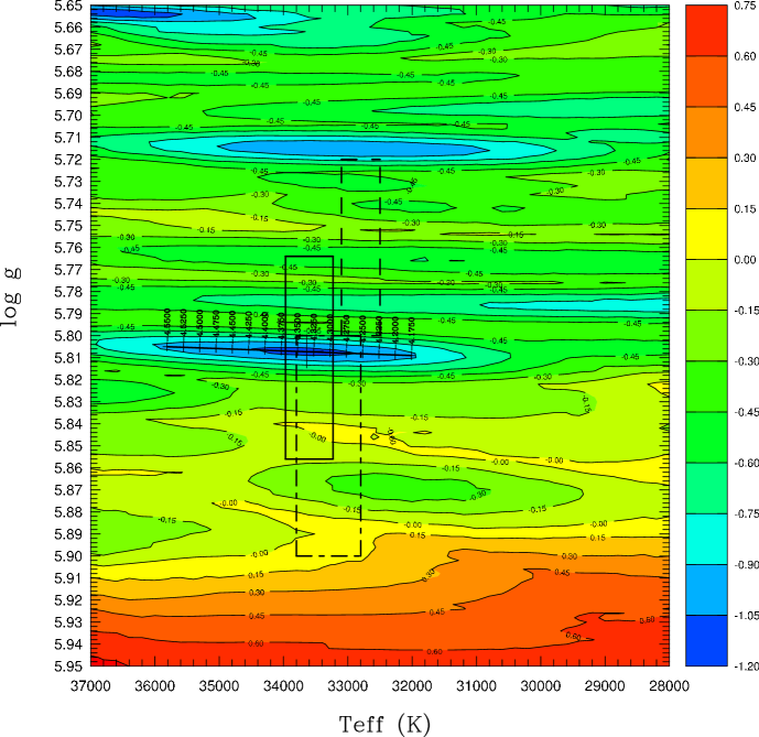
Figure 9: Slice of the “projected” $\overline{\chi}^{2}$-function (in logarithmic units) along the $\log g-T_{{\rm eff}}$ plane at fixed parameter $M_{*}$ set to its optimal value found for the chosen best-fit model solution ($M_{*}=0.4570$ $M_{\odot}$). The projected, $\log q({\rm H})$ parameter was varied between $-2.0$ and $-5.0$ (by steps of 0.025). The labelled axis positioned along the valley of minimum $\overline{\chi}^{2}$ indicates the exact location of the local minimum of $\overline{\chi}^{2}$ for the value of $\log q({\rm H})$ discussed in the text. The solid-line rectangle shows our spectroscopic estimate with its uncertainties for the atmospheric parameters of PG~1219+534, while the dashed-line and dashed-dotted-line rectangles represent the Koen et al. (1999) and Heber et al. (2000; from NLTE H+He model atmospheres) spectroscopic measurements, respectively.

First, there is a small correlation between the $\log q({\rm H})$ and $T_{{\rm eff}}$ parameters. Starting from the derived best-fitting model, changing the value of $\log q({\rm H})$ while keeping $M_{*}$ constant and set to its optimal value generates, in the $\log g-T_{{\rm eff}}$ plane, a shift of the position of the local minimum which mainly follows the effective temperature axis (a tiny shift also occurs in $\log g$). This trend is illustrated with the map provided in Figure 9, which shows the “projection” of the $\log q({\rm H})$ axis onto the surface gravity-effective temperature plane. More precisely, the value associated with each grid point shown on this map is the minimum value found among all the values of the $\overline{\chi}^{2}$-function computed at fixed $T_{{\rm eff}}$, $\log g$ (set to the values associated with the considered grid point), and $M_{*}$ (set to its optimal value, that is $M_{*}=0.4570$ $M_{\odot}$) but with the parameter $\log q({\rm H})$ varying within the limits of the specified search domain, i.e., between $\log q({\rm H)=-5.0}$ and $-2.0$. The various families of solutions identified previously now appear simultaneously as (blue) parallel valleys of low $\overline{\chi}^{2}$ in the $\log g$-$T_{{\rm eff}}$ plane. These correspond, however, to a different range of values for the parameter $\log q({\rm H})$. The small labelled axis positioned along the valley associated with the preferred solution indicates the position of the local minimum of $\overline{\chi}^{2}$ as a function of $\log q({\rm H})$. There is a clear, monotonic trend showing that this minimum shifts from higher effective temperatures (e.g., $T_{{\rm eff}}\sim$ 35,800 K for $\log q({\rm H})\sim-4.55$) to lower $T_{{\rm eff}}$ ($\sim$ 32,000 K for $\log q({\rm H)\sim-4.175}$) as the envelope mass of the star increases (i.e., $\log q({\rm H})$ increases). However, at the same time, we note a degradation of the quality of the period fit (i.e., an increase of the absolute value of $\overline{\chi}^{2}$ associated with the minimum) for values of $\log q({\rm H})$ that departs from the optimal value uncovered. This indicates that the degeneracy associated with the parameter $\log q({\rm H})$ has boundaries, i.e, the optimal solution still occupies the center of a well defined region of the parameter space. Interestingly, we note at this point that best-fit model candidates for the observed periods of PG~1219+534 do all correspond to models with thin H-rich envelopes. In our search, no acceptable asteroseismological fit has been found for models with thick envelopes, i.e., with high values of the parameter $\log q({\rm H})$.

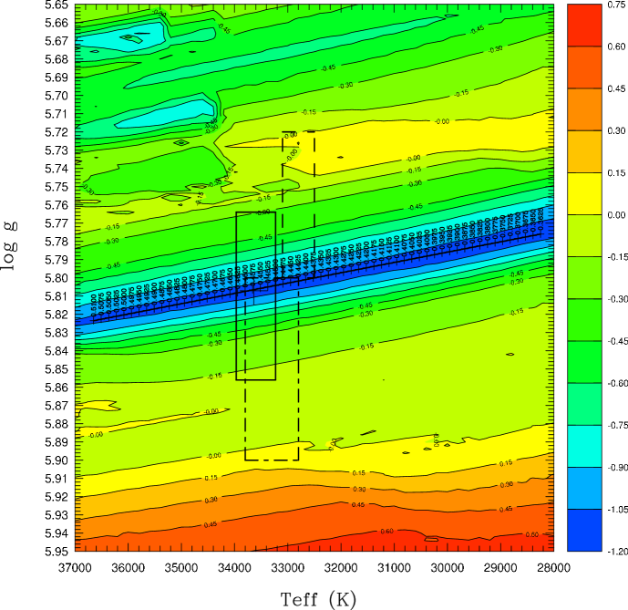
Figure 10: Slice of the “projected” $\overline{\chi}^{2}$-function (in logarithmic units) along the $\log g-T_{{\rm eff}}$ plane at fixed parameter $\log q({\rm H})$ set to its optimal value found for the chosen best-fit model solution ($\log q({\rm H})=-4.3448$). The projected, $M_{*}$ parameter was varied between $0.30$ $M_{\odot}$ and $0.53$ $M_{\odot}$ (by steps of 0.0025 $M_{\odot}$). The labelled axis positioned along the valley of minimum $\overline{\chi}^{2}$ indicates the exact location of the local minimum of $\overline{\chi}^{2}$ for the value of $M_{*}$ discussed in the text. The solid-line rectangle shows our spectroscopic estimate with its uncertainties for the atmospheric parameters of PG~1219+534, while the dashed-line and dashed-dotted-line rectangles represent the Koen et al. (1999) and Heber et al. (2000; from NLTE H+He model atmospheres) spectroscopic measurements, respectively.

A similar map was constructed to visualize the “projection” of the $M_{*}$-axis onto the $\log g-T_{{\rm eff}}$ plane. It is shown in Figure 10. The parameter $\log q({\rm H})$ was kept constant (set to its optimal value of $\log q({\rm H})=-4.3448$) and the total mass was varied within the limits we have defined for the search domain, i.e., between $M_{*}=0.53$ $M_{\odot}$ and $M_{*}=0.30$ $M_{\odot}$. The map indicates clearly that a correlation also exists between the parameter $M_{*}$ and the parameters $T_{{\rm eff}}$ and, to a lesser extent, $\log g$. A change in $M_{*}$ generates a shift in both $T_{{\rm eff}}$ and $\log g$ of the position of the $\overline{\chi}^{2}$ minimum. However, contrary to the case of the $\log q({\rm H})$ parameter discussed previously, we observe no degradation of the quality of the period fit over the entire range considered for the $M_{*}$ parameter. Clearly in the case of PG~1219+534, the impact of changing the value of $M_{*}$ on the theoretical modes fitted to the observed periods can be completely compensated by an adequate change of both $T_{{\rm eff}}$ and $\log g$. This leads to a line-degeneracy in the $\overline{\chi}^{2}$-function along which models provide comparable best-fit solutions of the periods. This is well illustrated in Figure 10 by the presence of a long and flat valley of minimum value of $\overline{\chi}^{2}$ with no high-$T_{{\rm eff}}$ and low-$T_{{\rm eff}}$ boundaries. We also mention that a similar line-degeneracy associated with the second family of solutions, near $\log g\sim 5.71$, does exist, although it is not apparent in Figure 10 as it requires a larger optimal value for the $\log q({\rm H})$ parameter. The labelled axis plotted along the valley of minimum $\overline{\chi}^{2}$ indicates the position of the best-fit solution in the $\log g-T_{{\rm eff}}$ plane for the given value of the total mass. The correlation between $M_{*}$ and ($T_{{\rm eff}}$, $\log g$) is monotonic, as the effective temperature and surface gravity of the solution decreases when the total mass decreases. For instance, a value of $M_{*}=0.5075$ $M_{\odot}$ places the minimum of $\overline{\chi}^{2}$ near $T_{{\rm eff}}\sim$ 36,600 K and $\log g\sim 5.822$, while a value of $M_{*}=0.3650$ $M_{\odot}$ places it near $T_{{\rm eff}}\sim$ 28,400 K and $\log g\sim 5.796$. Note that the correlation with the effective temperature is much stronger than the correlation with the surface gravity parameter. Of course, this trend extends beyond the limits provided in Figure 10, and models with lower (higher) masses lead to even cooler (hotter) solutions. Again, one cannot discriminate between the models on the basis of their $\overline{\chi}^{2}$-value alone, and spectroscopy must be used to lift the degeneracy. The effective temperature derived from the analysis of our medium-resolution, high signal-to-noise MMT spectrum (the solid-line rectangle in Figure 10) allows us to select the appropriate section along the line of degeneracy which corresponds to the “correct” solution. Of course, the necessity to rely on the spectroscopic measurement of $T_{{\rm eff}}$ to uniquely derive the total mass of PG~1219+534 from asteroseismological means indicates, unfortunately, that $M_{*}$ cannot be measured independently of $T_{{\rm eff}}$ for that star. Since, the optimal model first isolated by our GA code with parameters $T_{{\rm eff}}=$ 33,640 K, $\log g=5.8071$, $\log q({\rm H})=-4.3448$, and $M_{*}=0.4570$ $M_{\odot}$ is consistent with the spectroscopic determination of the effective temperature of PG~1219+534, we therefore adopt it as our preferred solution that best matches the period spectrum observed in this star.

Table 4: Pulsation Properties of the Best-Fit Model Solution and Mode Identification.

		$P_{{\rm obs}}$	$P_{{\rm th}}$	$\sigma_{I}$	Stability	$\log E$	$C_{kl}$	$\Delta P/P$	Comments
$\ell$	$k$	(s)	(s)	(rad/s)		(erg)		(%)
0	6	…	76.154	$+5.530\times 10^{-6}$	stable	39.984	…	…
0	5	…	85.013	$-5.270\times 10^{-5}$	unstable	40.028	…	…
0	4	…	98.416	$-4.276\times 10^{-5}$	unstable	40.389	…	…
0	3	…	107.574	$-1.974\times 10^{-5}$	unstable	40.743	…	…
0	2	129.099	129.406	$-8.392\times 10^{-6}$	unstable	41.003	…	$-0.24$	$f_{6}$
0	1	148.775	148.579	$-4.386\times 10^{-7}$	unstable	42.055	…	$+0.13$	$f_{4}$
0	0	…	165.145	$-2.578\times 10^{-7}$	unstable	42.063	…	…
1	7	…	74.783	$+1.932\times 10^{-5}$	stable	39.894	0.0071	…
1	6	…	84.243	$-5.145\times 10^{-5}$	unstable	39.999	0.0067	…
1	5	…	96.410	$-3.634\times 10^{-5}$	unstable	40.434	0.0125	…
1	4	…	105.468	$-2.941\times 10^{-5}$	unstable	40.572	0.0120	…
1	3	128.077	128.176	$-8.586\times 10^{-6}$	unstable	40.999	0.0141	$-0.08$	$f_{1}$
1	2	143.649	143.327	$-8.108\times 10^{-7}$	unstable	41.846	0.0280	$+0.22$	$f_{2}$
1	1	…	164.511	$-2.909\times 10^{-7}$	unstable	42.018	0.0176	…
2	7	…	73.101	$+4.804\times 10^{-5}$	stable	39.746	0.0083	…
2	6	[82.261]	83.016	$-4.504\times 10^{-5}$	unstable	39.981	0.0095	$[-0.92]$	$[f_{10}]$
2	5	…	92.659	$-3.111\times 10^{-5}$	unstable	40.445	0.0223	…
2	4	…	103.257	$-4.166\times 10^{-5}$	unstable	40.420	0.0145	…
2	3	122.408	124.141	$-7.354\times 10^{-6}$	unstable	41.081	0.0413	$-1.42$	$f_{5}$
2	2	135.160	135.309	$-3.273\times 10^{-6}$	unstable	41.331	0.0462	$-0.11$	$f_{8}$
2	1	…	163.248	$-3.474\times 10^{-7}$	unstable	41.953	0.0237	…
2	0	…	196.428	$-3.626\times 10^{-11}$	unstable	44.808	0.4159	…
3	7	…	71.517	$+9.095\times 10^{-5}$	stable	39.612	0.0713	…
3	6	…	80.835	$-2.714\times 10^{-5}$	unstable	40.013	0.0218	…
3	5	…	88.223	$-3.861\times 10^{-5}$	unstable	40.262	0.0310	…
3	4	…	101.203	$-4.846\times 10^{-5}$	unstable	40.348	0.0209	…
3	3	…	115.569	$-7.059\times 10^{-6}$	unstable	41.145	0.0822	…
3	2	133.516	130.982	$-6.919\times 10^{-6}$	unstable	41.059	0.0317	$+1.90$	$f_{3}$
3	1	158.789	160.146	$-4.134\times 10^{-7}$	unstable	41.910	0.0678	$-0.85$	$f_{9}$
3	0	172.214	171.664	$-2.565\times 10^{-8}$	unstable	42.888	0.1774	$+0.32$	$f_{7}$

Of interest in the context of binary evolution scenarios to form hot B subdwarf stars, we find that the low-mass (high-mass) models consistent with the observed periods of PG~1219+534 would require effective temperatures which are significantly cooler (hotter) than currently measured by spectroscopic means. Therefore, those solutions can clearly be rejected on the basis of consistency between spectroscopy and asteroseismology. Remarkably, the mass derived for PG~1219+534, which is compatible with the spectroscopically measured effective temperature, is found to be consistent with the canonical value for Extreme Horizontal Branch objects.

4.4 Period Fit and Mode Identification

The optimal model finally isolated in the previous subsection provides the best simultaneous period match of the nine periods detected in PG~1219+534 and leads to the identification of the pulsation modes involved in the luminosity variations observed in that star. We recall that our global optimization method applied to the asteroseismic analysis of PG~1219+534 does not rely on any previous assumption concerning the values of the degree $\ell$ and the radial order $k$ of the modes being observed. The mode identification appears instead naturally – and somewhat objectively – as a solution (or prediction) of the double-optimization procedure. Details on the derived mode identification and period fit for PG~1219+534 are given in Table 4 (a graphical representation of it is also shown in Figure 11). In addition to the quantities that reflect the properties of the nonradial modes computed from the best-fit model (previously described in Subsection 4.2), Table 4 provides the derived distribution of the observed periods ($P_{{\rm obs}}$) as these were matched to the theoretical periods ($P_{{\rm th}}$). Again, this distribution is the one that minimizes $\chi^{2}$, the sum of the squared difference between the observed periods and their assigned theoretical periods for that model. The relative difference in period $\Delta P/P$ (in %) for each pair ($P_{{\rm obs}},P_{{\rm th}}$) is also given in this table.

We find that the simultaneous fit of the nine periods of PG~1219+534 obtained with the optimal model retained is excellent by current standards. The average relative dispersion between the fitted periods is $\overline{\Delta P/P}\sim 0.6\%$ and the worst difference is less than $\sim 2\%$. On an absolute scale, the average dispersion between the periods is less than $\sim 0.8$ s. This accurate and simultaneous fit of nine periods constitutes, by itself, a remarkable result in the field of asteroseismology. It is comparable in quality (and even slightly better due, in part, to the improved tools used to isolate the optimal model) to the results achieved by Brassard et al. (2001) for the star PG 0014+067. Yet, we emphasize the fact that the accuracy at which the observed periods are measured is approximately one order of magnitude better than the mean period dispersion achieved by our optimal fit. This suggests that, as good as this fit appears to be by current standards of asteroseismology, our equilibrium models describing the structure of sdB stars still suffer from imperfections that leave significant room for improvement, on an absolute scale, in reproducing the current observations. This is, of course, one of the goals to pursue in future asteroseismic studies of sdB pulsators. Interestingly, the marginal detection of an independent period at $82.261$ s ($f_{10}$, shown within brackets in Table 4), although it was not used at all to constrain the search for the optimal model, can indeed, after the fact, be associated with a theoretical mode without degrading the overall quality of the period fit. This result indicates that this period may actually correspond to a real mode excited at very low amplitude in PG~1219+534. In addition, we find that the 9 observed periods (10, if we consider $f_{10}$ as real) all fall within the predicted band of instability, as it is clearly apparent in Table 4. Hence, the model solution derived from our global optimization procedure is also remarkably consistent with the prediction of nonadiabatic pulsation theory applied to our second-generation models of pulsating hot B subdwarfs. The observed periods are identified with radial ($\ell=0$) and nonradial ($\ell=1,$ 2, and 3) $f$- and $p$-modes with radial orders between $k=0-3$ (note that the 82.261 s period, if real, would correspond to a mode with $k=6$, i.e., at the short-period end of the band of instability). Interestingly, the mode identification inferred from the optimal model presented in Table 4 remains unchanged along the line of degeneracy identified in the previous subsection. Thus, the models found along this line of degeneracy can indeed be considered as members of a family of solutions in this respect. Also of interest, we find that the mode identification associated with the second (rejected) family of solutions found near $\log g\sim 5.71$ is similar to the identification proposed, except that all modes are shifted by $\Delta k=+1$. This suggests a periodic behavior, with a third family of acceptable best-fit solutions with modes now shifted by $\Delta k=+2$. However, such a solution would correspond to a model with a surface gravity lower than our bound of $\log g=5.65$ in our search volume in the parameter space, a value in clear conflict with available spectroscopic estimates.

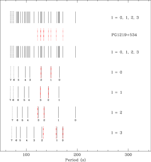
Figure 11: Comparison of the observed period spectrum of PG~1219+534 (thick dashed-dotted-line red segments) with the theoretical pulsation spectrum of the optimal model. For the latter spectrum, solid-line segments indicate excited modes, while dotted-line segments correspond to damped modes. All pulsation modes with $\ell=0$, 1, 2, and 3 in the period interval $70-200$ s are illustrated. The values of the radial order index $k$ are also indicated for each mode. These modes are all acoustic waves (including the $f$-modes). The $g$-modes have periods that fall outside the range of interest for PG~1219+534.

Obviously, from Table 4 and Figure 11, modes of degree up to $\ell=3$ are required in order to account for the mode density observed in PG~1219+534. Moreover, all the observed modes tend to cluster near the low radial order (low-$k$) boundary of the predicted band of instability. Similar mode distributions are actually seen in PG 0014+067 (see Brassard et al. 2001) and in a few other well studied EC14026 pulsators. Often, however, a few periods may be found which correspond to modes positioned near the high-$k$ boundary of the instability band, thus leaving holes of predicted but unseen modes in the period spectrum. A suggestion is that, within the band of excited periods, energy powering up the pulsations may be preferentially distributed among the modes of low radial order. These modes would then reach observable amplitudes more easily, and therefore would be preferentially seen in the light curves of EC14026 pulsators. We also note that we find no strongly established hierarchy of the mode amplitude as a function of $\ell$ for the nine modes identified in Table 4. One would naively expect, at least statistically, some trend of amplitude attenuation when $\ell$ increases, due to geometric cancellation effects. In this context, we note that three of the four dominant periods are indeed associated with modes of degree $\ell=0$ and 1, while periods of lower amplitudes seem to be preferentially associated with modes of degree $\ell=2$ and 3 (with the noticeable exception of the mode $f_{3}$ identified as a $\ell=3$ mode). All these issues related to mode amplitudes are, however, beyond the realm of linear theory and only a nonlinear approach to the pulsation phenomenon will be able to address properly these questions. In the meantime, a purely observational approach, such as searching for the “missing” modes at still higher sensitivity than we could reach with the CFHT, for example using one nigth of Gemini time, could go a long way toward solving this puzzle.

Finally, we stress that the $(k,\ell)$ values attributed to the periods observed in PG~1219+534 constitute a prediction of our seismic analysis which is amenable to independent observational tests. A promising avenue for independent mode identification resides in multicolor photometry (as opposed to one color, “white light” photometry used, for instance, in this study). It is well known from stellar pulsation theory that the apparent amplitude of a nonradial oscillation mode is a function of wavelength. Moreover, how this amplitude changes with wavelength depends on the degree $\ell$ of the mode. Consequently, measuring relative amplitude ratios of modes observed at different wavelength allows, in principle, the identification of their degree $\ell$. Such independent evaluations of the geometry of the modes would obviously provide important tests of our seismic analyses. Some very encouraging results based on that technique have been presented recently by Jeffery et al. (2004), including the suggested identification of a mode with $\ell=4$ in the hot pulsating sdB star KPD 2109+4401.

4.5 Structural Parameters of PG~1219+534

The model that has been isolated and which best represents the observed properties of PG~1219+534, from both the spectroscopy and asteroseismology standpoints, leads to the determination of the fundamental parameters that define the structure of this hot pulsating B subdwarf. A first set of primary quantities corresponding to the main model parameters is naturally derived from this exercise. These primary parameters are the effective temperature $T_{{\rm eff}}$, the logarithm of the surface gravity $\log g$, the total mass $M_{*}$, and the mass of the hydrogen-rich envelope through the quantity $\log q({\rm H})\simeq\log(M_{{\rm env}}/M_{*})$. A set of secondary parameters then follows from the values obtained for the primary quantities. These secondary parameters are the radius $R$ (as a function of $M_{*}$ and $g$), the luminosity $L$ (as a function of $T_{{\rm eff}}$ and $R$), the absolute magnitude $M_{V}$ (as a function of $g$, $T_{{\rm eff}}$, and $M_{*}$ in conjunction with the use of detailed model atmospheres), the distance from Earth $d$ (as a function of $V$ and $M_{V}$). Limits on the rotation period $P_{{\rm rot}}$, equatorial rotation velocity $V_{{\rm eq}}$(as a function of $R$ and $P_{{\rm rot}}$), and projected equatorial rotation velocity $V_{{\rm eq}}\sin i$ could also be set due to the absence of fine structure in the frequency spectrum of PG~1219+534, as multiplets may just be unresolved with the time baseline provided by our observations. The values and limits derived for all these quantities are summarized in Table 5.

Table 5: Inferred Properties of PG~1219+534 ($V=13.24\pm 0.20$).

Quantity	Asteroseismology	Spectroscopy
$\log g$	$5.8071\pm 0.0057$ (0.10%)	$5.810\pm 0.046$ (0.79%)
$T_{\rm eff}$ (K)	33,640 $\pm$ 1,360 (4.04%)	33,600 $\pm$ 370 (1.10 %)
$M_{*}/M_{\odot}$	$0.457\pm 0.012$ (2.63%)	…
$\log(M_{{\rm env}}/M_{*})$	$-4.254\pm 0.147$ (3.46%)	…
$R/R_{\odot}$($M_{*}$, $g$)	$0.1397\pm 0.0028$ (2.00%)	…
$L/L_{\odot}$($T_{\rm eff}$, $R$)	$22.12\pm 4.46$ (20.2%)	$22.01\pm 1.85$ (8.41%)
$M_{V}(\textrm{$g$, $T_{\rm eff}$, $M_{*}$)}$	$4.61\pm 0.12$ (2.60%)	$4.62\pm 0.06$ (1.30%)
$d$($V$, $M_{V}$) (pc)	$532\pm 37$ (6.95%)	$531\pm 23$ (4.33%)
$P_{{\rm rot}}$ (day)	$\gtrsim 3.4$	…
$V_{{\rm eq}}$($R$, $P_{{\rm rot}}$) (km.s-1)	$\lesssim 2.1$	…
$V_{{\rm eq}}\sin i$ (km.s-1)	$\lesssim 2.1$	$\lesssim 10$

An essential ingredient of our asteroseismic study is an evaluation of the uncertainties associated with the parameters derived for the optimal model. The determination of these uncertainties is closely linked to the behavior of the $\overline{\chi}^{2}$ hypersurface in the vicinity of the best-fit solution (see Figures 7 and 8). Following Brassard et al. (2001), we can model the 4-dimensional $\overline{\chi}^{2}$-function in terms of a quadratic expansion considering that the first-order derivatives vanishe at the minimum and that the cross-terms in the second-order derivatives also vanish, in a first approximation, if we consider the four parameters involved to be independent. Clearly, that latter statement is not exact, especially in light of the nature of the degeneracies that have been uncovered in our search for the best-fit solution. These complications will be further discussed below, but we will show that they do not, however, significantly affect the evaluation of the uncertainties associated with the parameters. This simplified approach leads to the following relationship between the variation $\Delta\overline{\chi}^{2}$ and the uncertainties, $\Delta a_{i}$, on the parameters $a_{i}$ (where $a_{1}=\log g$, $a_{2}=T_{{\rm eff}}$, $a_{3}=M_{*}$, and $a_{4}=\log q[{\rm H}]$)

$$\Delta\overline{\chi}^{2}=\sum_{i=1}^{4}\frac{1}{2}\frac{\partial^{2}\overline{\chi}^{2}}{\partial a_{i}^{2}}\bigg{|}_{{\rm min}}(\Delta a_{i})^{2}\,\,\,\,.$$ (2)

The second-order derivatives are evaluated at the position of the optimal model and are estimated on the basis of the $\overline{\chi}^{2}$-values found in the grids specifically constructed around this optimal model (again, shown in Figures 7 and 8). In order to obtain a conservative estimate of the uncertainty on a given parameter, we assume that the variation $\Delta\overline{\chi}^{2}$ is due exclusively to the variation of that one parameter, thus leading to the relationship

$$\Delta a_{i}=\sqrt{2\Delta\overline{\chi}^{2}\bigg{/}\frac{\partial^{2}\overline{\chi}^{2}}{\partial a_{i}^{2}}\bigg{|}_{{\rm min}}}\,\,\,\,.$$ (3)

The problem now resides in evaluating the quantity $\Delta\overline{\chi}^{2}$. The merit function $\overline{\chi}^{2}$ that we have defined to measure the quality of the period fit is not a standard $\chi_{{\rm std}}^{2}$ for which usual formulae can apply to estimate the normal errors. A renormalization of this function is needed and can be achieved following the prescription of Press et al. (1985; see also Bevington 1969) assuming that we have obtained a perfect fit of the observations. In that case, the standard $\chi_{std}^{2}$ at the minimum is equal to the number of degrees of freedom $\nu$, here equal to 5 (9 periods minus four free parameters). This leads to a scale factor $S$ between the standard minimum $\chi_{{\rm std}}^{2}$ and the value of the merit function $\overline{\chi}^{2}$ at the optimal point in parameter space given by $S=5/0.0784=63.7755$. We next compute the value of $\Delta\chi_{{\rm std}}^{2}$ that must be added to $\chi_{{\rm std}}^{2}$ to cover a range of parameter space sufficient to reach a given confidence level in the estimates of the uncertainties on the parameters. We adopt the $1\sigma$ limit (68.3% confidence level) and compute $\Delta\chi_{{\rm std}}^{2}$ using the Gammq routine of Press et al. (1985) for the truncated gamma function. For the case $\nu=5$, we find that $\Delta\chi_{{\rm std}}^{2}=5.8907$. Applying the renormalization according to the scale factor $S$, this corresponds to $\Delta\overline{\chi}^{2}=0.0924$, the value we now use in equation (3). We finally find that, at the 68.3% confidence level, the error estimates associated with the four primary parameters of PG~1219+534 (i.e., $\log g$, $T_{{\rm eff}}$, $M_{*}$, and $\log[M_{{\rm env}}/M_{*}]\simeq\log q[{\rm H}]$) correspond to the values given in Table 5. These error estimates are also illustrated as dotted-line rectangles on the maps provided in Figures 7 and 8. Uncertainties on the secondary quantities are then easily derived from the values obtained for the primary parameters.

As mentioned in the previous paragraph, this approach relies in part on the assumption that the parameters are independent, an assumption that is not well verified in practice due, in particular, to the degeneracy in parameter space of the optimal model solution. To deal with such a difficulty, one could consider, as an alternative method to provide estimates of the uncertainties, the relatively strong constraint brought by spectroscopy on the determination of the effective temperature. Using projection maps of the merit function such as those illustrated in Figures 9 and 10, one can delimit the domain of acceptable values for all model parameters according to the limits (i.e., the evaluated errors) imposed by spectroscopy on the $T_{{\rm eff}}$ values. A close examination of these maps indicates, however, that the uncertainties derived from this approach are of the same order as the values computed from the method introduced by Brassard et al. (2001). We therefore maintain our first evaluation of the errors given in Table 5 as representative of the $1\sigma$ uncertainties associated with the derived fundamental parameters of PG~1219+534.

These asteroseismic results deserve additional comments as they are representative of the current potential and limitations of asteroseismology applied to EC14026 pulsators. A first significant contribution of asteroseismology to the study of sdB stars is the ability to derive values for the surface gravity $\log g$ with unprecedented accuracy, i.e., improved by a factor of $\sim 10$ compared to current spectroscopic measurements, typically. This reflects the fact that the $p$-mode periods are particularly sensitive to the gas density which strongly affects the speed at which acoustic waves propagate in the stellar interior (i.e, the sound speed). And how dense and compact a sdB star is largely depends on the $\log g$ parameter (see, e.g., Charpinet et al. 2002). On the other hand, we find that the asteroseismic value derived for the effective temperature is not well constrained, due in part to the fact that the $p$-mode periods are relatively insensitive to this parameter in sdB stars, but also because solution degeneracies may prevent from uniquely measuring that quantity through asteroseismology only. Notably, spectroscopy turns out to be a much more accurate method to measure $T_{{\rm eff}}$ and allows to lift eventual degeneracies in the asteroseismic solutions. Therefore, we stress that both methods have indeed complementary roles to play in this respect. In addition to those “classical” parameters, asteroseismology allows for the determinations at an interesting level of accuracy of fundamental structural quantities, such as the total mass and the thickness of the outer H-rich envelope in hot B subdwarfs, two key parameters for testing theories of formation and evolution of stars on the Extreme Horizontal Branch. These two quantities cannot generally be determined otherwise, except for some masses of sdB stars known through the study of binary systems containing an sdB component, but with a relatively poor accuracy on the derived value. For its part, the determination of the mass of the outer H-rich envelope is a pure product of asteroseismology and, beside theory, this quantity cannot be constrained by other known means. Determinations of $M_{{\rm env}}/M_{*}$ for other EC14026 pulsators through our seismic approach may provide, in the future, interesting insight into the internal structure and evolution of these old extreme horizontal branch stars.

To conclude this subsection, we point out that we are fully aware that our asteroseismic determinations of the global parameters of PG~1219+534 are only as good, in an absolute sense, as the constitutive physics that went into the construction of the equilibrium models. Future improvements in our ability to understand and model sdB stars at the level of the microphysics (i.e., the equation of state, the opacity, the radiative levitation, initial conditions, and so on) will necessarily lead to revised estimates of these parameters and, hopefully, to improved matches of the observed periods. Nevertheless, we do point out that solid credibility must already be given to current available constitutive physics since, after successfully reproducing the 13 observed pulsation periods of PG 0014+067 to better than $\sim 0.8$% (Brassard et al., 2001), the current models are also able to explain the presence of 9 pulsation periods in the EC 14026 star PG~1219+534 with an average accuracy of $\sim 0.6$% on the periods.

5 Summary and Conclusion

We observed the luminosity variations of the relatively bright ($V=13.24\pm 0.20$), rapidly pulsating hot B subdwarf PG 1219+534 at high sensitivity at the CFHT during a dedicated run in 2004, March. Such observations were part of an ongoing, long-term project to monitor the pulsations of EC14026 stars at sufficiently high S/N ratios to allow for the detection of low-amplitude modes. The objective is to increase the number of detected modes in known EC14026 stars, as it constitutes a necessary step for ultimately applying asteroseismic methods to probe the inner structure of these objects. Our past observing experience have shown that the “marriage” between the Montréal 3-channel photometer Lapoune and the CFHT is particularly efficient for this purpose. For several sdB pulsators observed so far in the course of this program, we could typically double the number of mode detections compared to existent data from other sites (see, Charpinet 2001). Our most recent observations along this line made no exception to the rule and led to the clear identification of nine independent oscillation periods in PG~1219+534. This constitutes a significant improvement over the original data available for this star, which allowed for the detection of only four dominant periods (Koen et al., 1999).

From the time series analysis using standard methods that combine Fourier analysis, least squares fits of the light curve, and prewhitening methods, we found that PG~1219+534 has a relatively simple pulsation spectrum characterized by well separated components easily recognizable as independent modes. Moreover, we found no indication of close frequency structures (such as multiplets), at least at the frequency resolution achieved during these observations ($\sim 3.44$ $\mu$Hz). This indicates that PG~1219+534 is likely a slow rotator, with a lower limit on its rotation period that can be set to $\sim 3.4$ days (i.e., the time baseline of our observing run). The contrast is sharp with two other members of the EC14026 class, PG 1605+072 (Koen et al., 1998) and KPD 1930+2752 (Billères et al., 2000), which are rather exceptional in that both show very complex oscillation spectra due most certainly to rapid rotation. PG~1219+534 appears instead as a well behaved sdB pulsator with a rich – yet simple enough – period spectrum ideally suited for detailed asteroseismology. Interestingly, we found that, for this particular star, one single night of excellent CFHT data turned out to have all the seismic information necessary for a subsequent successful asteroseismological exercise. Our detailed analysis of the light curves of PG~1219+534 also illustrated the fact that, for EC 14026 pulsators having an easily resolved period spectrum, the search for a better signal-to-noise ratio is of higher interest for the sake of asteroseismology than a longer time baseline and/or coverage. Indeed, we showed that mixing high quality light curves with low S/N ratio data (due to degraded observing conditions) can basically ruin all the benefit of having the high sensitivity data, since the overall noise level in the Fourier domain will be dominated by the noise introduced by the worst time series included. This has, of course, implications on how one should treat heterogeneous data sets such as those gathered during multisite campaigns, for instance. We mention, along this line, that the best asteroseismic return for more complex EC14026 pulsators that need multisite contiguous coverage to unambiguously resolve their pulsation spectrum would require the acquisition of high sensitivity photometric data which is as homogeneous as possible in quality. In this context, we are engaged in the organisations of bi- (or tri-) site campaigns that would involve 4m-class telescopes positioned at strategic longitudes. Our efforts are presently directed toward a joint utilisation of the CFHT with Lapoune and the WHT with Ultracam as both telescopes are ideally located geographically and would provide an almost complete coverage. This, of course, would be in addition to recent efforts to perform multicolor fast photometry (Jeffery et al., 2004) and time resolved spectroscopy (O’Toole et al., 2004) on these pulsating stars.

Based on the nine oscillation periods identified in the light curve of PG~1219+534, we have attempted a detailed asteroseismic analysis of this EC14026 star. Our approach relied on the well-known forward method with the goal of finding objectively the model that would best match the set of periods observed in this star with a set of theoretical periods. We have used the second generation sdB models of Charpinet et al. (1997) to compute the theoretical periods since those have proved to account quite well for the class properties of the EC14026 pulsators (Charpinet et al., 2001). Due to the lack of mode identification from the available “white light” photometric data, we performed a double-optimization procedure that takes place simultaneously at the period matching level and in the model parameter space, leading objectively to the best fit of the asteroseismic observations. In the present study, we have used the Toulouse package of numerical tools specifically developed, over the years, for the purpose of asteroseismology and which includes a genetic algorithm based period matching code (dedicated to the first optimization step), a parallel genetic algorithm based code, and a parallel grid computing code allowing for an efficient exploration of the vast parameter space (the second optimization step).

Our thorough exploration of parameter space led us to first isolate two families of model solutions that equally best-match the observed periods of PG~1219+534. These families of models have surface gravities around $\log g\sim 5.81$ and $\log g\sim 5.71$, respectively, and correspond to slightly different mode identifications. This degeneracy in the asteroseismic solution could not be lifted solely on the basis of period fit quality, and additional constraints were required to select the “correct” one. Such constraints were provided by the available spectroscopic measurements for the atmospheric parameters of PG~1219+534. An ongoing project aimed at improving the spectroscopic characterization of sdB stars (including both the rapid and slow pulsators), and which is based on the acquisition of high resolution, high S/N ratio spectra with the blue spectrograph at the new MMT, has proved essential in this context. The independently derived atmospheric parameters for PG~1219+534, $T_{{\rm eff}}=$ 33,600 $\pm$ 370 K and $\log g=5.810\pm 0.046$, allowed us to clearly reject the family of model solutions found at low surface gravity (i.e., near $\log g\sim 5.71$). Concentrating on the preferred solution located near $\log g\sim 5.81$, we found however that another kind of degeneracy exists in the solution which, again, precludes from uniquely isolate an optimal model from asteroseismology alone. This problem occurs due to concurrent effects of model parameters on the pulsation periods, leading, in the worst case, to a line-degeneracy of the best-fit solutions that mostly link the total mass parameter with the effective temperature parameter. We found, indeed, that seismic solutions of comparable quality exist for all values of the total mass of the star, but these solutions have values for $T_{{\rm eff}}$ that are correlated. The trend uncovered is monotonic and indicates that optimal models of low-mass (down to $0.30$ $M_{\odot}$) require cooler effective temperatures, while optimal models of high-mass (up to $0.53$ $M_{\odot}$, but also verified with a few additional calculations at higher masses) need hotter effective temperatures. It is again spectroscopy that provided the additional information needed to bypass this difficulty, as using the well-constrained value of $T_{{\rm eff}}$ derived from this method led to the determination of a unique viable optimal model solution that fit consistently PG~1219+534, both asteroseismologically and spectroscopically.

The basic properties of PG~1219+534 as inferred from our combined spectroscopic and asteroseismic approach have been summarized in Table 5. The quest for an optimal seismic model of PG~1219+534 has revealed that accurate spectroscopy remains an essential ingredient for detailed asteroseismology of EC 14026 stars in order to converge toward a unique solution. A relatively precise determination of the surface gravity using spectroscopic techniques is generally helpful to discriminate between families of potential seismic solutions. Once the “right” family has been chosen, though, the constraint brought by asteroseismology on the value of $\log g$ is much tighter than the precision that spectroscopy can currently provide. This is one of the outstanding outcomes of asteroseismology as it leads to measurements of the surface gravity of EC 14026 stars at unprecedented accuracy (a gain of a factor $\sim 10$, typically). The opposite is true for the effective temperature and the spectroscopic value for this parameter must clearly be preferred. Moreover, in the case of PG~1219+534, the line degeneracy uncovered for the seismic solution precludes an independent measurement of $T_{{\rm eff}}$ through asteroseismological means.

Another outstanding outcome of asteroseismology is the measurement of the total mass and the mass of the H-rich envelope at an interesting level of accuracy. In our study of PG~1219+534, we found however that the total mass could not be inferred independently of the spectroscopic measurement of the effective temperature. Nonetheless, the value derived, $M=0.457\pm 0.012$ $M_{\odot}$, indicates a mass of PG~1219+534 that is close to the canonical value for sdB stars. Although this value of the mass depends on how reliable the spectroscopic estimate of $T_{{\rm eff}}$ is (particularly in regards to eventual systematic effects), we stress that significantly different masses than the derived – close to canonical – value, such as some scenarios of binary evolution suggest, would require a shift of several thousand Kelvins in effective temperature to be compatible with asteroseismology. Such a drastic change in the evaluation of $T_{{\rm eff}}$ from spectroscopy is highly unlikely and, therefore, we are confident in concluding that PG~1219+534 has a mass close to the canonical mass of extreme horizontal branch stars.

We found that our optimal model solution is able to reproduce simultaneously the 9 periods observed in PG~1219+534 with an average dispersion of only $\sim 0.6$%. The observed periods correspond to low-order $\ell=0$, 1, 2, and 3 acoustic modes that are, indeed, predicted to be excited according to nonadiabatic pulsation theory. It is a remarkable result (not often achieved so far in the field of asteroseismology) that the model solution uncovered for PG 1219+534 can, at the same time, reproduce all the periods observed in this star at a relatively high level of accuracy, be consistent with nonadiabatic theory, and satisfy the spectroscopic constraints. Such a consistency between three independent aspects of the modeling of these pulsating stars is a result that was not guaranteed at the outset. This is strong indication that the basic constitutive physics which enters in the construction of our current models used for the asteroseismic analyses of EC 14026 stars is sound, especially as it follows similar results already obtained for another rapid sdB pulsator, PG 0014+067 (Brassard et al., 2001). Furthermore, the excellent agreement between observations and theory at the nonadiabatic level brings further proof that the iron bump opacity mechanism of Charpinet et al. (1997) is indeed at the origin of the EC 14026 phenomenon.

Finally, we note that the mode identification resulting from our detailed asteroseismic analysis of PG~1219+534 constitutes a prediction that, in principle, can be independently tested using multicolor photometry. Along this line, we initiated a project to use the Far UV Spectroscopic Explorer (FUSE) as a fast-photometer (a possibility offered by the so-called “Time-Tag” mode of the instrument) that would provide a light curve of PG~1219+534 in the FUV (near $\sim 1000$Å) bandpass. Combined with nearly simultaneous ground based observations in the optical, this project should lead to strong independent constraints on the $\ell$ value of the modes seen in PG~1219+534, from which the predicted mode identification reported in this paper will be checked.