Self-Calibration of Cluster Dark Energy Studies: Observable-Mass Distribution

Abstract

The exponential sensitivity of cluster number counts to the properties of the dark energy implies a comparable sensitivity to not only the mean but also the actual distribution of an observable mass proxy given the true cluster mass. For example a $25\%$ scatter in mass can provide a $\sim 50\%$ change in the number counts at $z\sim 2$ for the upcoming SPT survey. Uncertainty in the scatter of this amount would degrade dark energy constraints to uninteresting levels. Given the shape of the actual mass function, the properties of the distribution may be internally monitored by the shape of the observable mass function. An arbitrary evolution of the scatter of a mass-independent Gaussian distribution may be self-calibrated to allow a measurement of the dark energy equation of state of $\sigma(w)\sim 0.1$. External constraints on the mass variance of the distribution that are more accurate than $\Delta\sigma_{\ln M}^{2}<0.01$ at $z\sim 1$ can further improve constraints by up to a factor of 2. More generally, cluster counts and their sample variance measured as a function of the observable provide internal consistency checks on the assumed form of the observable-mass distribution that will protect against misinterpretation of the dark energy constraints.

I Introduction

It is well known that cluster counts as a function of their mass are exponentially sensitive to the amplitude of the linear density field and hence the dark energy dependent growth of structure. Unfortunately the mass of a cluster is not a direct observable and their numbers can only be counted as a function of some observable proxy for mass. Typical proxies include the Sunyaev-Zel’dovich flux decrement, X-ray temperature, X-ray surface brightness or gas mass, optical galaxy richness, and the weak lensing shear. The exponential sensitivity to mass translates into a comparable sensitivity to the whole distribution of the observable given the mass not just the mean relationship.

While scatter in the observable-mass relation is typically addressed in studies of the local cluster abundance (e.g. Ikebe et al. (2002)), it is commonly ignored in forecasts for upcoming high redshift surveys (e.g. Haiman et al. (2001); Hu and Kravtsov (2003); Wang et al. (2004)). While it is true that scatter in the observable of a known form does little to degrade the dark energy information, uncertainties in the distribution directly translate into uncertainties in the dark energy inferences that must be controlled.

In this Paper we undertake a general study of the impact of uncertainty in the observable-mass distribution on high redshift cluster counts. Previous work on forecasting prospects for dark energy constraints have examined the effect of scatter under specific and typically more restrictive assumptions. For example, the change in the number counts, known as Eddington bias Eddington (1913), has been assessed for a fixed cut in signal-to-noise of cluster detection via the Sunyaev-Zel’dovich flux in a hydrodynamic simulation Holder et al. (2000) and through modeling a constant scatter in mass Battye and Weller (2003). However it is the uncertainty in the scatter, or the error in the correction of the bias, that degrades dark energy constraints. Along these lines, Levine et al. Levine et al. (2002) considered the marginalization of a constant scatter in the mass-temperature relation for clusters but with strong external priors on the dark energy parameters.

Prospects for the self-calibration of the mean observable-mass relation have been extensively studied recently. Self-calibration relies on the fact that both the shape of the mass function Hu (2003) and the clustering of clusters Majumdar and Mohr (2003) can be predicted from cosmological simulations. Much of the information in the latter can be extracted from the angular variance of the counts so that costly spectroscopy can be avoided Lima and Hu (2004). Thus by demanding consistency between the counts and their sample variance across the sky as a function of the observable mass, one can jointly solve for the cosmology and the mean observable mass relation. Here we show that the shape of the mass function is even more effective at monitoring the scatter in the observable-mass relation.

We begin in §II with a discussion of our parameterization of the observable-mass distribution and assess its implications for the dark energy. We examine the prospects for self-calibration in §III and conclude in §IV.

II Observable-Mass Distribution

The cosmological utility of cluster number counts arises from their exponential sensitivity to the amplitude of the linear density field. For illustrative purposes, we will employ a fit to simulations for the mass function or the differential comoving density of clusters Jenkins et al. (2001)

$${d\bar{n}\over d\ln M}=0.3{\rho_{m}\over M}{d\ln\sigma^{-1}\over d\ln M}\exp[-|\ln\sigma^{-1}+0.64|^{3.82}]\,,$$ (1)

where $\sigma^{2}(M;z)\equiv\sigma^{2}_{R}(z)$, the linear density field variance in a region enclosing $M=4\pi R^{3}\rho_{m}/3$ at the mean matter density today $\rho_{m}$.

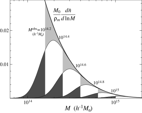
Figure 1: Scatter of $\sigma_{\ln M}=0.25$ in the observable-mass relation changes the mass distribution of clusters above an observable threshold $M^{\rm obs}$ (curves) to provide an excess of clusters scattering up (dark shaded) versus down (light shaded) across the threshold. Here the intrinsic mass function (thick line) has been normalized to $M_{0}=10^{14}h^{-1}M_{\odot}$ and evaluated at $z=0$.

To exploit this exponential sensitivity, the observable-mass distribution must be known to a comparable accuracy. Let us consider the probability of assigning a mass $M^{\rm obs}$ to a cluster of true mass $M$ to be given by a Gaussian distribution in $\ln M$ as motivated by the observed scatter in the scaling relations between typical cluster observables (e.g. Ikebe et al. (2002))

$$p(M^{\rm obs}|M)={1\over\sqrt{2\pi\sigma_{\ln M}^{2}}}\exp\left[-x^{2}(M^{\rm obs})\right]\,,$$ (2)

where

$$x(M^{\rm obs})\equiv{\ln M^{\rm obs}-\ln M-\ln M^{\rm bias}\over\sqrt{2\sigma_{\ln M}^{2}}}\,.$$ (3)

For simplicity we will allow the mass variance $\sigma_{\ln M}^{2}$ and the mass bias $\ln M^{\rm bias}$ to vary with redshift but not mass. We implicitly exclude sources of scatter due to noise in the measurement of $M^{\rm obs}$ which certainly would depend on $M^{\rm obs}$ but in a way that is known given the properties of a specific survey. More generally, our qualitative results will hold so long as any trend in mass at a fixed redshift is known.

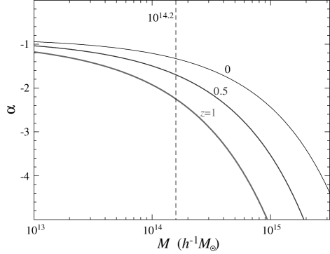
Figure 2: Local power law index $\alpha$ of the mass function as a function of mass $d\bar{n}/d\ln M\propto M^{\alpha}$ for $z=0$, $0.5$ and $1$. The relative importance of scatter versus bias can be scaled through $\alpha$ and Eqn. (9) to alternate mass and redshift ranges than considered here.

The average number density of clusters within a range defined by cuts in the observable mass $M^{\rm obs}_{i}\leq M^{\rm obs}\leq M^{\rm obs}_{i+1}$ is

$$\bar{n}_{i} \equiv\int_{M^{\rm obs}_{i}}^{M^{\rm obs}_{i+1}}{dM^{\rm obs}\over M^{\rm obs}}\int{dM\over M}{d\bar{n}\over d\ln M}p(M^{\rm obs}|M)$$

$$=\int{dM\over M}{d\bar{n}\over d\ln M}{1\over 2}\left[{\rm erfc}(x_{i})-{\rm erfc}(x_{i+1})\right]\,,$$ (4)

where $x_{i}=x(M^{\rm obs}_{i})$. The mean number of clusters in a given volume $V_{i}$ is then

$$\bar{m}_{i}=\bar{n}_{i}V_{i}\,.$$ (5)

Note that in the limit that $\sigma_{\ln M}^{2}\rightarrow 0$ and $M^{\rm obs}_{i+1}\rightarrow\infty$, $\bar{m}_{i}$ is the usual cumulative number counts above some sharp mass threshold.

An unknown scatter or more generally uncertainty in the distribution of the observable mass given the true mass causes ambiguities in the interpretation of number counts. Fig. 1 shows the expected mass distribution of clusters above a certain $M^{\rm obs}$ given a scatter of $\sigma_{\ln M}=0.25$. As the observable threshold reaches the exponential tail of the intrinsic distribution, the excess of upscattered versus downscattered clusters can become a significant fraction of the total. Since at high redshift a fixed $M^{\rm obs}$ will be further on the exponential tail, even a constant but unknown scatter can introduce a trend in redshift that will degrade the dark energy information in the counts.

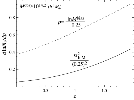
Figure 3: Fractional sensitivity of the number counts in redshift to the mass variance $\sigma_{\ln M}^{2}$ and bias $\ln M^{\rm bias}$ scaled to $(0.25)^{2}$ and $0.25$ respectively. The relative importance of the variance increases with $z$.

The relative importance of scatter can be understood by examining the sensitivity of the counts to the scatter around $\sigma_{\ln M}^{2}=0$

$$\lim_{\sigma_{\ln M}^{2}\rightarrow 0}{\partial\ln\bar{m}_{i}\over\partial\sigma_{\ln M}^{2}}=-{1\over 2\bar{n}_{i}}{d^{2}\bar{n}\over d\ln^{2}M}\Big{|}_{x_{i+1}=0}^{x_{i}=0}\,.$$ (6)

Thus the steepness of the mass function around the thresholds in the observable mass determines the excess due to upscatters. Note that it is the variance $\sigma_{\ln M}^{2}$ rather than the rms scatter $\sigma_{\ln M}$ that controls the upscattering effect. For example, since

$$\lim_{\sigma_{\ln M}^{2}\rightarrow 0}\left[{\partial\ln\bar{m}_{i}\over\partial\sigma_{\ln M}}=2\sigma_{\ln M}{\partial\ln\bar{m}_{i}\over\partial\sigma_{\ln M}^{2}}\right]=0\,,$$ (7)

the sensitivity to the rms scatter depends on the true value of the scatter and vanishes at $\sigma_{\ln M}=0$. Conversely from Eqn. (6), an observable with say half the scatter would have a quarter of the fractional effect on number counts in this limit.

On the other hand the sensitivity to the bias is given by

$$\lim_{\sigma_{\ln M}^{2}\rightarrow 0}{\partial\ln\bar{m}_{i}\over\partial\ln M^{\rm bias}}={1\over\bar{n}_{i}}{d\bar{n}\over d\ln M}\Big{|}_{x_{i+1}=0}^{x_{i}=0}\,.$$ (8)

Thus the relative importance of scatter compared with bias can be estimated through the local power law slope of the mass function $d\bar{n}/d\ln M\propto M^{\alpha}$ (see Fig. 2)

$$-{1\over 2}{{d^{2}\bar{n}/d\ln^{2}M}\over{d\bar{n}/d\ln M}}=-{1\over 2}\alpha(M)\,.$$ (9)

Uncertainties in scatter can dominate those of bias for the steep mass function at high mass or redshift.

These expectations are borne out at finite scatter by a direct computation of the number count sensitivity. Fig. 3, shows the sensitivity of number counts above $M^{\rm obs}=10^{14.2}h^{-1}M_{\odot}$ in redshift bins of $\Delta z=0.1$ evaluated around $\ln M^{\rm bias}=0$ and a finite scatter $\sigma_{\ln M}^{2}=(0.25)^{2}$. Both in terms of absolute sensitivity and relative sensitivity compared to the bias, the importance of scatter increases with redshift. Uncertainties in the mass variance of $\Delta\sigma_{\ln M}^{2}=(0.25)^{2}$ would produce a $\sim 50\%$ uncertainty in the number counts at $z=2$. For the high $z$ counts to provide cosmological information, the scatter must be known to significantly better than this level.

Given that the relative effect of scatter depends on the local slope of the mass function, measuring the counts as a function of $M^{\rm obs}$ monitors the scatter in the mass-observable relation. Combined with additional information in the sample variance of the number counts, an unknown evolution in $M^{\rm bias}$ and $\sigma_{\ln M}^{2}$ may be internally calibrated.

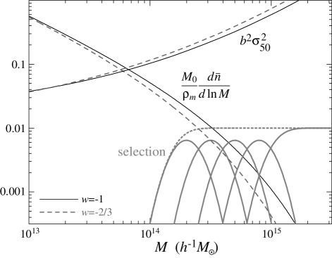
Figure 4: Simulations predict the sample variance of counts, shown for a typical volume ($R=50h^{-1}$ Mpc, upper curves), and the shape of the mass function (lower curves) as a function of mass. Self-calibration is assisted by binning the selection, multiplied here by $0.01$ for clarity and shown here with $\sigma_{\ln M}=0.25$, into 5 bins of $\Delta\log_{10}M^{\rm obs}=0.2$ (solid lines) as opposed to a single threshold binning of $M^{\rm obs}\geq 10^{14.2}h^{-1}M_{\odot}$ (dotted line). With only threshold binning, joint changes to the cosmology, mass bias, and scatter are degenerate with the dark energy equation of state $w$ (long dashed lines).

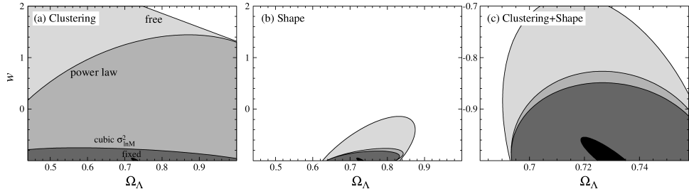
Figure 5: Efficacy of self-calibration through (a) the clustering information in the sample variance alone, (b) the shape of the counts in 5 mass bins and (c) both (note the $\times 10$ change in scale). From outer to inner ellipse, each at the 68% CL, the assumptions on the redshift evolution of the bias and scatter are tightened from a free functional form of 20 parameters each in bins of $\Delta z=0.1$, a power law evolution in $M^{\rm bias}$, an additional cubic form for the evolution in $\sigma_{\ln M}^{2}$. Without any form of self-calibration no relevant dark energy constraints are possible under any of these assumptions. For reference we show the baseline results of a completely fixed $M^{\rm bias}$ and $\sigma_{\ln M}^{2}$ as the solid innermost ellipse

III Self-Calibration

To assess the impact of uncertainties in the observable-mass distribution, we employ the usual Fisher matrix technique. For illustrative purposes we take a fiducial cluster survey with specifications similar to the planned South Pole Telescope (SPT) Survey: an area of 4000 deg² and a sensitivity corresponding to a constant $M^{\rm obs}_{\rm th}=10^{14.2}h^{-1}M_{\odot}$. We further divide the number counts into bins of redshift $\Delta z=0.1$ from an assumed optical photometric followup out to $z=2$ and 400 angular cells of 10 deg² for assessment of the sample variance of the counts (see Lima and Hu (2004) for an exploration of these choices). Finally to study the efficacy of self-calibration from binning of the observable, we compare 5 bins of $\Delta\log_{10}M^{\rm obs}=0.2$ versus a single bin of $M^{\rm obs}\geq M^{\rm obs}_{\rm th}$ (see Fig. 4).

The Fisher matrix is constructed out of predictions for the number counts and their covariance. The mean number counts $m_{i}$ possess a sample covariance of Hu and Kravtsov (2003)

$$S_{ij} = \langle(m_{i}-\bar{m}_{i})(m_{j}-\bar{m}_{j})\rangle$$ (10)

$$= {b_{i}\bar{m}_{i}b_{j}\bar{m}_{j}\over V_{i}V_{j}}\int{d^{3}k\over(2\pi)^{3}}W_{i}^{*}({\bf k})W_{j}({\bf k})P(k)\,,$$

given a linear power spectrum $P(k)$ and the Fourier transform of the selection window $W_{i}({\bf x})$. The pixel index $i$ here runs over unique cells in redshift, angle, and observable mass. Here $b_{i}$ is the average bias of the clusters predicted from the distribution in Eqn. (4)

$$b_{i} ={1\over\bar{n}_{i}}\int{dM\over M}{d\bar{n}_{i}\over d\ln M}b(M;z_{i})\,,$$ (11)

where we take a fit to simulations of Sheth and Tormen (1999)

$$b(M;z)=1+{a_{c}\delta_{c}^{2}/\sigma^{2}-1\over\delta_{c}}+{2p_{c}\over\delta_{c}[1+(a\delta_{c}^{2}/\sigma^{2})^{p}_{c}]}$$ (12)

with $a_{c}=0.75$, $p_{c}=0.3$, and $\delta_{c}=1.69$. That the sample variance, or the clustering of clusters, is a known function of mass provides a second means of self-calibration Majumdar and Mohr (2003). Note that for a given volume defined by the redshift and solid angle, the mean counts for different ranges in the observable mass $M^{\rm obs}$ are fully correlated. Finally the total covariance matrix is the sample covariance plus shot variance

$$C_{ij}=S_{ij}+\bar{m}_{i}\delta_{ij}\,.$$ (13)

The Fisher matrix quantifies the information in the counts on a set of parameters $p_{\alpha}$ as Holder et al. (2001); Lima and Hu (2004)

$$F_{\alpha\beta} = \bar{\bf m}^{t}_{,\alpha}{\bf C}^{-1}\bar{\bf m}_{,\beta}+{1\over 2}{\rm Tr}[{\bf C}^{-1}{\bf S}_{,\alpha}{\bf C}^{-1}{\bf S}_{,\beta}]\,,$$ (14)

where the first piece represents the information from the mean counts and the second piece the information from the sample covariance of the counts. We have here arranged the counts per pixel $i$ into a vector ${\bf m}\equiv(m_{1},\ldots,m_{N_{\rm pix}})$ and correspondingly their covariance into a matrix. The Fisher matrix approximates the covariance matrix of the parameters $C_{\alpha\beta}\approx[{\bf F}^{-1}]_{\alpha\beta}$ such that the marginalized error on a single parameter is $\sigma(p_{\alpha})=[{\bf F}^{-1}]_{\alpha\alpha}^{1/2}$. When considering prior information on parameters of a given $\sigma(p_{\alpha})$ we add to the Fisher matrix a contribution of $\sigma^{-2}(p_{\alpha})\delta_{\alpha\beta}$ before inversion.

For the parameters of the Fisher matrix we begin with six cosmological parameters: the normalization of the initial curvature spectrum $\delta_{\zeta}(=5.07\times 10^{-5})$ at $k=0.05$ Mpc^-1 (see Hu and Jain (2004) for its relationship to the more traditional $\sigma_{8}$ normalization), its tilt $n(=1)$, the baryon density $\Omega_{b}h^{2}(=0.024)$, the dark matter density $\Omega_{m}h^{2}(=0.14)$, and the two dark energy parameters of interest: its density $\Omega_{\rm DE}(=0.73)$ relative to critical and equation of state $w(=-1)$ which we assume to be constant. Values in the fiducial cosmology are given in parentheses. The first 4 parameters have already been determined at the few to $10\%$ level through the CMB Spergel et al. (2003) and we will extrapolate these constraints into the future with priors of $\sigma(\ln\delta_{\zeta})=\sigma(n)=\sigma(\ln\Omega_{b}h^{2})=\sigma(\ln\Omega_{m}h^{2})=0.01$.

For the observable-mass distribution we choose a fiducial model of $\ln M^{\rm bias}(z_{i})=0$ and $\sigma_{\ln M}^{2}(z_{i})=(0.25)^{2}$. The results that follow do not depend on the specific choice as we have explicitly shown by testing a much smaller fiducial scatter of $\sigma_{\ln M}^{2}(z_{i})=(0.05)^{2}$.

Given an observable-mass distribution fixed at the fiducial model and the priors on the other cosmological parameters, the baseline errors on the dark energy parameters are $\sigma(\Omega_{\Lambda},w)=(0.008,0.03)$. The mere presence of scatter in an observable does not necessarily degrade the cosmological information; in fact for reasonable scatter it actually enhances the information by effectively lowering the mass threshold at high redshift.

However, cosmological parameter errors are degraded once observable-mass parameters are added in a joint fit. As the most general case, we take independent $\ln M^{\rm bias}(z_{i})$ and $\sigma_{\ln M}^{2}(z_{i})$ parameters for each redshift bin for a total of 40 parameters. As discussed in §II, for the Fisher results to be valid around a fiducial $\sigma_{\ln M}\ll 1$, the mass variance and not its scatter must be chosen as the parameters. Because the evolution in the cluster parameters is expected to be smooth in redshift we alternatively take a more restrictive power law evolution in the bias $M^{\rm bias}$

$$\ln M^{\rm bias}(z_{i})=A_{b}+n_{b}\ln(1+z_{i})$$ (15)

and/or a Taylor expansion of $\sigma_{\ln M}^{2}$ around $z=0$

$$\sigma_{\ln M}^{2}(z_{i})=\sigma_{\ln M}^{2}\Big{|}_{\rm fid}+\sum_{a=0}^{N_{\sigma}-1}B_{a}z^{a}_{i}$$ (16)

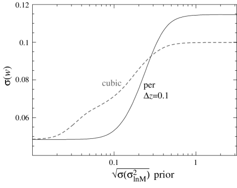
Figure 6: Prior knowledge of the scatter in the observable-mass relation at the level of $\sigma(\sigma_{\ln M}^{2})<(0.1)^{2}$ for each of the 20 redshift bins can improve dark energy constraints beyond self-calibration by a factor of 2 (solid line). This cumulative effect of independent priors is compared with the joint effect of priors on the 4 parameters of a $\sigma(B_{a})=2\sigma(\sigma_{\ln M}^{2})$ of a cubic $\sigma_{\ln M}^{2}(z)$ which captures most of the residual uncertainty in Fig. 5. The latter reflects uncertainties in $\sigma_{\ln M}^{2}$ near $z=1$.

With no self-calibration, i.e. no clustering information from the sample variance and no binning in $M^{\rm obs}$, interesting constraints on the dark energy are not possible even for the restricted evolutionary forms of Eqns. (15)-(16) if $\sigma_{\ln M}^{2}(z)$ is allowed to evolve ($N_{\sigma}\geq 2$). Even restricting the parameters to a single constant scatter ($N_{\sigma}=1$) causes a degradation to $\sigma(\Omega_{\Lambda},w)=(0.37,0.24)$.

As shown in Fig. 5 adding in the sample (co)variance information in the Fisher matrix of Eqn. (14) for a single bin in $M^{\rm obs}$ helps but still does not allow for full self-calibration of an arbitrary evolution in $\sigma_{\ln M}^{2}(z)$ even when $M^{\rm bias}$ is restricted to power law evolution. Further restricting the evolution in the mass variance to a cubic form $N_{\sigma}=4$ yields $\sigma(\Omega_{\Lambda},w)=(0.22,0.17)$ and to a constant form $N_{\sigma}=1$ yields $\sigma(\Omega_{\Lambda},w)=(0.15,0.07)$.

Employing the information contained in the shape of the counts through $M^{\rm obs}$ binning allows for a more robust self-calibration. In the case of arbitrary evolution for both the bias and the scatter $\sigma(\Omega_{\Lambda},w)=(0.03,0.21)$. With a power law form for the bias $\sigma(\Omega_{\Lambda},w)=(0.02,0.11)$; with an additional cubic form for the mass variance $\sigma(\Omega_{\Lambda},w)=(0.02,0.10)$; with a constant form for the scatter $\sigma(\Omega_{\Lambda},w)=(0.02,0.06)$.

External priors on the observable-mass distribution from simulations and cross-calibration of observables can further improve on self-calibration. Cross-calibration of cluster observables may involve a subsample of clusters which have detailed mass modeling from lensing or X-ray temperature and surface brightness profiles assuming hydrostatic equilibrium Majumdar and Mohr (2003). In Fig. 6 we explore the effect of independent priors on the 20 $\sigma_{\ln M}^{2}(z_{i})$ parameters in the power law $M^{\rm bias}$ context. Priors of the level of $\sigma(\sigma_{\ln M}^{2})=(0.1)^{2}$ would suffice to improve $\sigma(w)$ by a factor of 2. Note that the potential further improvement in $w$ errors comes from the ability to change the scatter smoothly from $z=0$ to $z\sim 1$. Since we take the priors to be independent, their cumulative effect implicitly poses a much more stringent constraint on the possible smooth evolution of $\sigma_{\ln M}^{2}$ than any one individual prior.

To better quantify the implications of the joint prior, note that the self-calibration errors on the cubic form in Fig. 5c nearly coincide with the fully arbitrary form. Taking independent priors on the 4 $B_{a}$ parameters of $\sigma(B_{a})=2\sigma(\sigma_{\ln M}^{2})$ to reflect the assumed uncertainty around $z=1$ yields the dashed curve in Fig. 6. The full improvement requires $\sigma_{\ln M}^{2}$ priors at the $(0.02)^{2}$ level and a minimum of $(0.1)^{2}$ for substantial improvements. If these priors are to come from mass modeling of observables then a fair sample of more than $\sim 100$ clusters at $z\sim 1$ with accurate masses will be required. Accurate masses will be difficult to obtain at the low threshold of $10^{14.2}h^{{-1}}M_{\odot}$ employed here.

Priors on $M^{\rm bias}$ can also improve constraints. For a completely fixed $M^{\rm bias}$, errors for an arbitrary evolution in $\sigma_{\ln M}^{2}$ are $\sigma(\Omega_{\Lambda},w)=(0.01,0.06)$. Conversely for a completely fixed $\sigma_{\ln M}^{2}$, errors for an arbitrary evolution of $M^{\rm bias}$ are $\sigma(\Omega_{\Lambda},w)=(0.02,0.13)$.

Finally to assess the possible impact of unknown trends in the mass bias and variance with mass at fixed redshift, we limit the $M^{\rm obs}$ bins to 2 separated by $\Delta\log_{10}M^{\rm obs}=0.2$ from the threshold. In this case errors for arbitrary evolution degrade slightly to $\sigma(\Omega_{\Lambda},w)=(0.03,0.26)$ and with power law mass bias and cubic variance to $\sigma(\Omega_{\Lambda},w)=(0.03,0.11)$. Thus most of the information from self-calibration comes from the small range in masses around the threshold reflecting the steepness of the mass function. The mass bias and mass variance need only be constant or slowly varying in a known way in mass across a range in masses comparable to the expected scatter for self-calibration to be effective. In any case, bins at higher masses also monitor the validity of this assumption in practice.

IV Discussion

The exponential sensitivity of number counts to the cluster mass requires a calibration of the whole observable-mass distribution before cosmological information on the dark energy can be extracted. We have shown that even in the case of an unknown arbitrary evolution in the mass bias and scatter of a Gaussian distribution there is enough information in the ratio of the counts in bins of the observable mass and their sample variance to calibrate the distribution and provide interesting constraints on the dark energy.

For the more realistic case of an unknown power law evolution in the mass bias $M^{\rm bias}$, the forecasted errors for the fiducial SPT-like survey are $\sigma(\Omega_{\Lambda},w)=(0.02,0.11)$. To further improve on these constraints, external constraints on the mass variance would need to achieve an accuracy of $\sigma(\sigma_{\ln M}^{2})<(0.1)^{2}=0.01$ on a possible evolution of the mass variance from $0\leq z\leq 1$. Note that this result is robust to the assumed true value of the scatter when quoted as a constraint on the mass variance and not the rms scatter.

However, self-calibration is not a replacement for simulated catalogues, cross-calibration techniques from so-called direct mass measurements Majumdar and Mohr (2003), and monitoring scatter in observable-observable scaling relations. It is instead an internal consistency check on their assumptions and the simplifying assumptions in this study. We have assumed that the observable-mass distribution is a Gaussian in $\ln M$ and that its parameters depend in a known way on mass at a given redshift for at least a range in masses that is greater than the expected scatter. Furthermore, for low mass clusters detected optically (e.g. Gladders and Yee (2005)) or through lensing (e.g. Wittman et al. (2003)), the assumption of a one-to-one mapping of objects identified by mass to those identified by the observable breaks down since confusion and projection will cause many small mass objects in a given redshift range to be associated with a single object in the observable (see e.g. Kim et al. (2002); Hennawi and Spergel (2005)).

Without such simplifying assumptions, true self-calibration is impossible (see e.g. Hu (2003)). Still, the ideas underlying self-calibration will be useful in revealing violations of the assumed form of the distribution of cluster observables given the cluster masses and prevent misinterpretation of the data.

Acknowledgments: We thank D. Hogg, G. Holder, A. Kravtsov, J. Mohr, A. Schulz, T. McKay, A. Vikhlinin, J. Weller, M. White for useful discussions. We also thank the organizer, A. Evrard, and the participants of the Kona Cluster meeting. This work was supported by the DOE, the Packard Foundation and CNPq; it was carried out at the KICP under NSF PHY-0114422.

References

- Ikebe et al. (2002) Y. Ikebe, T. Reiprich, H. Boehringer, Y. Tanaka, and T. Kitayama, Astron. Astrophys. 383, 773 (2002), eprint astro-ph/0112315.
- Haiman et al. (2001) Z. Haiman, J. Mohr, and G. Holder, Astrophys. J. 553, 545 (2001).
- Hu and Kravtsov (2003) W. Hu and A. Kravtsov, Astrophys. J. 584, 702 (2003), eprint astro-ph/0203169.
- Wang et al. (2004) S. Wang, J. Khoury, Z. Haiman, and M. May, Phys. Rev. D 70, 123008 (2004).
- Eddington (1913) A. Eddington, Mon. Not. R. Astron. Soc. 73, 359 (1913).
- Holder et al. (2000) G. Holder, J. Mohr, J. Carlstrom, A. Evrard, and E. Leich, Astrophys. J. 544, 629 (2000), eprint astro-ph/9912364.
- Battye and Weller (2003) R. Battye and J. Weller, Phys. Rev. D 68, 083506 (2003).
- Levine et al. (2002) E. Levine, A. Schulz, and M. White, Astrophys. J. 577, 569 (2002), eprint astro-ph/0204273.
- Hu (2003) W. Hu, Phys. Rev. D 67, 081304 (2003), eprint astro-ph/0301416.
- Majumdar and Mohr (2003) S. Majumdar and J. Mohr, Astrophys. J. 585, 603 (2003), eprint astro-ph/0208002.
- Lima and Hu (2004) M. Lima and W. Hu, Phys. Rev. D 70, 043504 (2004), eprint astro-ph/0401559.
- Jenkins et al. (2001) A. Jenkins et al., Mon. Not. R. Astron. Soc. 321, 372 (2001).
- Sheth and Tormen (1999) R. Sheth and B. Tormen, Mon. Not. R. Astron. Soc. 308, 119 (1999).
- Holder et al. (2001) G. Holder, Z. Haiman, and J. Mohr, Astrophys. J. Lett. 560, 111 (2001).
- Hu and Jain (2004) W. Hu and B. Jain, Phys. Rev. D 70, 043009 (2004), eprint astro-ph/0312395.
- Spergel et al. (2003) D. Spergel et al., Astrophys. J. Sup. 148, 175 (2003), eprint astro-ph/0302209.
- Gladders and Yee (2005) M. Gladders and H. Yee, Astrophys. J. Supp. 157, 1 (2005).
- Wittman et al. (2003) D. Wittman et al., Astrophys. J. 597, 218 (2003).
- Kim et al. (2002) R. Kim et al., Astron. J. 310, 31 (2002).
- Hennawi and Spergel (2005) J. Hennawi and D. Spergel, Astrophys. J. in press, astro (2005).