The Lyth Bound Revisited

Abstract

We investigate the Lyth relationship between the tensor-scalar ratio, $r$, and the variation of the inflaton field, $\Delta\phi$, over the course of inflation. For inflationary models that produce at least $55$ e-folds of inflation, there is a correlation between $r$ and $\Delta\phi$ as anticipated by Lyth, but the scatter around the relationship is huge. However, for inflationary models that satisfy current observational constraints on the scalar spectral index and its first derivative, the Lyth relationship is much tighter. In particular, any inflationary model with $r\lower 2.15277pt\hbox{$\;\buildrel>\over{\sim}\;$}10^{-3}$ must have $\Delta\phi\lower 2.15277pt\hbox{$\;\buildrel>\over{\sim}\;$}m_{pl}$. Large field variations are therefore required if a tensor mode signal is to be detected in any foreseeable cosmic microwave background (CMB) polarization experiment.

1 Introduction

The inflationary paradigm, promoted by Guth (1981), Linde (1982) and others, has achieved spectacular success in explaining the acoustic peak structure seen in the CMB (see Bennett et al2003 and references therein). Nevertheless, very little is known about the mechanism of inflation and how it is related to fundamental physics. The simplest mechanisms predict an adiabatic spectrum of nearly scale-invariant, Gaussian, primordial fluctuations (for reviews see Linde 1990, Lyth and Riotto 1999, Liddle and Lyth 2000). However, as Peiris et al(2003, hereafter P03) and Kinney et al(2004) demonstrate, a wide class of phenomenological inflationary models are compatible with the CMB and other cosmological data.

Given our ignorance of the underlying physics, it is worth asking what general statements can be made about inflation from particular types of observation. For example, it is well known (e.g. Lyth 1984) that the amplitude of the tensor mode CMB anisotropy fixes the energy scale of slow-roll inflation

$$V^{1/4}\approx 3.3\times 10^{16}r^{1/4}\;{\rm GeV},$$ (1)

where $r$ is the relative amplitude of the tensor and scalar modes defined as in P03. The present $95\%$ upper limit of $r<0.36$ (Seljak et al2004) gives the constraint $V^{1/4}\lower 2.15277pt\hbox{$\;\buildrel<\over{\sim}\;$}2.6\times 10^{16}\;{\rm GeV}$, or equivalently $V\lower 2.15277pt\hbox{$\;\buildrel<\over{\sim}\;$}2.2\times 10^{-11}m^{4}_{\rm pl}$.

However, a successful model of inflation must also reproduce the observed amplitude of scalar perturbations and produce a sufficiently large number of e-foldings, $N(k)$, between the end of inflation and the time that these perturbations were generated. Constraints on more general inflation models can be analysed using a set of ‘inflationary flow’ equations (Hoffman and Turner 2001, Kinney 2002, Easther and Kinney 2003, P03, Kinney et al2004) describing the evolution of a hierarchy of ‘slow-roll’ parameters. The first two slow-roll parameters are defined in terms of the Hubble parameter, $H$, during inflation by

$$\epsilon = {m^{2}_{\rm pl}\over 4\pi}\left(H^{\prime}\over H\right)^{2},$$ (2a)

$$\sigma = {m^{2}_{\rm pl}\over\pi}\left({1\over 2}{H^{\prime\prime}\over H}-\left({H^{\prime}\over H}\right)^{2}\right),$$ (2b)

where primes denote differentiation of $H(\phi)$ with respect to the inflaton $\phi$. In terms of $\epsilon$, the derivatives of $\phi$ and $H$ with respect to the number of e-foldings to the end of inflation are given by

$${d\phi\over dN}={m_{\rm pl}\over 2}\sqrt{\epsilon\over\pi},$$ (3a)

$${1\over H}{dH\over dN}=\epsilon,$$ (3b)

and $\epsilon<1$ is a necessary criterion for inflation. To second order in slow-roll parameters, the tensor-scalar ratio $r$ is given by

$$r=16\epsilon[1-C(2\epsilon+\sigma)],$$ (4)

where $C=0.08145$ (see Liddle, Parsons and Barrow 1994).

Lyth (1997) noted that for slow-roll inflation, equations (3a) and (4) can be used to relate the change in the inflaton during inflation, $\Delta\phi$, to the tensor-scalar ratio $r$, since if $\epsilon$ is roughly constant

$$\Delta\phi\sim{m_{\rm pl}\over 8}\left({r\over\pi}\right)^{1/2}\Delta N.$$ (5)

Since the Universe inflates by $\Delta N\approx 4$ during the period that wavelengths corresponding to the CMB multipoles $2\leq\ell\leq 100$ cross the Hubble radius, equation (5) leads to a bound between $\Delta\phi$ and $r$,

$$\Delta\phi>m_{\rm pl}(r/4\pi)^{1/2},$$ (6)

which we will refer to as the ‘Lyth bound.’ According to this bound, high values of $r$ require changes in $\Delta\phi$ of order $m_{\rm pl}$. In fact, equation (6) is a rather crude bound, since at least 50-60 e-foldings are required before inflation ends (see e.g. Liddle and Leach 2003). Over the full course of inflation $\Delta\phi$ could therefore exceed (6) by an order of magnitude or more.

In this paper, we investigate the Lyth bound, making as few assumptions as possible about the nature of inflation. Our aim is to establish whether a relation of the form (6) applies to general models of inflation that are compatible with observational constraints on the scalar fluctuation spectrum. Lyth (1997), Liddle and Lyth (2000), Kinney (2003) and others argue that inflation cannot be described by a low energy effective field theory if $\Delta\phi\lower 2.15277pt\hbox{$\;\buildrel>\over{\sim}\;$}m_{pl}$ and so high values of $r\sim 1$ are possible only in models for which no rigorous theoretical framework exists. Conversely, it has been argued that the Lyth bound requires $r\ll 1$ in models of inflation based on well-motivated particle physics. In Section 3, we will comment on these points and discuss the implications of the Lyth bound for inflationary model building and for future CMB experiments designed to detect tensor modes.

2 The Lyth Bound and the Inflationary Flow Equations

As mentioned in the Introduction, inflationary models can be described by an infinite hierarchy of slow roll parameters

$$\;{}^{\ell}\lambda_{H}=\left({m^{2}_{\rm pl}\over 4\pi}\right)^{\ell}{(H^{\prime})^{\ell-1}\over H^{\ell}}{d^{(\ell+1)}H\over d\phi^{(\ell+1)}}$$ (7)

that satisfy a set of ‘inflationary flow’ equations. The inflationary flow approach has been used by a large number of authors and we refer the reader to P03 and Kinney et al(2004) for a summary of the approach and for the complete set of flow equations.

The models generated here followed the prescription given in Kinney et al(2004), except that the flow hierarchy was truncated at $\ell=10$ (rather than $\ell=5$) and that successful inflationary models were required to expand by at least $N=55$ e-folds, consistent with the analysis of Liddle and Leach (2003). Inflation was deemed to end if $\epsilon>1$, in which case the models were evolved backwards by $55$ e-foldings to compute various observables, such as the tensor-scalar ratio $r$, scalar spectral index $n_{s}$, and the run in the spectral index $dn_{s}/d{\rm lnk}$ (using expressions accurate to second order in slow-roll parameters). For models in which inflation occurred at the minimum of a potential ($\epsilon\approx 0$), inflation was simply abruptly terminated and observables calculated using the slow-roll parameters at the end of inflation. Physically, such cases can be considered as examples of hybrid inflation (see Liddle and Lyth 2000) when inflation ends abruptly at some critical field value $\phi_{c}$, or as examples of brane-inflation when inflation ends at a critical inter-brane separation at which open string modes become tachyonic (see Quevedo, 2002, for a review). In practice, any models which achieved $N>200$ e-foldings were grouped into this category.

We evolved $2\times 10^{6}$ models using the above prescription. Figure 1 shows the parameters $r$, $n_{s}$ and $dn_{s}/d{\rm lnk}$ for a sample of these models plotted against each other. The distributions in these diagrams agree well with the results of previous authors and are straightforward to understand physically. More than 90% of the models are of the ‘hybrid-type’ for which $r$ is negligible (equation 4) and the scalar spectral index is $n_{s}>1$ (since the inflaton is trapped in the minimum of a potential). Of the remaining models, those colour coded in blue in Figure 1 have $r<0.36$ and so are consistent with current constraints on the tensor-scalar ratio. The middle panel of Figure 1 shows that these models span a wide range of $n_{s}$ and $dn_{s}/d{\rm lnk}$.

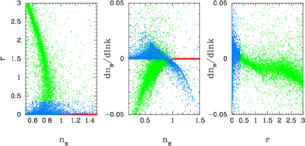
Figure 1: The tensor-scalar ratio, $r$, scalar spectral index, $n_{s}$, and run in the spectral index, $dn_{s}/d{\rm ln}k$, plotted against each other for realizations of the inflationary flow equations described in the text. The colour coding is as follows: the majority of models (colour coded red) inflate forever with $\epsilon=0$ and have negligible tensor component. In the remaining models, inflation ends when $\epsilon=1$ after at least 55 e-folds of inflation. These models have been colour coded blue if $r\leq 0.36$ (the observational upper limit derived by Seljak et al2004) and green if $r>0.36$.

Figure 2 shows plots of $|\Delta\phi|$ over the final $55$ e-foldings of inflation computed from equation (3a) plotted against the tensor-scalar ratio $r$. The figure to the left shows $\Delta\phi$ for all models within the designated ranges of the abscissa and ordinate, colour coded so that hybrid-type models are plotted in red, with the rest of the models plotted in blue. This Figure shows that for general inflationary models, there is no well defined Lyth relation of the form (6). Models can be found, for example, with $r\lower 2.15277pt\hbox{$\;\buildrel>\over{\sim}\;$}1$ and $\Delta\phi/m_{\rm pl}$ in the range $0.1$–$0.2$. Likewise, models can be found with low values of $r\lower 2.15277pt\hbox{$\;\buildrel<\over{\sim}\;$}10^{-4}$ and $\Delta\phi/m_{\rm pl}$ well in excess of unity. However, on closer inspection, one finds that models lying in these regions of the diagram have unusual scalar spectral indices. In the former case, the models have blue spectra with $n_{s}>1.1$, and in the latter case the models have red spectra with $n_{s}<0.8$. It is therefore interesting to plot $r$ against $\Delta\phi$ only for those models that satisfy observation constraints on the shape of the scalar power spectrum.

The tightest observational constraints on $n_{s}$ and $dn_{s}/d{\rm lnk}$ at present come from combining observations of the CMB anisotropies, with observations of the matter power spectrum deduced from galaxy redshift surveys and from Ly$\alpha$ lines in the spectra of high redshift quasars (see e.g. Viel et al2004, Seljak et al2004). The recent results of Seljak et algive approximate $2\sigma$ ranges of

$$\left.\begin{array}[]{l}\quad 0.92<n_{s}<1.06\\ -0.04<dn_{s}/d{\rm lnk}<0.03\end{array}\right\}$$

(see Figure 3 of Seljak et al2004). Figure 2b shows $r$ and $\Delta\phi$ for the subset of models that satisfy the constraints given in (8). (In fact, although we have imposed a constraint on $dn_{s}/d{\rm lnk}$, it is the constraint on $n_{s}$ that has the most significant effect in defining the distribution of points in Figure 2b.) The models plotted in Figure 2b now delineate a much tighter relationship between $r$ and $\Delta\phi$, which can be approximated for $r\lower 2.15277pt\hbox{$\;\buildrel>\over{\sim}\;$}10^{-3}$ by

$${\Delta\phi\over m_{\rm pl}}\approx 6r^{1/4}.$$ (8)

This relation is our reformulation of the Lyth bound (6).

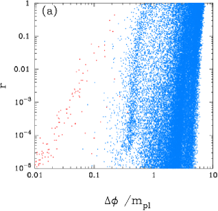
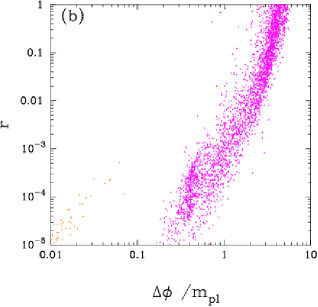
Figure 2: The absolute value of $\Delta\phi$ over the last $55$ e-folds of inflation plotted against the tensor-scalar ratio, $r$. Figure 2a shows all models colour coded so that hybrid-type models are shown in red and the rest are shown in blue. Figure 2b shows the subset of models that satisfy the observational constraints on $n_{s}$ and $dn_{s}/d{\rm ln}k$ discussed in the text. The colour coding in this figure is as follows: hybrid-type models are shown in orange and the rest of the models are shown in magenta.

3 Implications

Present observations set the constraint $r<0.36$ (Seljak et al2004). To improve on this limit significantly will require more sensitive CMB polarization experiments than those done so far. The Planck satellite should be able to achieve a limit of $r\lower 2.15277pt\hbox{$\;\buildrel<\over{\sim}\;$}0.1$ by measuring the B-mode polarization spectrum, but despite the fact that Planck will survey the entire sky from space it is limited in sensitivity by the small number of polarization sensitive detectors. Ground based B-mode optimised experiments, using either bolometer arrays (CLOVER, Taylor et al2004), or large arrays of coherent detectors (QUIET ) are currently being designed that should be able to set limits of $r\sim 10^{-2}$ in the presence of realistic foregrounds. For $r\lower 2.15277pt\hbox{$\;\buildrel<\over{\sim}\;$}10^{-2}$, B-mode anisotropies caused by gravitational lensing of the CMB (Zaldarriaga and Seljak 1998) will need to be subtracted in order to extract an inflationary tensor component. However, there are limits on how accurately a lensing contribution can be subtracted. For example, even in the absence of instrumental noise and foregrounds, Lewis et al(2002) find that a survey of the sky of radius $15^{\circ}$ leads to a limit of $r\sim 3\times 10^{-4}$ from the sample variance of the lens-induced B-modes. This limit could potentially be improved by a factor of $10$ with a noiseless all sky survey (Kesden et al2002, Knox and Song 2002), and perhaps by another factor of $10$ if the lens-induced B-modes can be mapped accurately enough to reconstruct the deflection field (Hirata and Seljak 2003). Comparing with equation (1), under optimistic assumptions the lowest energy scale of inflation that can be probed by CMB B-mode polarization measurements is $V^{1/4}\lower 2.15277pt\hbox{$\;\buildrel>\over{\sim}\;$}1\times 10^{15}\;{\rm GeV}$. More realistically, the next generation of CMB experiments such as CLOVER and QUIET may reach $r\sim 10^{-2}$, corresponding to an energy scale of $V^{1/4}\sim 1\times 10^{16}\;{\rm GeV}$.

Figure 2b shows that to produce a detectable tensor component in any foreseeable CMB experiment, inflation must necessarily involve large field variations, $\Delta\phi/m_{\rm pl}\lower 2.15277pt\hbox{$\;\buildrel>\over{\sim}\;$}1$. In fact, the dependence of $\Delta\phi$ on $r$ in Figure 2b is so steep that we would need to achieve $r\lower 2.15277pt\hbox{$\;\buildrel<\over{\sim}\;$}10^{-4}$ to probe inflationary models with low field variations of $\Delta\phi/m_{\rm pl}\lower 2.15277pt\hbox{$\;\buildrel<\over{\sim}\;$}0.1$. Thus, for the foreseeable future, we will only be able to test high-field models of inflation. Furthermore, it may well prove impossible, given realistic polarized foregrounds, to probe small-field models of inflation using the CMB.

It is often argued (e.g. Lyth 1997) that the effective potential can be written as a power series

$$V(\phi)=V_{0}+\alpha\phi+{m^{2}\over 2}\phi^{2}+{\beta\over 3}\phi^{3}+{\lambda\over 4}\phi^{4}+\sum_{n}\lambda_{n}{\phi^{4+n}\over m_{\rm pl}^{n}},$$ (9)

with $\lambda_{n}\sim{\cal O}(1)$, and hence that an effective field theory description of inflation becomes invalid for field values $\phi\lower 2.15277pt\hbox{$\;\buildrel>\over{\sim}\;$}m_{\rm pl}$. However, as Linde (2004) points out, quantum gravity corrections to $V(\phi)$ should become large only for $V(\phi)>m_{\rm pl}^{4}$ , not $\phi>m_{\rm pl}$ as inferred from equation (9). This is the rationale behind chaotic inflation models such as the simple $\lambda\phi^{4}$ model (which is now excluded observationally at about the $3\sigma$ level). However, it has proved difficult to find realisations of chaotic inflation motivated by realistic particle physics. For example, realising the conditions for slow-roll inflation for either large or small field variations has been a long standing problem in $N=1$ supergravity. This may, however, simply reflect our lack of understanding of supergravity. For example, it has been pointed out recently that chaotic inflation can be realised in supergravity models if the potential has a shift symmetry (Kawasaki et al2000, Yamaguchi and Yokoyama 2001), i.e. the inflaton potential does not depend on the imaginary part of a complex field $\Phi$ (see Linde 2004 for a more detailed discussion). It may therefore be possible to construct particle physics motivated models of inflation with $\Delta\phi\lower 2.15277pt\hbox{$\;\buildrel>\over{\sim}\;$}1$. Understanding the physics behind such high-field models is important, for as we have shown in this paper they are the only class of inflationary models that can be probed by CMB B-mode polarization experiments in the foreseeable future.

Acknowledgments: The research of GPE is supported by the UK Particle and Astrophysics Research Council. KM would like to thank the Institute of Astronomy for their hospitality during a summer visit when part of this work was done.

References

References

- [1]
- [2] [] Bennett C.L., et al, 2003, Ap J. Suppl. Ser., 148, 1.
- [3]
- [4] [] Easther R., Kinney W.H., 2003, Phys. Rev.D, 67, 043511.
- [5]
- [6] [] Guth A.H., 1981, Phys. Rev.D, 23, 347.
- [7]
- [8] [] Hirata C.M., Seljak U., 2003, Phys. Rev.D, 68, 083002.
- [9]
- [10] [] Hoffman M.B., Turner M.S., 2001, Phys. Rev.D, 64, 023506.
- [11]
- [12] [] Kawasaki M., Yamaguchi M., Yanagida T., 2000, Phys. Rev.L, 85, 3572.
- [13]
- [14] [] Kesden M., Cooray A., Kamionkowski M., 2002, Phys. Rev.L, 89, 0113041.
- [15]
- [16] [] Kinney W.H., 2002, Phys. Rev.D, 66, 083508.
- [17]
- [18] [] Kinney W.H., 2003, New Astronomy Reviews, 1387.
- [19]
- [20] [] Kinney W.H., Kolb E.W., Melchiorri A., Riotto A., 2004, Phys. Rev.D, 69, 1035161.
- [21]
- [22] [] Knox, L., Song, Y-S., 2002, Phys. Rev.L, 89, 0113031.
- [23]
- [24] [] Lewis A., Challinor, A., Turok N., 2002, Phys. Rev.D, 65, 023505.
- [25]
- [26] [] Liddle A.R., 2003 Phys. Rev.D, 68, 103504.
- [27]
- [28] [] Liddle A.R., Lyth D.H., 2000, ‘Cosmological Inflation and Large-Scale Structure, Cambridge University Press, Cambridge.
- [29]
- [30] [] Liddle A.R., Leach S.M., 2003, Phys. Rev.D, 68, 103503.
- [31]
- [32] [] Liddle A.R., Parsons P., Barrow J.D., 1994, Phys. Rev.D, 50, 7222.
- [33]
- [34] [] Linde A.D., 1982, Phys. Lett. B, 108, 389.
- [35]
- [36] [] Linde A.D., 1990, Particle Physics and Inflationary Cosmology, Hardwood Academic Publishers.
- [37]
- [38] [] Linde A.D., 2004, hep-th/0402051.
- [39]
- [40] [] Lyth D.H., 1984 Phys Lett B, 147, 403L.
- [41]
- [42] [] Lyth D.H., 1997 Phys. Rev. Lett., 78, 1861.
- [43]
- [44] [] Lyth D.H., Riotto A.A., 1999, Physics Reports, 314, 1.
- [45]
- [46] [] Peiris H.V., et al2003, Ap. J. Suppl., 148, 213.
- [47]
- [48] [] Quevedo F., 2002, Class. Quantum Gravity, 19, 5721.
- [49]
- [50] [] Seljak U., et al, 2004, submitted to Phys. Rev.D (astro-ph/0407372).
- [51]
- [52] [] Taylor, A.C. et al, 2004, (astro-ph/0407148).
- [53]
- [54] [] Viel M., Weller J., Haehnelt M.G., 2004, MNRAS, 355, L23.
- [55]
- [56] [] Wang L., Mukhanov V.F., Steinhardt P.J., 1997, Phys Lett B, 414, 18.
- [57]
- [58] [] Yamaguchi M, Yokoyama J., 2001, Phys. Rev.D, 63, 043506.
- [59]
- [60] [] Zaldarriaga, M., Seljak, U., 1998, Phys. Rev.D, 58, 023003.
- [61]