Forward modeling of stellar coronae:
from a 3D MHD model to synthetic EUV spectra

Abstract

A forward model is described in which we synthesize spectra from an ab-initio 3D MHD simulation of an outer stellar atmosphere, where the coronal heating is based on braiding of magnetic flux due to photospheric footpoint motions. We discuss the validity of assumptions such as ionization equilibrium and investigate the applicability of diagnostics like the differential emission measure inversion. We find that the general appearance of the synthesized corona is similar to the solar corona and that, on a statistical basis, integral quantities such as average Doppler shifts or differential emission measures are reproduced remarkably well. The persistent redshifts in the transition region, which have puzzled theorists since their discovery, are explained by this model as caused by the flows induced by the heating through braiding of magnetic flux. While the model corona is only slowly evolving in intensity, as is observed, the amount of structure and variability in Doppler shift is very large. This emphasizes the need for fast coronal spectroscopy, as the dynamical response of the corona to the heating process manifests itself in a comparably slow evolving coronal intensity but rapid changes in Doppler shift.

1. Introduction

Since the discovery that the outer atmosphere of the Sun, the corona, is much hotter than the photosphere (Grotrian, 1939; Edlén, 1942) it remains a mystery what heats the coronae of the Sun and other cool stars to more than a million K. During the last decade a wealth of coronal data was collected through remote sensing, especially with the help of the Yohkoh, SOHO and TRACE space missions. Since the beginning of coronal physics there have been countless suggestions of coronal heating processes, as to be found in the proceedings of conferences on coronal heating, e.g. Ulmschneider et al. (1991) or the SOHO 15 meeting (Walsh et al., 2004). There was never a lack of suggestions — the problem is how to prove or disprove a model with the help of observations.

Observations of the corona provide us with the flux and energy of photons. To test a model one might use an inversion of the observations to derive e.g. temperatures and densities, and compare this to the modeled plasma parameters. In such an inversion procedure one has to make implicit assumptions and often the inversion problem is ill-posed (e.g. Judge & McIntosh, 1999; McIntosh, 2000). The other major approach is forward modeling. Based on a model one derives not only the plasma parameters, but also the photon spectra resulting from the model atmosphere. Like an inversion, also a forward model is based on assumptions, but usually the assumptions are more easy to control in a forward model approach. In the past numerous forward models have been applied to study various coronal phenomena, like transition region redshifts (e.g. Hansteen, 1993), the connectivity of the atmosphere (e.g. Wikstøl et al., 1998), or catastrophic cooling in loops (e.g. Müller et al., 2004). Likewise the inversion approach can allow a detailed comparison, when treated with care. For example Priest et al. (1998) compared the temperature profiles from various loop heating models and compared these to the temperature profile derived for a large isolated loop as inverted from Yohkoh soft X-ray observations.

There are many observational challenges a coronal model has to explain, and we will here only name a few which are of relevance for our work. The structures are much more smooth in the corona than in the transition region (e.g. Reeves, 1976). The emission measure, i.e. the intrinsic capability for a volume at a given temperature to radiate, is strongly increasing from the transition region down to the chromosphere (e.g. Dowdy et al., 1986). The middle transition region shows persistent redshifts (Doschek et al., 1976), while the low corona shows a net blueshift (Peter, 1999). The unresolved motions are largest in the middle transition region (e.g. Chae et al., 1998a). The temporal variability of the line intensities is largest in the middle transition region (e.g. Brković et al., 2003). Here we cannot give a full list of references relevant for coronal heating based on data from Yohkoh, SOHO and TRACE, but we would like to emphasize the usefulness of spectroscopic investigations using the SUMER EUV spectrometer on SOHO (Wilhelm et al., 1995, 1997)

In the light of the new observations provided in the recent years it is especially encouraging that complex three-dimensional ab-initio models for the corona based on magnetohydrodynamics (MHD) are becoming available (Gudiksen & Nordlund, 2002, 2005a, 2005b). In this work we calculate the EUV spectra from these models, which allows us to perform a detailed comparison to observations. The aim of this paper is to describe the validity and applicability of the approach chosen here to synthesize the EUV spectra and to show the huge potential of this forward modeling approach. First results on the spectral synthesis have already been published in Peter et al. (2004).

We will first give a very quick introduction to the coronal MHD model (Sect. 2), before we describe the synthesis of the EUV spectra in Sect. 3. The validity and applicability of our approach will be discussed in Sect. 4 and finally in Sect. 5 we will investigate the relation of our approach to real solar observations, like the morphology, average line shifts and widths or the differential emission measure.

2. 3D MHD model of coronal structures

Here we will only give a very brief overview on the basics of the 3D MHD model underlying our spectral synthesis. A detailed description of the model can be found in Gudiksen & Nordlund (2005a, b).

In this model the heating of the corona is due to braiding of magnetic flux as a consequence of photospheric motions, as suggested first by Parker (1972). The braided magnetic field gives rise to currents which are then dissipated through Ohmic heating. The horizontal motions in the photosphere are constructed based on a Voronoi-tessellation (e.g. Okabe et al., 1992). This flow field reproduces the geometrical pattern and the amplitude power spectrum of the velocity and the vorticity.

The computational box contains a volume of $60\times 60$ Mm² in the horizontal directions and 37 Mm vertically covering the whole atmosphere from the photosphere to the corona with a non-equidistant grid of 150³ points. A 5’th order in space, 3rd order in time, fully compressible 3D magneto-hydro-dynamics (MHD) code on a staggered non-equidistant mesh is used, including classical heat conduction along the magnetic field (Spitzer, 1956) and a cooling function of optically thin radiative losses. A Newtonian cooling scheme is used to keep the atmosphere near a prescribed temperature profile in the photosphere and chromosphere.

The simulation starts with an initial condition with a magnetic field from a potential field extrapolation based on an observed magnetogram, scaled down to fit into the computational box. The heating through braiding of magnetic flux rapidly leads to a corona which is intermittent in space and time, typically reaching temperatures of about $10^{6}$ K. On average the heating is concentrated very much at the bottom of the computational domain in the chromosphere and drops exponentially towards larger heights. The heat flux into the corona of about 2000–8000 W/m² is comparable to the energy losses derived from observations (e.g. Withbroe & Noyes, 1977). The amount of heating in this model is only a lower limit, as the heating would stay constant or increase with increased spatial resolution (Hendrix et al., 1996; Galsgaard & Nordlund, 1996), and the initial conditions and the driver are constructed in a way as to induce a minimum of stress in the magnetic field (see discussion in Gudiksen & Nordlund, 2005a).

For the spectroscopic investigations in this paper we use only the last ${\sim}20$ minutes of the whole simulated time span of ${\sim}50$ minutes, to ensure that our results are sufficiently independent of the initial conditions. Thus in this paper the time $t{=}0$ minutes refers to a time ${\sim}30$ minutes into the MHD simulation.

3. Calculation and analysis of synthetic spectra

To study the spectral line properties from the MHD calculation we first calculated the emissivities of a number of emission lines from the transition region and low corona at each grid point. Using these emissivities and the velocities from the MHD calculation we calculate the spectrum for each line at each grid point. Finally we integrate the spectra along a line-of-sight in order to obtain spatial maps of line intensity, shift and width. Similarly we also compute the average spectra from the box to study the average emission line properties. Thus the spectra synthesized from the MHD calculation are directly comparable to observations of EUV spectra, on a statistical basis, of course.

The lines used in this paper are listed in Table 1. All these lines are optically thin, at least at disk center — only this allows the concept of synthesizing the spectra as outlined above without accounting for radiative transport (see also Sect. 4). The lines have been chosen using two criteria. Firstly we wanted to span the whole range of temperatures in the transition region from the chromosphere to the corona, i.e. from 10⁴ to 10⁶ K. And secondly the lines should be observable with SUMER to allow for a comparison with the observed properties of the line profile.

3.1. Line emissivity

The line emissivities at each grid point are calculated under the assumption of ionization equilibrium (cf. Sect. 4.2). To calculate the various populations of excitation and ionization states we use the atomic data package CHIANTI (Version 4.02; see Dere et al., 1997; Young et al., 2003). Because of computational time we first create a look-up table for a large number of temperatures and densities, and then read from this table to extract the line emissivities.

The lines considered in this paper (Table 1) are predominantly excited by electron collisions and de-excited by spontaneous emission. The emissivity (integrated over the line profile, i.e. energy per time and volume) is then given by

$$\varepsilon=h\nu\,n_{2}A_{21}~{},$$ (1)

where $h\nu$ is the energy of the transition, $n_{2}$ is the population number density of the upper level and $A_{21}$ is the Einstein coefficient for spontaneous emission to the lower level. Eq. (1) can be rewritten as

$$\varepsilon=G(T,n_{e})~{}n_{e}^{2}~{},$$ (2)

with the electron number density $n_{e}$ and a function $G(T,n_{e})$ defined as

$$G(T,n_{e})=h\nu\ A_{21}\cdot\frac{n_{2}}{n_{e}~{}n_{\rm{ion}}}\cdot\frac{n_{\rm{ion}}}{n_{\rm{el}}}\cdot\frac{n_{\rm{el}}}{n_{\rm{H}}}\cdot\frac{n_{\rm{H}}}{n_{e}}~{}.$$ (3)

The terms describe the excitation of the line, the ionization of the respective ion, the elemental abundance and the degree of ionization of the plasma. The number density of ions in the respective ionization state is $n_{\rm{ion}}$, the number density of the respective element is $n_{\rm{el}}$ and $n_{\rm{H}}$ denotes the number density of hydrogen.

The first term of (3), $h\nu{}A_{21}$, is a constant given by atomic physics.

Because the excitation of the lines considered here is due to electron collisions, the population of the upper level $n_{2}/n_{\rm{ion}}$ is basically proportional to the electron density. This is true only for density insensitive lines and for a certain range of densities. Thus the second term of (3) depends mainly on temperature, but generally also on density. We fully account for the temperature and density dependence when calculating this term using CHIANTI.

Under the assumption of ionization equilibrium the ionization degree $n_{\rm{ion}}/n_{\rm{el}}$ in (3) depends only on temperature and we use the values calculated by Mazzotta et al. (1998) as tabulated in the CHIANTI package. Of course, this is a strong assumption in a dynamic atmosphere like investigated in the present MHD model. Nevertheless in large parts of the atmosphere under investigation here this assumption can be considered a good first step. This will be discussed separately in Sect. 4.2.

In evaluating Eq. (3) we use constant abundances $n_{\rm{el}}/n_{\rm{H}}$ throughout the computational box and adopt the most recent solar photospheric values as tabulated in the CHIANTI package. Especially we do not account for the change of abundances (by a factor of 2 to 3) that is to be expected in the chromosphere, i.e. the FIP effect (e.g. von Steiger et al., 2000).

In a fully ionized plasma with hydrogen and 10% Helium the value of $n_{\rm{H}}/n_{e}$ is about 0.8. Here we use CHIANTI to calculate this term depending on the degree of ionization, i.e. on temperature.

From this discussion we see that the contribution function $G(T,n_{e})$ as defined in (3) depends only weakly on density when selecting an appropriate line. Thus it is often referred to as $G(T)$. Mainly because of the ionization equilibrium the function $G(T,n_{e})$ strongly peaks in temperature. Based on the ionization equilibrium calculations a canonical value for the width of the contribution function is 0.3 in $\log{}T$ (cf. Sect. 4.1). For density insensitive lines, i.e. $G{=}G(T)$, the emissivity (2) reflects that the optically thin radiative losses are proportional to the density squared.

To evaluate the emissivity (2) at each grid point of the MHD calculation we finally compute the electron density $n_{e}$ from the mass density $\rho$ of the MHD calculation using the degree of ionization, again as obtained from CHIANTI. By an integration along the line-of-sight we can then calculate the energy flux density in a given emission line out of our computational box, e.g. in units of W/m² These can be easily converted into line radiances as observed e.g. at the location of SOHO.

Table 1Emission lines synthesized in this study.

		formation temperature: log $T$ [K]				FWHM
		ion.eq.	excitation	DEM	MHD	$\Delta\log T$
Si II	1533	4.60	4.36	4.08	4.25	–
Si IV	1394	4.81	4.85	4.82	4.90	0.29
C II	1335	4.67	4.57	4.23	4.64	0.22
C III	977	4.78	–	4.71	4.84	0.29
C IV	1548	5.00	5.00	5.02	5.11	0.25
O IV	1401	5.27	5.14	5.15	5.18	0.32
O V	630	5.38	5.35	5.40	5.44	0.28
O VI	1032	5.45	5.44	5.50	5.60	0.23
Ne VIII	770	5.81	5.76	5.82	5.89	0.16
Mg X	625	6.04	6.01	6.01	6.06	0.17

The line formation temperatures given here are as following from different methods: maximum of ionization fraction (“ion.eq.”), maximum of ionization fraction accounting for collisional excitation (“excitation”), constant pressure DEM inversion using CHIANTI (“DEM”) and based on emissivities of the present MHD model (“MHD”). The rightmost column gives the width of the respective contribution function in temperature as following from the present work in a logarithmic scale. See Sect. 4.1 for a detailed discussion.

3.2. Synthetic spectral profiles

For convenience we calculate all spectral profiles with the wavelength given in units of (Doppler) velocities.

To calculate the emission line profiles at each grid point we assume that the line profile has a thermal width $w_{\rm{th}}$ according to the temperature $T$ as obtained from the MHD calculation at the respective grid point,

$$w_{\rm{th}}=\left(\frac{2\,k_{\rm{B}}~{}T}{m_{i}}\right)^{1/2}~{}.$$ (4)

Here $k_{\rm{B}}$ is Boltzmann’s constant and $m_{i}$ is the atomic mass of the respective ion.

Furthermore the line is Doppler shifted by the line-of-sight velocity at the respective grid point. In this paper we concentrate on a vertical line-of-sight, as we would like to compare our results of average synthesized Doppler shifts to observations of solar disk center Doppler shifts. Thus we use the vertical component of the velocity $v_{\rm{v}}$ from the MHD calculation.

Now the line profile $I_{v}$ at each grid point is given by

$$I_{v}=I_{\rm{peak}}\exp\left(-\,\frac{(v-v_{\rm{v}})^{2}}{w_{\rm{th}}^{2}}\right)~{}.$$ (5)

For such a Gaussian with an exponential width $w_{\rm{th}}$ the peak intensity $I_{\rm{peak}}$ is related to the total intensity $I_{\rm{tot}}$, i.e. integrated over wavelength (or here velocity), by

$$I_{\rm{tot}}=\sqrt{\pi}\,I_{\rm{peak}}\,w_{\rm{th}}~{}.$$ (6)

The total intensity $I_{\rm{tot}}$ is given through the emissivity (2) as discussed in Sect. 3.1.

Thus we can use (5) to calculate the spectrum at each grid point as viewed along the (vertical) line-of-sight. To obtain the total spectrum we integrate along the line-of-sight,

$$I_{v}^{\rm{synth}}=\int_{\rm{line-of-sight}}I_{v}~{}{\rm{d}}l~{}.$$ (7)

This yields two dimensional maps of spectra as they would be obtained if an EUV spectrometer like SUMER would perform a raster scan. Thus we name these spectra $I_{v}^{\rm{synth}}$, synthetic spectra. These are (in general) not Gaussian, even though in the present study they are mostly close to Gaussian.

The analysis of the synthetic spectra is similar to the procedure for observed spectra: we calculate line intensity, position and width of $I_{v}^{\rm{synth}}$ at each location of the spatial maps. For observed solar spectra it is preferable (and almost always necessary) to perform a Gaussian fit to derive these parameters, which is mainly because of the noise in the data. As our synthetic spectra are noise-free and very close to Gaussians it is sufficient to calculate the profile moments with respect to wavelength (or here velocity $v$). Then line intensity, shift and width are given by

$$I^{\rm{synth}} = \int I_{v}^{\rm{synth}}~{}{\rm{d}}v~{},$$ (8)

$$v^{\rm{synth}} = \frac{1}{I^{\rm{synth}}}\int v~{}I_{v}^{\rm{synth}}~{}{\rm{d}}v~{},$$ (9)

$$w^{\rm{synth}} = \frac{1}{I^{\rm{synth}}}\left(2\int(v-v^{\rm{synth}})^{2}~{}I_{v}^{\rm{synth}}~{}{\rm{d}}v\right)^{1/2}~{}.$$ (10)

It is easy to check that this indeed returns the desired parameters if $I_{v}^{\rm{synth}}$ whould be exactly Gaussian. Examples of maps of synthesized Doppler shifts and intensities are shown in 5 (panels a/$\alpha$ and b/$\beta$, respectively; panels c/$\gamma$ and d/$\delta$ show the box as seen from the sides in intensity; Latin and Greek letters label maps about 7 minutes apart in time).

When analyzing the line width in observations one usually subtracts the thermal line with as defined in (4) assuming the line is formed at a single temperature $T_{\rm{line}}$. Here we use the temperatures as derived from the analysis of line formation temperatures (see Sect. 4.1; column “MHD” in Table 1). This results in the non-thermal line width or non-thermal velocity $w^{\rm{synth}}_{\rm{nt}}$ characterizing the unresolved motions. This includes the velocity fluctuation along the line-of-sight.

$$w^{\rm{synth}}_{\rm{nt}}=\left(\left(w^{\rm{synth}}\right)^{2}~{}-~{}\frac{2\,k_{\rm{B}}~{}T_{\rm{line}}}{m_{i}}\right)^{1/2}~{}.$$ (11)

It is important to note that when synthesizing the spectrum at a given grid point we use the temperature at that grid point to evaluate the thermal width following (4). After integration along the line-of-sight we subtract the thermal width in (11) as to be expected at an average $T_{\rm{line}}$ in the line formation region. Thus our analysis of the data follows closely the analysis of “real” observational data.

3.3. Differential emission measure analysis

The concept of the (differential) emission measure (DEM or EM) is widely used in the analysis of stellar and solar optically thin plasmas. Thus we will apply this tool also to our synthetic spectra.

Following the discussion in Sect. 3.1 the line flux (i.e. the energy flux of the photons, e.g. in W/m²) at a given location on the Sun is given by a height integration of the emissivity (2).

$$F~{}=~{}\int G(T,n_{e})~{}n_{e}^{2}~{}{\rm{d}}h~{}.$$ (12)

To perform the DEM analysis one has to make the assumption that the integration over height can be substituted by an integration over temperature, i.e.

$$F~{}=~{}\int G(T,n_{e})~{}{{\rm{DEM}}}~{}{\rm{d}}T~{}.$$ (13)

with the differential emission measure

$${{\rm{DEM}}}~{}=~{}n_{e}^{2}~{}\frac{{\rm{d}}h}{{\rm{d}}T}~{}.$$ (14)

It is important to note that this implicitly assumes that the temperature varies monotonically with height. The highly structured nature of the corona, of course, proves this assumption untenable (see Sect. 4.3 and Sect. 5.5).

Using a suitable set of lines covering a large range of temperatures one can derive the DEM from the observed or synthesized line intensities. To account for the density dependence of $G$ one has to make an assumption on the density in the atmosphere. We use the approximation of constant pressure, which is most common for the transition region because of its small thickness compared to the pressure scale height. To perform the DEM inversion we employed the CHIANTI package. This also returns the respective line formation temperatures (see Sect. 4.1).

We would like to stress here that the inversion of ${{\rm{DEM}}}(T)$ is an ill-posed problem (e.g. Judge & McIntosh, 1999; McIntosh, 2000) and that one has to be very careful in the selection of lines, e.g. with respect to the iso-electric sequence (Del Zanna et al., 2002). However, our emphasis in this paper is not on a best possible ${{\rm{DEM}}}$ inversion — we are applying the ${{\rm{DEM}}}$ inversion to our data only to show that our synthetic spectra yield a ${{\rm{DEM}}}$ distribution with temperature similar to observed ones when applying standard techniques.

4. Validation of the approach

The spectral synthesis as outlined above presents us with two major limitations. The formation of lines at low temperatures is not well representsed and the ionization equilibrium is a strong assumption.

The MHD model is not including a self-consistent treatment of the chromosphere including radiative transport, but is using a Newton cooling mechanism to keep the lower part of the computational box at a prescribed chromospheric temperature profile. Thus any diagnostics of the plasma at temperatures below, say, $10^{4}$ K is meaningless, and will not be touched upon in this paper.

For the lines formed in the low transition region, below $\log{T}{\approx}4.5$, we will be confronted with another problem. Because of the very steep rise of density from the transition region down into the chromosphere, through (2) the formation of these lines is shifted towards considerably lower temperatures, as will be discussed in Sect. 4.1. Whether this is an artefact of the MHD model used here, or a general property of outer stellar atmospheres can only be clarified when more complex coronal models become available. If indeed these low temperature lines are formed well below the temperature of peak ion fraction (cf. 1a), this would have serious impact on the interpretation of observations of these lines.

For the present study it seems that ionization equilibrium is a good assumption as outlined in Sect. 4.2. Despite velocities of some 10 or 20 km/s in the middle transition region this assumption holds. Previous studies found contrary results, but they neglected the back-reaction of the flow on the temperature gradient. Future studies with more violent flows, however, will have to consider departures from ionization equilibrium, as is known e.g. from the modeling of explosive events or reconnection (e.g. Roussev et al., 2001; Roussev & Galsgaard, 2002). Those models, however, where only 2D-MHD models and the non-equilibrium ionization was solved properly only in 1D along a line-of-sight aligned with the outflow from a reconnection site. 1D codes with non-equilibrium ionization exist since quite a while (e.g. Hansteen, 1993), but to move on to a full 3D treatment is a major step.

4.1. Line formation temperatures

The function $G$ as used in (2) is a function sharply peaked in temperature. Thus one can define a line formation temperature. As $G(T)$ is mainly determined by the fractional density of the ionization stage, one often uses the peak temperature of the ionization fraction $n_{\rm{ion}}/n_{\rm{el}}$. In Table 1 values as following from the ionization equilibrium calculation of Landini & Monsignori Fossi (1990) are listed (column “ion.eq.”). One can go one step further and also include the temperature dependence of the collisional excitation process by using the peak of the upper level population in a simple density independent way $n_{\rm{ion}}/n_{\rm{el}}\,{\cdot}\,T^{-1/2}\exp(-h\nu/k\,T)$ — values obtained by Chae et al. (1998a) and Chae et al. (1998b) are listed in the column “excitation” of Table 1. However, $G$ depends also on density, which is not accounted for by these two approaches. A DEM inversion as discussed in Sect. 3.3 returns the line formation temperatures for a constant pressure atmosphere, implicitly assuming a simple 1D stratified atmosphere (column “DEM” in Table 1).

For the analysis of the synthetic spectra from our MHD model we do not have to make all these simplifying assumptions, but we can calculate directly the contribution function of the respective lines. Employing the procedure outlined in Sect. 3.1 the emissivity is calculated at each grid point. Based hereupon we integrate the total emission from the computational box in each line in small temperature intervals (actually, we use intervals in $\log_{10}$ of temperature). As the atmosphere in our model is highly structured, the volume each temperature interval covers is not necessarily spatially connected. From this we can compute the contribution of the respective line as a function of temperature.

Figure 1.— Contribution to the emissivity as a function of temperature for a number of lines (crosses). Except for Si II the contribution in $\log T$ is roughly represented by a Gaussian. Gaussian fits are over-plotted as solid lines and the respective full widths at half maximum (FWHM) of the Gaussians are given as bars. The FWHM values are also given on a $\log_{10}$ scale with the bars. The vertical lines represent the first moment of the contribution function, used as a line formation temperature in this paper. See Sect. 4.1.

These contribution functions are plotted as crosses in 1 for a number of lines. We have used intervals of 0.02 in $\log_{10}T$, but the results change only slightly for other values. Except for Si II the contribution in $\log{T}$ is roughly represented by a Gaussian. To account also for the asymmetries in the contribution function, which are due to the highly structured nature of the atmosphere, we use the first moment of the contribution function in $\log{T}$ to describe the line formation temperature (this is practically identical to the center of the respective Gaussian fit, cf. 1).

A canonical value for the range of temperatures contributing to transition region lines is about 0.3 in $\log{T}$, i.e. 0.3 dex. The full width at half maximum (FWHM) of the Gaussian fits is usually a bit smaller than that, but 0.3 dex seems to be a good choice, even for a highly structured atmosphere as considered here (cf. 1 and rightmost column of Table 1).

The contribution function for the “coolest ion” discussed in this paper, Si II, is far from being Gaussian or even having a well pronounced peak in temperature (1a). There is a small secondary peak just below $\log{T}{=}4.6$, where the ion fraction peaks (cf. Table 1), but below $\log{T}{=}4.4$ the contribution of Si II rises and well exceeds the value at the temperature of peak ion fraction. This is due to the density dependence of the contribution function $G$ (also the DEM inversion using CHIANTI gives a low temperature of $\log{T}{=}4.08$ for this ion, cf. Table 1). The bulk part of the Si II emission originates from temperatures below $\log{T}{=}4.4$, where the ion fraction of Si⁺ is still low. As there is no self-consistent treatment of the upper chromosphere, i.e. for temperatures up to some 20 000 K ($\log{T}{=}4.3$), the diagnostic potential of Si II is limited within the framework of this study.

The main point of this discussion on Si II is to show that based on the present model, it seems not very useful at all to use Si II or other comparably cool ions to extract information on the state of the transition region. The temperature regime below 20 000 K, where also Ly-$\alpha$ is formed, is not well described by a simple stratified optically thin atmosphere as assumed for (almost all) observational investigations of EUV emission lines.

4.2. Ionization balance

To properly account for ionization effects one would have to solve the rate equations for each species, i.e. for a considerable number of ionization and excitation states. In general for an ionization/excitation state $i$ this is

$$\frac{{\rm{d}}n_{i}}{{\rm{d}}t}+\nabla\cdot(n_{i}\,\mbox{\boldmath$v$\unboldmath})=\sum_{j}\left(-\gamma_{ij}+\gamma_{ji}\right)~{},$$ (15)

where $n_{i}$ is the number density and $v$ the bulk velocity. The summation on the right-hand-side is over all loss processes to states $j$ and gain processes from $j$ with rates $\gamma_{ij}$ and $\gamma_{ji}$.

Currently we cannot solve these rate equations parallel to the 3D MHD problem, simply because of computational time.

Therefore, when calculating the emissivity of the various lines as outlined in Sect. 3.1, we assume ionization equilibrium. To check this severe simplification we compare the ionization times to dynamic times given by the temperature gradient and the velocity of the plasma.

4.2.1 Ionization times

To calculate the ionization times $\tau_{\rm{ion}}$ at each grid point in the box of the MHD calculation we use the ionization rates $C_{\rm{ion}}(T)$ as parameterized in Arnaud & Rothenflug (1985). These rates are still up-to-date and, except for Fe, are also used in the recent ionization equilibrium calculations of Mazzotta et al. (1998). We account for direct ionization as well as for excitation-autoionization, where appropriate.

At each grid point of the MHD model we first evaluate the ionization rate $C_{\rm{ion}}$ for the respective temperature and obtain the ionization time by multiplying with the electron density from the MHD model,

$$\frac{1}{\tau_{\rm{ion}}}~{}=~{}n_{e}\,C_{\rm{ion}}~{}$$ (16)

This is done for each ion of the lines listed in Table 1.

As we are interested in the effects of the (non-equilibrium) ionization on the emission lines, we calculate an ionization time for each line by considering only those grid points of the MHD calculation with temperatures $\pm 0.1$ dex in $\log{T}$ from the line formation temperature $T_{\rm{line}}$. We use values of $T_{\rm{line}}$ as derived in the previous section (cf. column “MHD” in Table 1). The range of temperatures was chosen to be $\pm 0.1$ dex, i.e. 0.2 in $\log{T}$ according to the widths of the contribution function (cf. FWHM in Table 1).

This leads to a distribution of ionization times in the line forming region of the respective line. For the case of C IV (1548 Å) this histogram is shown as a dashed line in 2a. As the ionization time for this line we use the median value of the distribution (solid diamond). To characterize the width of the distribution we compute the standard deviation of the ionization times on a logarithmic scale. This is shown as a bar in 2a. The ionization times for the other lines are displayed as just those bars with diamonds for the median values in 3.

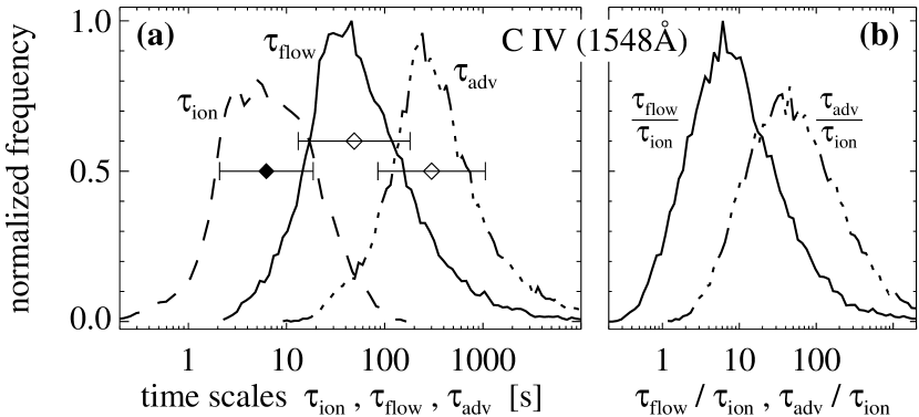
Figure 2.— The left panel (a) shows a histogram of ionization times $\tau_{\rm{ion}}$ for C³⁺ (dashed) as compared to histograms of flow times $\tau_{\rm{flow}}$ (solid) and advective times $\tau_{\rm{adv}}$ (dashed-dotted) at the temperatures where C IV (1548 Å) is formed. The diamonds show the median values of the respective times and the bars indicate the standard deviations.
The right panel (b) shows the histograms of the ratios of flow to ionization time, $\tau_{\rm{flow}}/\tau_{\rm{ion}}$ (solid), and advective to ionization time, $\tau_{\rm{adv}}/\tau_{\rm{ion}}$ (dashed-dotted). See Sect. 4.2.

Figure 3.— Comparison of time scales for ionization, flow and advection. The diamonds show the median values of the ionization time $\tau_{\rm{ion}}$ of the respective lines (standard deviation shown as bars, cf. 2a). The solid line shows the median flow time $\tau_{\rm{flow}}$ at the respective temperature in the MHD model. The dotted lines indicate the standard deviation of $\tau_{\rm{flow}}$. In addition the dashed-dotted line shows the median values of the advective times $\tau_{\rm{adv}}$. See Sect. 4.2.

4.2.2 Dynamic times

We use two procedures to determine a dynamic time, the first closer linked to the picture of particles getting ionized while flowing up a temperature gradient, the second more formally bound to the advective term in the rate equations.

The flow time $\tau_{\rm{flow}}$ we define as the time needed for a test particle with velocity $v$ to cross a given temperature difference $(\Delta\log{T})_{\rm{ion}}$. Thus within the time $\tau_{\rm{flow}}$ we put the test particle to a higher temperature and ask if the particle is ionized after this time. If this is not the case, i.e. if $\tau_{\rm{flow}}>\tau_{\rm{ion}}$, ionization equilibrium is a good approximation.

We choose a value of $(\Delta\log{T})_{\rm{ion}}=0.1$, as this is about the half width at half maximum of the contribution function for the emission lines (FWHM/2 in Table 1). When moving an ion by such a temperature difference it just starts “seeing” another ionization equilibrium.

Thus the inverse of the flow time is given by

$$\frac{1}{\tau_{\rm{flow}}}~{}=~{}\frac{{\nabla}(\log{T})\cdot\mbox{\boldmath$\hat{v}$\unboldmath}}{(\Delta\log{T})_{\rm{ion}}}~{}|\mbox{\boldmath$v$\unboldmath}|~{},$$ (17)

where the temperature gradient and the velocity vector $v$ are taken from the MHD model. $\hat{v}$ is the unit vector along $v$. The temperature gradient is projected on the flow direction as we are interested only in changes along the path of the test particle. Furthermore we consider only locations where the flow is in the direction of increasing temperature as only this will be affected by the ionization processes.

Like for the ionization times we now compute the distribution of flow times in each line formation region. These histograms can be directly compared to those of the ionization times, as it is done in 2a for C IV. This shows that for C IV the flow time is larger than the ionization time, which is also confirmed by the histogram of ratios of flow to ionization times (2b).

In 3 the median values of the flow times, $\tau_{\rm{flow}}$, are shown also for other temperatures in the MHD model as a solid line. The dotted lines indicate the standard deviation of $\tau_{\rm{flow}}$. As expected the flow time is smallest in the middle transition region below $10^{5}$ K as there the temperature gradient is steepest. $\tau_{\rm{flow}}$ increases by almost two orders of magnitude towards the corona as well as to the chromosphere. One should note that the absolute values of the flow times depend on the choice of $(\Delta\log{T})_{\rm{ion}}$.

A more direct way to compute a dynamic time is to evaluate the left-hand-side of the rate equations (15).

If considering only the process of electron collisional ionization for a single ionization state, the rate equation (15) reads

$$\frac{1}{n}~{}\frac{{\rm{d}}n}{{\rm{d}}t}+\frac{1}{n}~{}\nabla\cdot(n\,\mbox{\boldmath$v$\unboldmath})=-n_{e}~{}C_{\rm{ion}}~{},$$ (18)

with $n_{i}=n$ being the density of the respective ion, $n_{j}=n_{e}$ the electron density and $\gamma_{ij}=n_{i}\,n_{e}\,C_{\rm{ion}}$ the ionization rate. The right-hand side is the inverse ionization time as used in (16) and from the left-hand-side we can define an advective time scale

$$\frac{1}{\tau_{\rm{adv}}}~{}=~{}\frac{1}{n}~{}|\nabla\cdot(n\,\mbox{\boldmath$v$\unboldmath})|~{},$$ (19)

The divergence of the particle flux density $\nabla\cdot(n\,\mbox{\boldmath$v$\unboldmath})$ is calculated from the MHD model. Just like for $\tau_{\rm{flow}}$ we have computed the median values of $\tau_{\rm{adv}}$ and over-plotted them in 3 as a dashed-dotted line. At all temperatures the advective time scale is at least as large as the flow time scale defined above, $\tau_{\rm{adv}}>\tau_{\rm{flow}}$.

4.2.3 Comparing ionization and dynamic times

A comparison of the ionization time $\tau_{\rm{ion}}$ with the dynamic times $\tau_{\rm{flow}}$ and $\tau_{\rm{adv}}$ shows that in general the assumption of ionization equilibrium is satisfied in the model under investigation here.

A more detailed comparison of the distribution of ionization and dynamic times shows that there are regions where one definitely should not use ionization equilibrium. Mostly, like for C IV only a small fraction of the volume has flow times smaller than ionisation times (cf. in 2b only a minority has values of $\tau_{\rm{flow}}/\tau_{\rm{ion}}{<}1$). In our study it is only for C III and Si IV that the assumption of ionisation equilibrium is violated in the sense that $\tau_{\rm{flow}}{<}\tau_{\rm{ion}}$, but even then the ionisation time is still smaller (or comparable) to the the advection time $\tau_{\rm{adv}}$ (cf. 3).

From this we can conclude that for the present work and as a first step for a spectroscopic analysis of complex 3D MHD coronal models we might well use ionization equilibrium. Future work, however, should try to include also non-equilibrium effects.

4.2.4 Ionization equilibrium and flows

It is often argued that departures from the ionization equilibrium become of vital importance as soon as the velocities across a temperature gradient become “large enough”. As shown in the preceding subsection in our computation the ionization times are (generally) still shorter than the time scales of the flows, and hence the assumption of ionization equilibrium is not too bad.

This is in contrast to earlier considerations, e.g. of Joselyn et al. (1979), who argued that velocities of the order of 10 km/s will certainly lead to a violation of ionization equilibrium. They used the temperature gradients from static models (e.g. Gabriel, 1976) to calculate time scales of the plasma flowing across these temperature gradients. However, such an analysis does not account for the back reaction of the flow on the temperature gradient, and thus a too small time scale is derived.

Figure 4.— Average temperature gradient along the streamlines in the MHD model underlying the present analysis as a function of temperature for regions with flow speeds of about 10  km/s (dashed) and 0.5 km/s (solid). For comparison the gradient in the static model of Gabriel (1976) is shown as a dot-dashed line. The bar represents the scatter of gradients in each temperature bin. See Sect. 4.2.4.

To illustrate this we plot the average temperature gradient (along streamlines) as a function of temperature within the box of the MHD model, once for only those regions with velocities of about 10 km/s (dashed) and about 0.5 km/s (solid) in 4. It is clearly evident that the temperature gradient is smaller in regions with higher velocities. For comparison we plot the temperature gradient in a static coronal (funnel) model (dot-dashed in 4; Gabriel, 1976). In the case of small velocities the temperature gradient in the MHD model underlying the present analysis is almost as steep as in a static model (factor $\sim$2 in the middle transition region). As there is no heating in the transition region of the static model of Gabriel (1976), while in the 3D MHD model with flux-braiding the heating is strongly concentrated at low heights, one expects this somewhat shallower gradient in the latter case. The main point to stress here is that if the flow speed is larger, the gradient becomes much flatter, by about an order of magnitude, as the flow is smoothing the temperature gradient (cf. solid and dashed line in 4).

From this discussion one might draw the following conclusion. For a higher velocity the temperature gradient will decrease, which partly compensates the effect of a faster speed when calculating the flow time using e.g. (17). By this the back reaction of the flow on the temperature helps in simplifying the treatment of ionization to the case of equilibrium. However, for models with more violent flows, the assumption of ionization equilibrium certainly will break down.

4.3. DEM from the MHD calculations

To check the validity of the inversion of the differential emission measure (DEM) discussed in Sect. 3.3 we calculate the DEM directly from the MHD results, i.e. the density. For a traditional DEM inversion one has to assume a 1D atmosphere with a monotonic increase in temperature. Only then the DEM definition in (14) makes sense. However, this is not the case in a highly structured atmosphere as under investigation here. Thus we start by defining a volume emission measure

$${{\rm{EM}}}_{V}\,(T)~{}=~{}\int_{V}n_{e}^{2}~{}{\rm{d}}V~{},$$ (20)

where the integration is over a volume typically contributing to an emission line formed at temperature $T$. According to the contribution functions to the line (Sect. 4.1) the volume covers a temperature interval of ${\pm}0.15$ in ${\log}T$, i.e. ${\Delta}{\log}T{=}0.3$.

To move to a height-related expression the volumetric emission measure is divided by the area $A$ of the box giving an average column emission measure ${{\rm{EM}}}_{h}={{\rm{EM}}}_{V}/A$. Now one can formally substitute the volume integration by a height integration ${\rm{d}}h={\rm{d}}V/A$ and this by an integration over temperature,

$${{\rm{EM}}}_{h}=\int_{h}n_{e}^{2}~{}{\rm{d}}h\quad\Leftrightarrow\quad{{\rm{EM}}}_{h}=\int n_{e}^{2}~{}\frac{{\rm{d}}h}{{\rm{d}}T}~{}{\rm{d}}T~{}.$$ (21)

Using the definition of the DEM (14) one gets

$${{\rm{EM}}}_{h}=\int{{\rm{DEM}}}~{}{\rm{d}}T~{}.$$ (22)

Thus one can approximate the DEM by

$${{\rm{DEM}}}_{\rm{MHD}}~{}=~{}\frac{{{\rm{EM}}}_{h}}{\Delta T}~{}=~{}\frac{{{\rm{EM}}}_{V}}{A\,\Delta T}~{},$$ (23)

where ${\Delta}T$ is the temperature range corresponding to ${\Delta}{\log}T{=}0.3$, i.e. ${\Delta}T$ increases with temperature.

Using (20) this allows the calculation of the ${{\rm{DEM}}}$ directly from the MHD model, which can be compared to the ${{\rm{DEM}}}$ as resulting from the inversion of line intensities as outlined in Sect. 3.3.

In 9 we plot the DEM derived directly from the MHD model as following (23) as a dot-dashed line along with the DEM from the inversion using the line emissivities (solid) as discussed in Sect. 3.3. We see that they compare relatively well, even though the difference at high temperatures is noticeable. As this discrepancy is probably (at least partly) due to the highly structured nature of the atmosphere, a further discussion is shifted to Sect. 5.5.

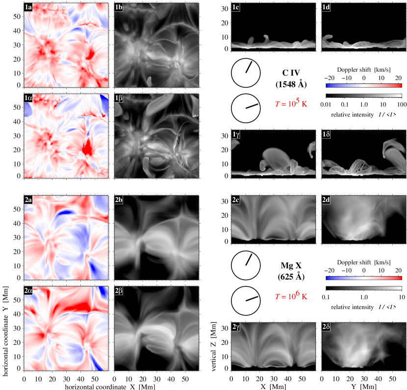
Figure 5.— Spatial maps in Doppler shift and intensity in the lines of C IV (1548 Å) and Mg X (625 Å) formed at about $10^{5}$ and $10^{6}$ K, respectively, for two different time steps of the MHD model about 7 minutes apart (at $t{=}4$  min and 11 min).
The two top panels labeled with 1 show C IV, the two bottom panels labeled with 2 show Mg X. The maps of the earlier time step are labeled with Latin letters (1st and 3rd row), those for the time step 7 minutes later with Greek letters (2nd and 4th row).
The panels (a/$\alpha$) show the Doppler shift of the synthesized spectra as seen from straight above, the panels (b/$\beta$) show the same for the intensity of the respective line. This corresponds to the appearance near disk center. Panels (c/$\gamma$) and (d/$\delta$) show side views of the computational box along the x and y axis in line intensity, which resembles the appearance at the limb.
The intensities $I$ are scaled with respect to the average (median) intensity $\langle{I}\rangle$ of the respective map.

5. Results

Here we will only give some examples of the results that may be achieved using the spectroscopic analysis described in this paper. More specific problems, such as time variability, evolution or spatial structure will be addressed in future investigations and will provide new tests for the model of coronal heating through flux braiding.

5.1. Morphology: intensity and Doppler shift maps

By investigating maps in intensity and Doppler shift in various lines when integrating along a line-of-sight through the box, one can now study the morphology of the transition region and corona. Such maps are provided in 5 for C IV formed in the low transition region at ${\sim}10^{5}$ K (top rows labeled with 1) and for Mg X formed in the low corona at ${\sim}10^{6}$ K (bottom rows labeled with 2). There the respective leftmost panels (a/$\alpha$) show the Doppler maps when looking from straight above and the panels b/$\beta$ show the same in intensity — this would correspond to an observation at disk center. The right panels (c/$\gamma$, d/$\delta$) show intensity maps when looking from the sides at the box (displayed with correct horizontal/vertical aspect ratio) — this corresponds to the appearance at the limb. For each line the snapshots at two times are shown at some 4 and 11 minutes into the simulation (labeled by Latin and Greek letters, respectively).

In an earlier publication we reported shortly on the more structured appearance of the transition region being due to heat conduction and the numerous structures in coronal Doppler shifts (Peter et al., 2004).

When comparing the intensity maps of the two time steps only seven minutes apart, it is striking how much the transition region has changed in this time, while the corona still looks pretty much the same in intensity. This is of special interest, if one recalls that the driver of the corona, the photospheric granular motion, acts on the time scale of some 5 to 10 minutes. Thus the transition region directly responds to the changes in the photospheric magnetic structure, while the corona is reacting much slower. This difference is mainly due to the large difference in cooling time scale and the very efficient re-distribution of energy trough heat conduction at high temperatures.

Not surprisingly also the Doppler map of the transition region changes significantly during the only seven minutes on small scales. Despite the smooth, slowly-evolving appearance in intensity, the corona reveals its dynamic structure in the Doppler map. While the heat conduction quickly distributes the deposited energy, still the dynamic response of the plasma to the heating process is present, showing up as flows causing the Doppler shifts. And just like in the transition region, the coronal Doppler shifts show large variations on small spatial scales within the time scale of the photospheric driver.

This high variability of the coronal Doppler maps shows the need to study coronal variations on short time scales not only using intensity maps like provided by EIT/SOHO or TRACE. If one could obtain Doppler maps with high temporal resolution, one would have access to the dynamic response of the corona to the heating process, which is not available through intensity maps alone. Unfortunately current slit spectrographs like SUMER or CDS on SOHO do not provide maps of sufficient size in a reasonable time cadence.

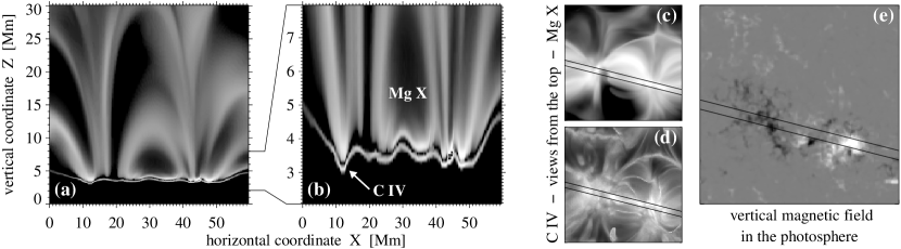
Figure 6.— Composite view of a thin vertical slice of the computational box in C IV (${\sim}10^{5}$ K) and Mg X (${\sim}10^{6}$ K) at time $t{=}4$ min. The left panel (a) shows the vertical slice as defined by the black lines in the top views (c,d) when integrating along the Y direction; actually panels (c,d) are the same as panels (1b,2b) of 5.  The location of the slice with respect to the photospheric magnetic field map is shown in panel (e). The middle panel (b) shows part of panel (a) stretching the vertical axis to highlight the structure in the low parts of the atmosphere. The emission as seen in C IV and Mg X comes from disjunct areas of the vertical slice. The lower “line” shows the emission from C IV, while the upper more diffuse emission stems completely from Mg X. See Sect. 5.2.

5.2. Vertical structure: roiling and loops

To show the further potential of the forward modeling technique presented here, we investigate a vertical slice of the computational box cutting the two main polarities forming the active region. In 6 c, d, and e we show the location (between the lines) of the vertical slice in the horizontal plane for the intensity maps in C IV and Mg X as well as the photospheric magnetogram. The left panel (6a) shows the vertical slice, the emission from C IV and Mg X displayed on top of each other. Please note that in contrast to 5 here the aspect ratio is not unity, but about a factor of two.

The emission from these two lines comes from practically disjunct regions. The coronal Mg X emission stems from the diffuse loop-dominated part in the upper part of the image, while the transition region C IV emission originates from a very thin layer below the corona. Panel b of 6 shows the area from ${\sim}2$–$8$ Mm height vertically stretched to show the transition region more clearly. At least in this region the transition region emission comes from an area below the coronal source region, i.e. from the footpoint regions of the coronal magnetic structures.

6b also reveals that the transition region is roiling field, while being very thin in the vertical direction (some 100 km). This is to be expected, as the heating is highly variable in space and time and thus the location of the transition region is to be expected to move up and down to adjust the coronal pressure in accordance with the heating rate. This is well known from 1D loop models (e.g. Hansteen, 1993) and also commented on by Gudiksen & Nordlund (2005a). Despite being very thin, the roiling of the transition region leads to a relatively thick appearance when integrating along a horizontal direction. In 6b the roiling of the transition region has an amplitude in height of about 1 Mm or more, while at other places and times it can be even more. Thus the roiling leads to a transition region that would appear several Mm thick when observed at the limb, as nicely illustrated by the side views in 5, panels 1c and 1d. This corresponds well will observations of limb intensity profiles at the limb (e.g. Mariska et al., 1978).

5.3. Average line shifts

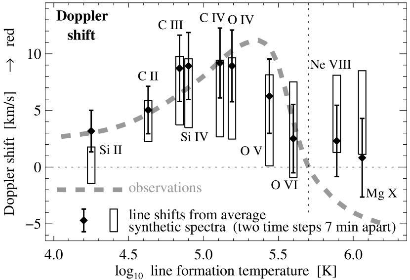
Figure 7.— Comparison of synthesized and observed Doppler shifts for two time steps about 7 minutes apart (same times as in 5; $t{=}4,11$ min). The diamonds show the Doppler shifts of the average spectra and the bars indicate the standard deviation of the Doppler shifts of a spatial map as seen looking from straight above on the computational box for the earlier time step. The rectangles show the same but for 7 minutes later. The change in this short time is noticeable. The lines are plotted at the formation temperature as following from the contribution to the emission from the present work (cf. Table 1). The thick dashed line shows the trend as found in observations. See Sect. 5.3.

The time-average of the line shifts derived from the synthetic corona presented here were discussed previously (Peter et al., 2004). In 7 we plot the average line shifts as a function of line formation temperature for the two individual time steps, seven minutes apart, which have been displayed also in the spatial maps in 5. The Doppler shifts are calculated for a vertical line-of-sight, i.e. when looking at the computational box from straight above. The height of the bars and rectangles represents the spatial scatter for each time step (1/2 of the standard deviation). The trend found in observations is plotted as a thick dashed line (compiled from Brekke et al., 1997; Chae et al., 1998b; Peter & Judge, 1999).

It is obvious that the average Doppler shifts change quite dramatically, and the overall shape varies from being very close to the observations (bars) to a more flat profile with comparable Doppler shifts at all temperatures (rectangles) — and this happening in only seven minutes. The time variation of the Doppler shift for some 20 minutes is shown in 10b for a number of lines. Here we see that for all lines, also for the coronal Mg X line, the variation over these 20 minutes is comparable or larger than the spatial scatter in the data. This again emphasizes the potential provided by observations of Doppler shifts throughout the outer solar atmosphere, as pointed out at the end of Sect. 5.1.

In the present model the persistent redshifts in the transition region, puzzling theorists since their discovery by Doschek et al. (1976), are caused by the flows induced by the heating through braiding of magnetic flux. Being free of spurious assumptions, this is the first time one finds an explanation of the Doppler shifts providing a qualitative and quantitative representation of the redshifts in the middle transition region. The blue shifts towards higher temperatures are not matched yet, but we see a clear indication that above $\log{T}{\approx}5.2$ the redshifts are decreasing, and at some periods of time in the model run, we are quite close to the observations (cf. bars in 7). Further investigations, especially with an improved upper boundary condition or a larger box, will have to address this discrepancy.

5.4. Average non-thermal line widths

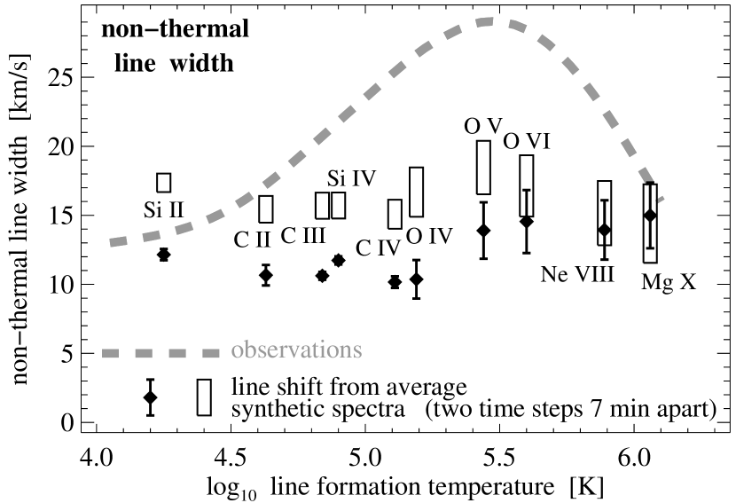
Figure 8.— Comparison of synthesized and observed non-thermal widths. Similar as 7 but now for non-thermal widths. See Sect. 5.4.

Another important test for any coronal model is provided by a comparison of the non-thermal line widths. These contain information on the non-thermal unresolved motions, introduced by the limited resolution in space and time of any instrument. Averaging in space and time will mix spectral information with different velocities and will lead to a broadening of the line. It is important to note that also the integration along the line-of-sight contributes to the non-thermal broadening, and there is (almost) nothing we can do about this from an observers point of view.

In 8 we plot the non-thermal line width of the average spectrum for the two time steps seven minutes apart already displayed in 5 and 7 (again when looking at the computational box from straight above). The thick dashed line shows the trend in observations compiled from Chae et al. (1998a) and Peter (2001).

In the corona and the low transition region the non-thermal width from the synthesized spectra match roughly the observed values, but in the middle transition region the synthetic spectra show significantly smaller widths than the observations. There is (at least) one possible explanation for this. The high non-thermal broadening observed on the Sun might be due to small scale velocities connected with the heating process itself, i.e. the nano-flares induced by the flux-braiding. And this effect is to be expected to have the largest effect in the middle transition region, where the time scales are shortest. Because of their tiny spatial scale, these nano-flares cannot be modeled in the MHD simulation, which the spectral synthesis is based upon. Future models with increased spatial resolution will have to show if this mismatch with the observations can be resolved.

5.5. What do we learn from the differential emission measure?

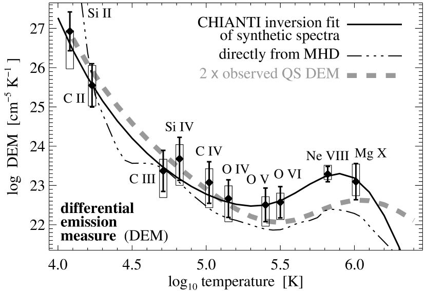
Figure 9.— Comparison of the differential emission measure (DEM) as derived from the synthesized and observed spectra. The solid line shows the fit from the DEM inversion based on the synthesized lines displayed as bars (Sect. 3.3; for time $t{=}4$ min). The lines are displayed here at the formation temperature as following from the DEM inversion (cf. Table 1). This differs slightly from the temperatures used in Figs. 7 and 8. The rectangles show the situation about 7 minutes later at $t{=}11$ min, the changes being very small. The thick dashed line is based on a DEM inversion using observed quiet Sun disk center line radiances observed with SUMER, scaled by a factor of two. The dot-dashed line displays the DEM curve as following directly from the MHD results (Sect. 4.3). See Sect. 5.5.

As outlined in Sect. 3.3 and 4.3, we perform an differential emission measure (DEM) analysis using the spectral lines listed in Table 1 using the atomic data package CHIANTI. The resulting DEM curve for one single time step (at 4 minutes into the simulation) is plotted in 9 as a solid line. The diamonds show the DEM at the line formation temperature of the respective line, multiplied by the ratio of the observed emissivity to the one predicted by the DEM fit. Thus the displacement of the diamonds from the solid line represent the error of the DEM fit. The height of the bars represent the scatter of the emissivities.

As we discussed previously (Peter et al., 2004) this is the first model to reproduce the overall shape of the DEM curve quantitatively and qualitatively, especially the increase of the DEM towards lower temperatures below $\log{}T{=}5.3$. For comparison we plotted an DEM inversion based on radiance data at disk center taken from Wilhelm et al. (1998), for Mg X and Si II we re-evaluated some SUMER disk center spectra. The agreement is remarkable, except for the highest temperatures. This discrepancy is partly due to a lack of constraining lines at higher temperatures, as the maximum temperature in the MHD simulation is about $\log{T}{\approx}6.3$. Thus the DEM inversion is not very well defined at high temperatures. This becomes especially important when discussing the temporal variability of the DEM below.

The DEM inversion based on the synthesized spectra roughly agrees with the DEM derived directly from the MHD models (cf. Sect. 4.3). While for the DEM inversion one implicitly assumes a simple 1D stratified static atmosphere (cf. Sect. 3.3) this is certainly not the case in the computational box. In this light it is even surprising that the DEM derived directly from the MHD model (9, dot-dashed line) roughly compares to the inversion, especially below $\log{T}{=}5.0$.

In 9 the rectangles represent the situation concerning the DEM inversion 7 minutes after the time step discussed so far (represented by the bars). The change is very small. This is emphasized by the temporal evolution of the DEM inversion fit at temperatures representing the low and middle transition region as well as the low corona (10a). It is clearly evident that the changes in the DEM fit are only very small. At $\log{T}{=}5.9$ the fit is “jumping”, as the DEM inversion is not well constrained at high temperatures (see above). Thus also the jump of the fit for $\log{T}{=}5.9$ at time ${\sim}18$ minutes is an artefact and not real.

Figure 10.— Temporal evolution of the differential emission measure (DEM) and the average Doppler shift. The top panel (a) shows the evolution for the DEM at three different temperatures as following from DEM inversion fits like the one shown in 9. The bottom panel (b) shows the variation of the Doppler shifts for emission lines spanning temperatures from $\log{T}{\sim}4.6$ to $6.0$. Please note that the variation in DEM in much smaller than the uncertainties (represented by the bars in both panels) and is thus not significant. In contrast, the variation in Doppler shift is significant. The Figs. 5 – 9 show snapshots at $t{=}4$ min and 11 min. See Sect. 5.5.

The important result here is that the DEM hardly changes with time (over the 20 minutes of the simulation), but within the uncertainties stays constant. This is in strong contrast to the Doppler shifts, which change significantly at all temperatures.

The DEM curve thus provides an important test for a coronal heating model, in particular in the sense that it is not easy to get the overall shape right. However, once one gets the overall shape right, it seems that the DEM stays fixed, and therefore provides only limited potential for further diagnostics of the structure and dynamics of the coronal heating process.

6. Conclusions

We have presented a procedure how to synthesize EUV spectra from a complex 3D MHD model for a stellar corona, in which the heating is due to flux braiding through photospheric footpoint motions. An investigation of the validity of the ionization equilibrium showed that in the present case this simplification is justified. Because the heating is concentrated very low in the atmosphere, the temperature gradients are much shallower than in traditional static models, and thus the typical dynamic (or flow) times are larger than the ionization times. However, for models with more violent flows one will have to properly solve the ionization rate equations. We found that due to the strong heating at the footpoints of the corona and the resulting strong increase of density towards the chromosphere, cool lines like from Si II tend to be formed well below their ionization equilibrium temperature. Thus the cool lines are of limited diagnostic value for the transition region.

Together with the spectral synthesis the MHD simulation provides a forward model, which allows a direct comparison to observations, and by this is a powerful tool to investigate the corona. In this paper we describe some of the potentials of this method.

The spatial maps of intensity show a much higher spatial and temporal variability in the transition region than in the corona. In the transition region the temporal variability occurs on a time scale compatible with the photospheric driver of the coronal heating. In the Doppler shift maps, however, the spatial variability is also very large in the corona, much stronger than the variability in intensity. This shows the need for further instrumentation to get access to coronal Doppler maps with sufficient temporal resolution (below 5 minutes).

Likewise the time variation of the Doppler shifts is significant, while the differential emission measure (DEM), derived from the intensities, shows only a very small variation. While this model is the first to reproduce qualitatively and quantitatively the form of the DEM variation with temperature, it also shows the limitations of the DEM analysis in a highly dynamic atmosphere. To understand the dynamics of the corona it is vital to use the Doppler shifts as a crucial test for the model, and not only the line intensity or emission measures.

This study shows the pivotal importance of forward modeling for our understanding of stellar coronae, as it provides numerous controllable ways to compare model results and observations.

References

- Arnaud & Rothenflug (1985) Arnaud, M. & Rothenflug, R. 1985, A&AS, 60, 425
- Brekke et al. (1997) Brekke, P., Hassler, D. M., & Wilhelm, K. 1997, Sol. Phys., 175, 349
- Brković et al. (2003) Brković, A., Peter, H., & Solanki, S. K. 2003, A&A, 403, 725
- Chae et al. (1998a) Chae, J., Schühle, U., & Lemaire, P. 1998a, ApJ, 505, 957
- Chae et al. (1998b) Chae, J., Yun, H. S., & Poland, A. I. 1998b, ApJS, 114, 151
- Del Zanna et al. (2002) Del Zanna, G., Landini, M., & Mason, H. E. 2002, A&A, 385, 968
- Dere et al. (1997) Dere, K. P., Landi, E., Mason, H. E., Monsignori Fossi, B. C., & Young, P. R. 1997, A&AS, 125, 149
- Doschek et al. (1976) Doschek, G. A., Feldman, U., & Bohlin, J. D. 1976, ApJ, 205, L177
- Dowdy et al. (1986) Dowdy, J. F., Rabin, D., & Moore, R. L. 1986, Sol. Phys., 105, 35
- Edlén (1942) Edlén, B. 1942, Zeitschrift f. Astrophys., 22, 30
- Gabriel (1976) Gabriel, A. H. 1976, Phil. Trans. Roy. Soc. Lond., A 281, 339
- Galsgaard & Nordlund (1996) Galsgaard, K. & Nordlund, Å. 1996, J. Geophys. Res., 101, 13445
- Grotrian (1939) Grotrian, W. 1939, Naturwiss., 27, 214
- Gudiksen & Nordlund (2002) Gudiksen, B. & Nordlund, Å. 2002, ApJ, 572, L113
- Gudiksen & Nordlund (2005a) —. 2005a, ApJ, 618, 1020
- Gudiksen & Nordlund (2005b) —. 2005b, ApJ, 618, 1031
- Hansteen (1993) Hansteen, V. H. 1993, ApJ, 402, 741
- Hendrix et al. (1996) Hendrix, D. L., van Hoven, G., Mikic, Z., & Schnack, D. D. 1996, ApJ, 470, 1192
- Joselyn et al. (1979) Joselyn, J., Munro, R. H., & Holzer, T. E. 1979, Sol. Phys., 64, 57
- Judge & McIntosh (1999) Judge, P. G. & McIntosh, S. W. 1999, Sol. Phys., 190, 331
- Landini & Monsignori Fossi (1990) Landini, M. & Monsignori Fossi, B. C. 1990, A&AS, 82, 229
- Mariska et al. (1978) Mariska, J. T., Feldman, U., & Doschek, G. A. 1978, ApJ, 226, 698
- Mazzotta et al. (1998) Mazzotta, P., Mazzitelli, G., Colafrancesco, S., & Vittorio, N. 1998, A&AS, 133, 403
- McIntosh (2000) McIntosh, S. W. 2000, ApJ, 533, 1043
- Müller et al. (2004) Müller, D., Peter, H., & Hansteen, V. H. 2004, A&A, 424, 289
- Okabe et al. (1992) Okabe, A., Boots, B., & Sugihara, K. 1992, Spatial tessellations. Concepts and applications of voronoi diagrams (Wiley Series in Probability and Mathematical Statistics, Chichester, New York)
- Parker (1972) Parker, E. N. 1972, ApJ, 174, 499
- Peter (1999) Peter, H. 1999, ApJ, 516, 490
- Peter (2001) —. 2001, A&A, 374, 1108
- Peter et al. (2004) Peter, H., Gudiksen, B., & Nordlund, Å. 2004, ApJ, 617, L85
- Peter & Judge (1999) Peter, H. & Judge, P. G. 1999, ApJ, 522, 1148
- Priest et al. (1998) Priest, E. R. et al. 1998, Nature, 393, 545
- Reeves (1976) Reeves, E. M. 1976, Sol. Phys., 46, 53
- Roussev et al. (2001) Roussev, I., Doyle, J. G.and Galsgaard, K., & Erdélyi, R. 2001, A&A, 380, 719
- Roussev & Galsgaard (2002) Roussev, I. & Galsgaard, K. 2002, A&A, 697–705
- Spitzer (1956) Spitzer, L. 1956, Physics of fully ionized gases (Interscience, New York)
- Ulmschneider et al. (1991) Ulmschneider, P., Priest, E. R., & Rosner, R., eds. 1991, Mechanisms of chromospheric and coronal heating (Springer-Verlag, Berlin)
- von Steiger et al. (2000) von Steiger, R., Schwadron, N. A., Fisk, L. A., et al. 2000, J. Geophys. Res., 105(A12), 27217
- Walsh et al. (2004) Walsh, R., Ireland, J., Danesy, D., & Fleck, B., eds. 2004, Coronal Heating — Proceedings of the SOHO 15 workshop, ESA SP-575 (European Space Agency, Paris)
- Wikstøl et al. (1998) Wikstøl, Ø., Judge, P. G., & Hansteen, V. H. 1998, ApJ, 501, 895
- Wilhelm et al. (1995) Wilhelm, K., Curdt, W., Marsch, E., et al. 1995, Sol. Phys., 162, 189
- Wilhelm et al. (1997) Wilhelm, K., Lemaire, P., Curdt, W., et al. 1997, Sol. Phys., 170, 75
- Wilhelm et al. (1998) Wilhelm, K., Lemaire, P., Dammasch, I. E., et al. 1998, A&A, 334, 685
- Withbroe & Noyes (1977) Withbroe, G. L. & Noyes, R. W. 1977, ARA&A, 15, 363
- Young et al. (2003) Young, P. R., Del Zanna, G., Landi, E., Dere, K. P., Mason, H. E., & Landini, M. 2003, ApJS, 144, 135