Is the ‘IR Coincidence’ Just That?

Abstract

Previous work by Motch et al. (1985) suggested that in the low/hard state of GX 339$-$4 the soft X-ray power-law extrapolated backward in energy agrees with the IR flux level. Corbel & Fender (2002) later showed that the typical hard state radio power-law extrapolated forward in energy meets the backward extrapolated X-ray power-law at an IR spectral break, which was explicitly observed twice in GX 339$-$4. This ‘IR coincidence’ has been cited as further evidence that synchrotron radiation from a jet might make a significant contribution to the observed X-rays in hard state black hole systems. We quantitatively explore this hypothesis with a series of simultaneous radio/X-ray observations of GX 339$-$4, taken during its 1997, 1999, and 2002 hard states. We fit these spectra, in detector space, with a simple, but remarkably successful, doubly broken power-law model that indeed requires an IR spectral break. For these observations, the break position and the integrated radio/IR flux have stronger dependences upon the X-ray flux than the simplest jet model predictions. If one allows for a softening of the X-ray power law with increasing flux, then the jet model can agree with the observed correlation. We also find evidence that the radio flux/X-ray flux correlation previously observed in the 1997 and 1999 GX 339$-$4 hard states shows a ‘parallel track’ for the 2002 hard state. The slope of the 2002 correlation is consistent with observations taken in prior hard states; however, the radio amplitude is reduced. We then examine the radio flux/X-ray flux correlation in Cyg X-1 through the use of 15 GHz radio data, obtained with the Ryle radio telescope, and Rossi X-ray Timing Explorer data, from the All Sky Monitor and pointed observations. We again find evidence of ‘parallel tracks’, and here they are associated with ‘failed transitions’ to, or the beginning of a transition to, the soft state. We also find that for Cyg X-1 the radio flux is more fundamentally correlated with the hard, rather than the soft, X-ray flux.

1. Introduction

Both Cyg X-1 and GX 339$-$4 in their spectrally hard, radio-loud states have served as canonical examples of the so-called ‘low state’ (or ‘hard state’) of galactic black hole candidates (see Pottschmidt et al. 2003; Nowak et al. 2002, and references therein). As we discuss below, in this state the X-ray spectrum is reasonably well-approximated by a power-law with photon spectral index (i.e., photon flux per unity energy $\propto E^{-\Gamma}$) of $\Gamma\approx 1.7$, with the power-law being exponentially cutoff at high energies ($\approx 100$ keV). It long has been suggested that such spectra are due to Comptonization of soft photons from an accretion disk by a hot corona in the central regions of the compact object system (e.g., Sunyaev & Trümper 1979). Comptonization models have been very successful in describing the broad-band X-ray/soft gamma-ray spectra of both Cyg X-1 (Pottschmidt et al. 2003) and GX 339$-$4 (Nowak et al. 2002).

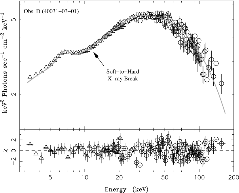
Figure 1.— Left: Unfolded spectra of a simultaneous radio and X-ray spectrum of GX 339$-$4 (D, Observation ID 40031-03-01, in Tables 1 and 2), fit with an absorbed, exponentially cutoff, doubly broken power-law and a gaussian line. Residuals are from the proper forward folded model fit. Right: Same unfolded spectrum as on the left, showing just the RXTE data.

It recently has been hypothesized, however, that the X-ray spectra of hard state sources might instead be due to synchrotron and synchrotron self-Compton (SSC) radiation from a mildly relativistic jet (Markoff et al. 2001, 2003). Jet models have been prompted in part by multi-wavelength (radio, optical, X-ray) observations of hard state systems. Although radio emission from Cyg X-1 was first observed quite some time ago (Braes & Miley 1971), it is more recently that a radio jet has been imaged (Stirling et al. 2001), and that the low/hard state X-ray flux has been shown to be positively correlated with the radio flux (Pooley et al. 1998).

Radio emission also has been discovered in GX 339$-$4 (Sood & Campell-Wilson 1994). The radio emission is correlated with X-ray flux in spectrally hard states (Hannikainen et al. 1998), but is quenched during spectrally soft states (Fender et al. 1999). Furthermore, in hard states of GX 339$-$4, the 3–9 keV X-ray flux (in units of $10^{-10}~{}{\rm erg~{}cm^{-2}~{}s^{-1}}$) is related to the 8.6 GHz radio flux (in mJy) by ${F_{\rm x}}\approx 0.46{\cal F}_{\rm r}^{1.42}$ (Corbel et al. 2003, noting that throughout this paper we shall use caligraphic script to denote flux densities, i.e., flux per unit energy, and roman script to denote flux integrated over an energy band). This correlation was seen to hold over several decades in X-ray flux, and also to hold for two hard state epochs that were separated by a prolonged, intervening soft state outburst. Similar correlations were found between energy bands in the 9–200 keV range and the radio flux (Corbel et al. 2003). It further has been suggested that the ${F_{\rm x}}\propto{\cal F}_{\rm r}^{1.4}$ correlation is a universal property of the low/hard state of black hole binaries (Gallo et al. 2003).

This specific power-law dependence of the radio flux upon the X-ray flux naturally arises in synchrotron jet models (Falcke & Biermann 1995; Corbel et al. 2003; Markoff et al. 2003; Heinz & Sunyaev 2003). Both the location of the break from an optically thick to an optically thin radio spectrum (presumed to continue all the way through the X-ray), and the amplitude of the optically thick portion of the radio spectrum, vary with input power to the jet so as to produce the ${F_{\rm x}}\propto{\cal F}_{\rm r}^{1.4}$ scaling. Assuming, however, that the X-ray power of a disk/corona is proportional to $\dot{M}^{2}$, where $\dot{M}$ is the accretion rate, while the jet power is proportional to $\dot{M}$, also reproduces the scaling relationship (Markoff et al. 2003; Heinz & Sunyaev 2003; Fender et al. 2003; Merloni et al. 2003; Falcke et al. 2004).

Interestingly, nearly 20 years ago Motch et al. (1985) noted that for a set of simultaneous IR, optical, and X-ray observations of the GX 339$-$4 hard state, the extrapolation of the X-ray power-law to low energy agreed with the overall flux level of the optical/IR data. Corbel & Fender (2002) reanalyzed these observations, which did not include simultaneous radio data, as well as a set of (not strictly simultaneous) radio/IR/X-ray observations from the 1997 GX 339$-$4 hard state. They showed that the low energy extrapolation of the X-ray power-laws, and the high energy extrapolation of the radio power-law, coincided with a spectral break in the IR. The spectral shapes below and above the IR break were roughly consistent with the radio and X-ray power-laws, respectively. This ‘IR coincidence’ has been cited as further evidence that the jet not only accounts for the flat spectrum from radio through infrared, but also that optically thin emission from the jet, occurring at energies above the IR break, provides a significant contribution to the observed X-rays (Corbel & Fender 2002; Corbel et al. 2003; Markoff et al. 2003).

In this paper, we quantitatively examine the ‘IR coincidence’ with a series of simultaneous radio/X-ray spectra of GX 339$-$4. We use broken power-law fits to the combined radio and X-ray spectra to determine the extrapolated position of the break as a function of observed X-ray flux. We then reassess the correlation between radio and X-ray flux for GX 339$-$4 by including more recent hard state observations that occurred at fairly high X-ray fluxes. Based upon our results for GX 339$-$4, we also reassess this correlation for the case of Cyg X-1. We then summarize our results.

2. The ‘IR Coincidence’ in GX 339$-$4

2.1. Data Analysis

We consider a set of ten simultaneous radio/X-ray observations of GX 339$-$4, eight of which were discussed previously by us (Wilms et al. 1999; Nowak et al. 2002; Corbel et al. 2003) and come from the 1997 or 1999 hard state, and two of which were discussed by Homan et al. (2004) and come from the 2002 hard state (approximately a month before a soft state transition). All X-ray observations were performed with the Rossi X-ray Timing Explorer (RXTE). Their observation IDs and associated radio flux densities and integrated X-ray fluxes are presented in Table 1. Note that four of these observations are further labeled A–D, as we single these out for special discussion below. Observations A and B (40108-01-03 and 40108-01-04) occurred immediately after the 1999 soft-to-hard state transition (Nowak et al. 2002) and have optically thin radio spectra ($\alpha_{\rm r}<0$). Observation C and D (70109-01-02 and 40031-02-01) have the brightest X-ray fluxes in our sample, and are among the brightest hard X-ray states observed in GX 339$-$4 to date.

To analyze the X-ray spectra of these observations, RXTE response matrices were created using the software tools available in HEASOFT 5.3. The Proportional Counter Array (PCA) data were rebinned to have a minimum of 30 counts per bin, uniform systematic uncertainties of 0.5% were applied, and only data between 3 and 22 keV were considered. The High Energy X-ray Timing Explorer (HEXTE) data were coadded from the two individual clusters and then were rebinned to have a minimum signal-to-noise ratio (after background subtraction) of 10 in each bin. We considered HEXTE data only in the 18–200 keV range. In the fits discussed below, a multiplicative constant was allowed between the PCA and HEXTE normalization, with the PCA constant fixed to unity. The normalizations of the two instruments were always found to be the same to within a few percent (see Table 2).

The radio data for observation D (40031-03-01) were obtained with the Australia Telescope Compact Array (ATCA) at 4.8 GHz and 8.6 GHz. The radio data for observation C (70109-01-02) were also obtained with ATCA, but at 1.4 and 2.4 GHz. These radio data, as well as the data for observation B (40108-01-04), the 1999 April 22 observation (40108-02-02), and the 1999 May 14 observation (40108-02-03) have been reanalyzed by us. All other radio data come from Wilms et al. (1999), Nowak et al. (2002), and Corbel et al. (2000). In cases of small discrepancies between these latter references, we have adopted the radio flux values of Corbel et al. (2000), since, aside from the radio observations reanalyzed by us, that work represents the most up to date analysis of the radio data presented here.

Note that we have considered only data wherein we have nearly simultaneous radio and X-ray spectra. The radio/X-ray observations discussed by Nowak et al. (2002) all have a large degree of overlap between the radio and X-ray observing times, and they show very little long time scale ($>1000$ s) variability (Corbel et al. 2000). Radio observations C & D occur approximately a half day after their corresponding RXTE observations, but, again, neither the radio data nor the RXTE data show any evidence for long term variability within the observations themselves. Still, the lack of strict simultaneity might be a relevant factor in some of the results discussed below.

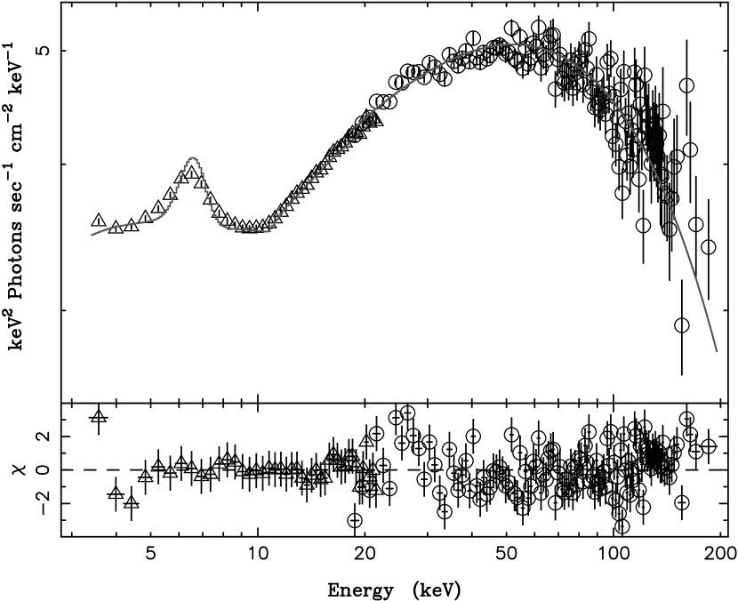
Figure 2.— Unfolded RXTE spectra of Cyg X-1 (Wilms et al., in prep.), fit with an absorbed, exponentially cutoff, broken power-law and a gaussian line. Residuals are from the proper forward folded model fit.

We further require that the source was bright enough to fit the X-ray spectrum in both the PCA and the HEXTE data. As discussed by Corbel et al. (2003) and Wardziński et al. (2002), at low flux levels there is background contamination that affects the RXTE spectra of GX 339$-$4. The spectra can be corrected adequately to yield reasonably accurate integrated soft X-ray fluxes (Corbel et al. 2003); however, the contamination is much more problematic for the spectral extrapolations discussed here.

The observations were analyzed with the Interactive Spectral Interpretation System (ISIS; Houck & Denicola 2000). For our purposes, there are three major reasons for our use of ISIS. First, ISIS uses s-lang as a scripting language and hence has most of the programmability of IDL (Interactive Data Language) or MATLAB, while retaining all the models of XSPEC (Arnaud 1996). Second, data input without a response matrix (i.e., the radio data) are automatically presumed to have an associated diagonal response with one cm² effective area and one second integration time. Thus, we used a fairly straightforward s-lang script to convert the radio data from mJy to photon rate in narrow bands around the observation frequencies. This then was used as input for the simultaneous radio/X-ray fits. (So long as they are narrow, the widths of the radio bands do not affect the fits.) We then set the fractional error bars of these ‘count rate’ data equal to the fractional error from the radio measurements.

The third reason for using ISIS is that it treats ‘unfolded spectra’ (shown in Fig. 1) in a model-independent manner. The unfolded spectrum in an energy bin denoted by $h$, as used to create Fig. 1, is defined by:

$$F_{\rm unfold}(h)=\frac{[C(h)-B(h)]/\Delta t}{\int R(h,E)A(E)dE}~{}~{},$$ (1)

where $C(h)$ is the total detected counts, $B(h)$ is the background counts, $\Delta t$ is the integrated observation time, $R(h,E)$ is the unit normalized response matrix describing the probability that a photon of energy $E$ is detected in bin $h$, and $A(E)$ is the detector effective area at energy $E$. Contrary to unfolded spectra produced by XSPEC (which are given by the model, rebinned to the output energy bins of the response matrix, multiplied by the data counts divided by the forward folded model counts, i.e., the ratio residuals), this definition produces a spectrum that is independent of the fitted model. In Fig. 1, we over plot the fitted model (using the internal resolution of the ‘ancillary response function’, i.e., the ‘arf’, used in the fitting process). The plotted residuals, however, are those obtained from a proper forward-folded fit.

Although we previously have successfully fit the X-ray spectra with sophisticated Comptonization models (Nowak et al. 2002), we obtain surprisingly good fits for nine of the ten radio/X-ray spectra using the following simple model (using the ISIS/XSPEC model definitions): absorption (the phabs model, with $N_{\rm H}$ fixed to $6\times 10^{21}~{}{\rm cm}^{2}$) and a high energy, exponential cutoff (the highecut model) multiplying a doubly broken power-law (the bkn2pow model, with the first break being in the far IR to optical regime, and the second break being constrained to the 9–12 keV regime) plus a gaussian line (with energy fixed at 6.4 keV). Results are presented in Table 2. When considering just the X-ray spectra, a singly broken power-law fits all ten spectra, with better results than any of the Comptonization models that we have tried. The 12–200 keV power-law is typically seen to be harder than the 3–12 keV power-law by $\Delta\Gamma\approx-0.2$. (In a future work, correlations of this spectral break with overall hardness will be presented for over 200 hard state spectra of Cyg X-1; Wilms et al., in prep.)

The phenomenological power-law model was of course chosen because we are attempting to answer a phenomenological question: do the extrapolated radio and X-ray spectra predict the amplitude of the IR flux, and the location of any IR break? The power-law provides the simplest model to extrapolate. The additional power-law break in the 9-12 keV band is required by the data. The energy band restriction in the fitting process was to avoid spurious local minima, caused by the break interfering with the gaussian line at low energy or with the highecut model at high energy. All but one observation has break energy values, including 90% confidence level error bars, that fall well within this 9–12 keV range.

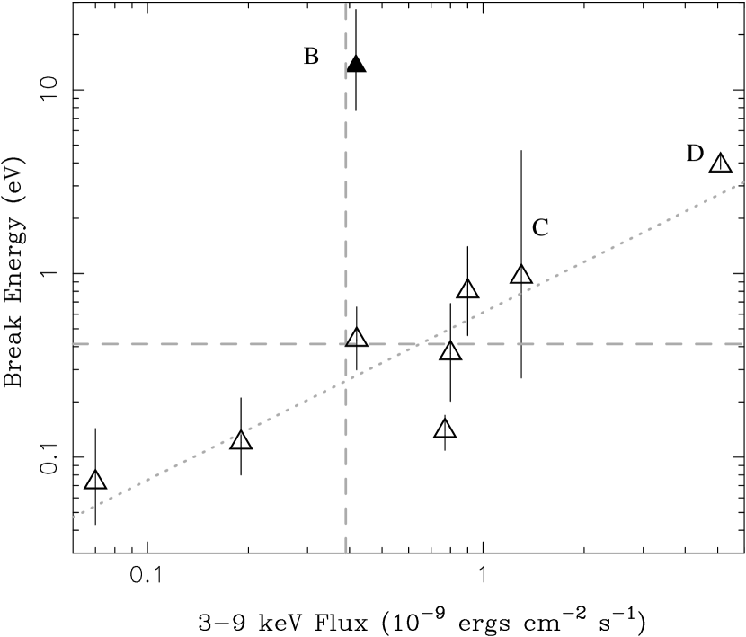
Figure 3.— Results of broken power-law fits to GX 339$-$4, showing the location of the break between the radio and soft X-ray power-law. Labels refer to Table 1, and are further described in the text. Here, and throughout the remaining figures, solid points will refer to observations A (not shown in the above ) and B, which have ‘optically thin’ radio spectra. Dashed lines show the approximate integrated X-ray flux and IR spectral break energy previously observed in GX 339$-$4 (Corbel & Fender 2002). The dotted line is $\propto{F_{\rm x}}^{0.91}$.

Phenomenologically speaking, the X-ray break is consistent with the expectations from reflection models (Magdziarz & Zdziarski 1995). However, as shown in Fig. 2, the identical broken power-law model described above provides a very good phenomenological description even for Cyg X-1 hard state data with an extreme break. Although not mutually exclusive with the presence of reflection, such data require at least two broad-band continuum components in the X-ray. For example, Fig. 2 could be consistent with synchrotron and synchrotron self-Compton from jet models (Markoff & Nowak 2004, Markoff, Nowak, & Wilms, in prep.), or a strong disk plus Comptonization component from corona models. These issues will be explored in greater detail in a forthcoming work (Wilms et al., in prep.).

2.2. Predicted Radio/X-ray Correlations

Given only two radio points and an X-ray spectrum that is well-fit by a singly broken power-law, it is not surprising that the doubly broken power-law models work as well. But how do the fitted locations of the radio-to-soft X-ray break compare to the ‘IR coincidence’ breaks, and how do the fitted break locations scale with observed flux? In Fig. 3 we show the fitted radio-to-X-ray break location as a function of 3–9 keV integrated flux. We also show in this figure the approximate integrated 3–9 keV flux and the IR break location for the 1997 observation discussed by Corbel & Fender (2002). For our GX 339$-$4 observations of comparable 3–9 keV flux, the doubly broken power-law models do indeed produce a break in the IR. Looking over the whole span of observed integrated X-ray fluxes, however, we see that the model fits presented here have predicted radio-to-X-ray breaks ranging all the way from the far IR to the blue end of the optical (and into the X-ray, if one also considers observation B [40108-01-04], which has an ‘optically thin’ radio spectrum).

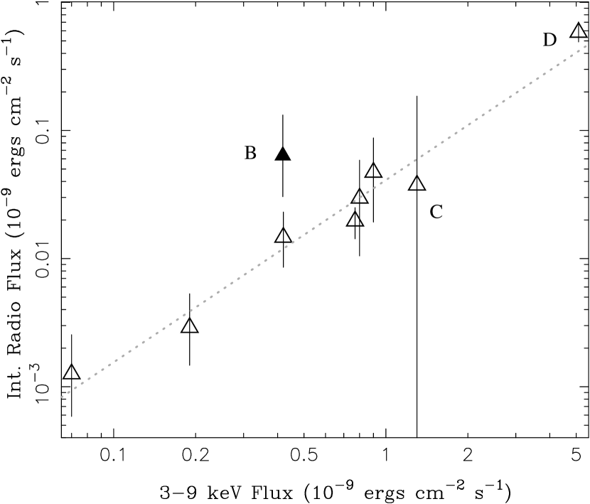
Figure 4.— The flux of the radio power-law, integrated from zero energy to the spectral break between the radio and soft X-ray, vs. the 3–9 keV (PCA) flux. Labels refer to Table 1 (Observation A not shown), and are further described in the text. The dotted line is $\propto{F_{\rm x}}^{1.4}$.

To assess the correlation of radio-to-X-ray break energy with integrated X-ray flux, we exclude observation B (40108-01-04), which has an optically thin radio spectrum, and perform a regression analysis on the remaining eight data points. We weight the data uniformly, which is equivalent to assuming that intrinsic variations in any correlation dominate over statistical errors. (In the results discussed below, the derived regression slopes and errors encompass the values obtained if one weights the data by their error bars.) We find that the radio-to-X-ray break energy, in eV, scales with the 3–9 keV integrated flux as $0.61{F_{\rm x}}^{0.91\pm 0.18}$. Does this agree with models wherein the observed soft X-ray spectrum is the optically thin synchrotron emission from a jet?

Using a scale invariance Ansatz to describe the jet physics (Heinz & Sunyaev 2003; Heinz 2004, see also Falcke & Biermann 1995 and Markoff et al. 2003), we can predict the scaling between the integrated X-ray synchrotron flux and the radio-to-X-ray break frequency where the jet becomes optically thin to synchrotron self-absorption. For simplicity, we make the assumption that, at the base of the jet, the fraction of particle pressure to magnetic pressure is independent of accretion rate/jet power.

Given the above assumptions, the optically thick radio flux follows (Heinz & Sunyaev 2003):

$${\cal F}_{\rm r}\propto B^{\frac{\scriptstyle[2p-(p+6)\alpha_{\rm r}+13]}{\scriptstyle[p+4]}}~{}~{},$$ (2)

where $\alpha_{\rm r}$ is the radio spectral index, $p$ is the power-law index of the electron spectrum (at energies below any synchrotron cooling regime), and $B$ is the magnetic field at the base of the jet. From Heinz (2004), using the same assumptions, the X-ray synchrotron flux integrated over a fixed energy band follows

$${F_{\rm x}}\propto B^{\scriptstyle[1+2p+3\alpha_{\rm x}]}~{}~{},$$ (3)

where $\alpha_{\rm x}$ is the X-ray spectral index. (We again are using the convention that $\alpha\equiv 1-\Gamma$.) Combining these expresions, we find

$${\cal F}_{\rm r}\propto{F_{\rm x}}^{\frac{\scriptstyle[2p-(p+6)\alpha_{\rm r}+13]}{\scriptstyle[p+4][1+2p+3\alpha_{\rm x}]}}~{}~{}.$$ (4)

If the X-ray band is unaffected by synchrotron cooling, the relation follows ${\cal F}_{\rm r}\propto{F_{\rm x}}^{0.69\rightarrow 0.81}$, for values of $2.6<p<2$, $-0.8<\alpha_{x}=(1-p)/2<-0.5$, and $0<\alpha_{\rm r}<0.2$. This scaling is consistent with previous observations, and is also consistent with prior descriptions of the jet model’s predictions (i.e., Corbel et al. 2003; Markoff et al. 2003).

The lower break frequency, $\nu_{\rm b}$, from an optically thick to optically thin spectrum is proportional to (Heinz & Sunyaev 2003)

$$\nu_{\rm b}\propto B^{\frac{\scriptstyle[6+p]}{\scriptstyle[4+p]}}~{}~{}.$$ (5)

We thus can write the dependence of $\nu_{\rm b}$ upon ${F_{\rm x}}$ as

$$\nu_{\rm b}\propto{F_{\rm x}}^{\frac{\scriptstyle[6+p]}{\scriptstyle[1+2p+3\alpha_{\rm x}][4+p]}}\propto{F_{\rm x}}^{\frac{\scriptstyle 2[p+6]}{\scriptstyle[p+4][p+5]}}~{}~{},$$ (6)

where for the latter relation we have used $\alpha_{\rm x}=(1-p)/2$ from standard synchrotron theory. Again taking $-0.8<\alpha_{\rm x}<-0.5$, we obtain $\nu_{\rm b}\propto F_{\rm x}^{0.34}$ to $\nu_{\rm b}\propto F_{\rm x}^{0.38}$. This prediction is flatter than the observed dependence of extrapolated break frequency upon X-ray flux.

Eq. (6) represents the scaling of the actual location of the break from an optically thick to optically thin spectrum (as appropriate for the ‘IR coincidence’ yielding the appropriate location of an observed break). Our observations instead yield the scaling of the inferred location of the break, which has an additional dependence upon the scalings of the spectral slopes, $\alpha_{\rm r}$ and ${\alpha_{\rm x}}$. Specifically, if one assumes that there is an underlying radio/X-ray correlation given by ${\cal F}_{\rm r}\propto{F_{\rm x}}^{\beta}$, yet allows evolution of the radio and X-ray spectral slopes, one can show that for the inferred break, $\nu_{\rm b}$,

$$\log\left(\frac{\nu_{\rm b}}{\nu_{\rm 0}}\right)~{}=~{}\left[\left(\alpha_{\rm r}-\alpha_{\rm x}\right)+\Delta\alpha_{\rm r}-\Delta\alpha_{\rm x}\right]^{-1}~{}\times~{}$$ (7)

$$\left[(1-\beta)\log\left(\frac{F_{\rm x}}{F_{0}}\right)+\log\left(\frac{\nu_{\rm r}}{\nu_{0}}\right)\Delta\alpha_{\rm r}-\log\left(\frac{\nu_{\rm x}}{\nu_{0}}\right)\Delta\alpha_{\rm x}\right]~{},$$ (8)

where $\nu_{0}$ is the break energy measured at an X-ray flux of $F_{0}$, $\nu_{\rm r}$, and $\nu_{\rm x}$ are the frequencies at which the radio and X-ray fluxes, respectively, are measured, and $\Delta\alpha_{\rm r}$ and $\Delta\alpha_{\rm x}$ are the changes in radio and X-ray spectral indices as the X-ray flux changes to $F_{\rm x}$. (Note that small correction factors for the dependence of integrated X-ray flux upon $\alpha_{\rm x}$, as opposed to solely power law normalization, have been omitted.)

In the absence of evolution of the spectral indices, one expects the break frequency to scale with X-ray flux with a power of $(1-\beta)/(\alpha_{\rm r}-\alpha_{\rm x})\approx 0.35$, as described above. However, as noted elsewhere (Wilms et al. 1999; Nowak et al. 2002), many of the observations of GX 339$-$4 show a softening/hardening with increasing/decreasing X-ray flux. (For sources with optically thick radio spectra, notable exceptions to this trend are Obs IDs 40108-02-03 and 70109-01-02. A detailed discussion of flux/hardness trends can be found in Nowak et al. 2002.) Comparing Obs ID 40108-02-02 to 20181-01-01, $\Delta\alpha_{\rm x}\approx 0.06$ for $\log(F_{\rm x}/F_{0})\approx 0.7$. Combining this with $\alpha_{\rm r}+\alpha_{\rm x}\approx 0.8$ and $\log(\nu_{\rm x}/\nu_{0})\approx 4.9$ means that the break energy should scale with with X-ray flux with a power of $(1-\beta+0.5)/0.8\approx 1$. This is in much closer agreement with the observed trends.

Contrary to $\alpha_{\rm x}$, there are no obvious trends for a dependence of $\alpha_{\rm r}$ upon X-ray flux. (This will be explored in a future work, with a larger set of observations from 2002 and 2004 outbursts of GX 339$-$4; Corbel et al., in prep.) The mean value for all the optically thick radio data is $\langle\alpha_{\rm r}\rangle=0.16$, with a scatter of $\pm 0.05$. Combining this with $\log(\nu_{\rm r}/\nu_{0})\approx-3.5$, and the fact that from the faintest to brightest observation is a factor of $10^{1.9}$, we expect the variations in radio slope to account for correlation slope variations of up to $\pm 0.1$.

We thus find that the observed correlation of inferred break energy is inconsistent with the expectations from the very simplest X-ray synchrotron jet model (i.e., the jet spectra scaling with input power, and no evolution of the radio or X-ray slopes). The observed trends can be recovered, however, if the differences from the simplest expectations are primarily driven by evolution of the X-ray spectral slope, $\alpha_{\rm x}$, with X-ray flux, with possible lesser contributions from variations of the radio spectral slope, $\alpha_{\rm r}$. We shall discuss this point further in §5.

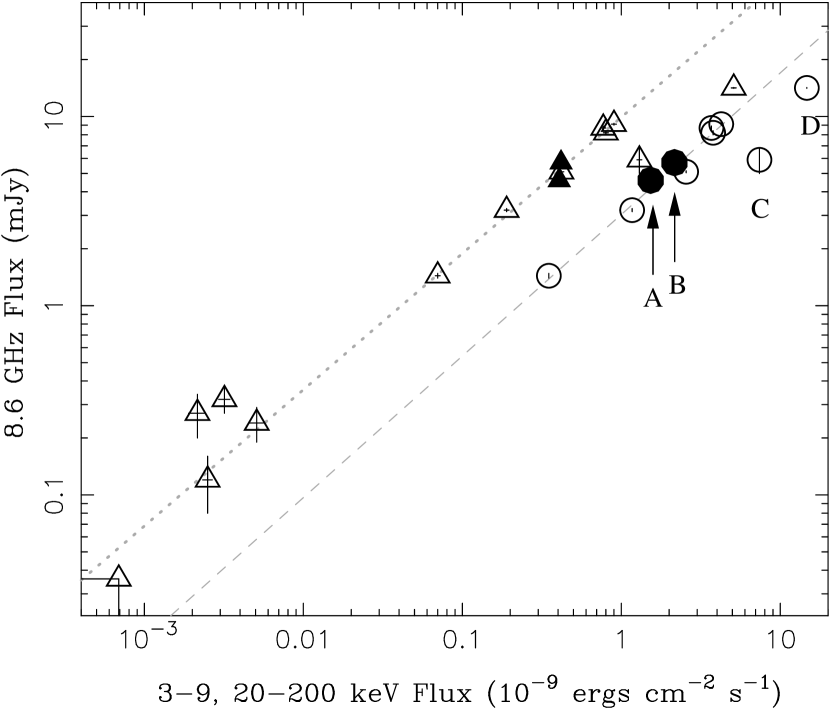
Figure 5.— 3–9 keV (triangles) and 20–200 keV (circles) X-ray flux (units of $10^{-9}~{}{\rm ergs~{}cm~{}s^{-1}}$) from pointed RXTE observations of GX 339$-$4 vs. 8.6 GHz radio flux (mJy). Labels refer to Table 1, and are further described in the text. Lines show power-laws of the form ${F_{\rm x}}^{b}$, with $b=0.72$ (dotted line) and $b=0.75$ (dashed line).

A further interesting correlation is seen when one looks at the dependence of radio flux, integrated between zero energy and the break frequency, upon the integrated X-ray flux, as we show in Fig. 4. Considering both in units of $10^{-9}~{}{\rm erg~{}cm^{-2}~{}s^{-1}}$, and again weighting the data uniformly, we find ${F_{\rm r}}=0.04{F_{\rm x}}^{1.42\pm 0.10}$. This implies that, even ignoring the energy of the particles and fields in the jet, the ‘jet radiation’ up to the inferred break is 3–10% of the integrated 3–9 keV X-ray flux, and is 0.5–5% of the 3–200 keV flux.

Again, we can compare this result to expectations from the simplest jet models. Utilizing our previous estimates, we find for the product of ${\cal F}_{\rm r}\nu_{\rm b}$:

$${\cal F}_{\rm r}\nu_{\rm b}\propto F_{\rm x}^{\frac{\scriptstyle[19+3p-\alpha_{\rm r}(p+6)]}{\scriptstyle[p+4][1+2p+3\alpha_{\rm x}]}}$$ (9)

Again using the range of $-0.8<\alpha_{\rm x}<-0.5$ and $0<\alpha_{\rm r}<-0.2$, this product should follow ${\cal F}_{\rm r}\nu_{\rm b}\propto{F_{\rm x}}^{1\rightarrow 1.19}$. As before, for the inferred value we might expect to increase the scaling exponent by $0.5\pm 0.1$, if we allow for an evolution of $\alpha_{\rm r}$ and $\alpha_{\rm x}$ with X-ray flux.

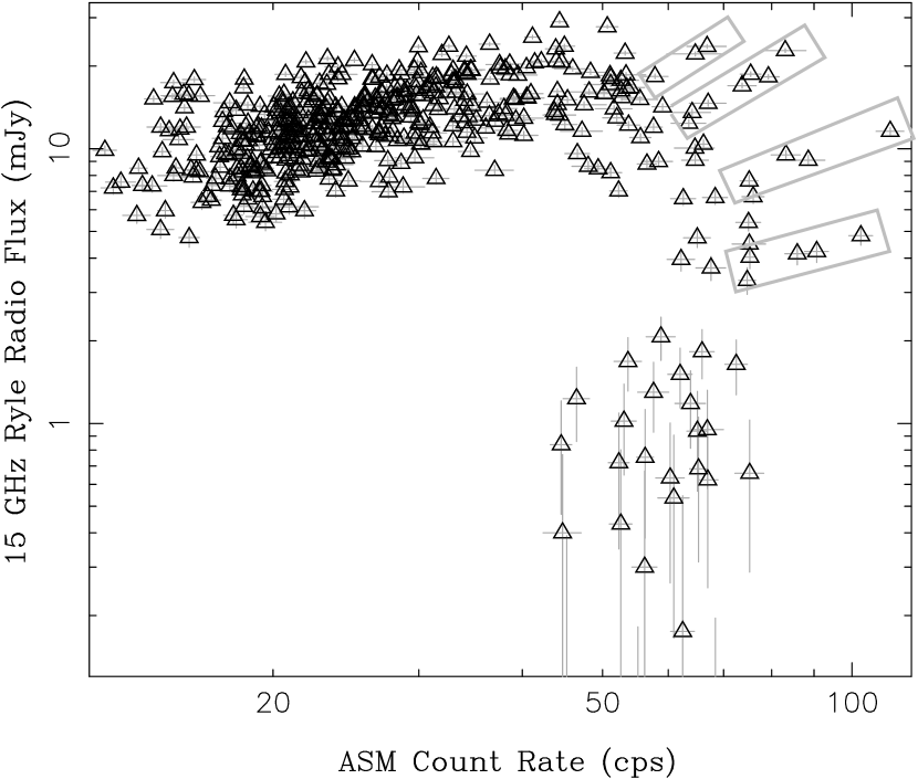
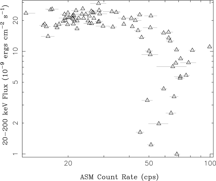
Figure 6.— Left: 15 GHz Ryle radio flux (mJy) vs. Cyg X-1 daily mean ASM count rate (see text). Grey boxes highlight data associated with failed state transitions, and the beginning of a transition to a prolonged soft state. Right: 20–200 keV flux (units of $10^{-9}~{}{\rm ergs~{}cm~{}s^{-1}}$) from pointed RXTE observations. vs. Cyg X-1 daily mean ASM count rate (see text).

3. Radio/X-ray Correlations in GX 339$-$4

One of the interesting aspects of the radio/X-ray flux correlation in GX 339$-$4 as identified by Corbel et al. (2003) is that it appeared to be consistent in both slope and amplitude between the 1997 and 1999 low/hard states, despite the intervening radio quiet, soft state outburst (see Fig. 5). The high luminosity observations C and D [70109-01-02 and 40031-03-01], however, were not part of the original correlation presented by Corbel et al. (2003). These two observations occurred in 2002, 14 days apart, in a bright hard state as GX 339$-$4 was rising into an even brighter soft state.

In Fig. 5 we plot the 8.6 GHz radio flux density vs. the 3–9 and 20–200 keV X-ray fluxes. As in Corbel et al. (2003), we have performed a regression fit for all the 1997 and 1999 observations for which we could determine both a 3–9 keV (PCA) and 20–200 keV (HEXTE) flux. (However, we also plot the 1999 low flux observations from Corbel et al. 2003 that have only PCA data.) For the soft X-rays we find ${\cal F}_{\rm r}=9.9{F_{\rm x}}^{0.73\pm 0.02}$, and for the hard X-rays we find ${\cal F}_{\rm r}=3.0{F_{\rm x}}^{0.75\pm 0.02}$. The slight differences between these correlation slopes and those presented by Corbel et al. (2003) are due to our use of better calibrated RXTE response matrices (especially for the PCA). As discussed by Corbel et al. (2003), the correlations apply equally well to the 1997 and the 1999 data, including the low flux 1999 data that were not formally part of the regression fit. The slopes between the soft and hard X-rays are also reasonably consistent with one another (Corbel et al. 2003).

The 2002 data, although only consisting of two points, deviate from these previously viewed trends. For these data, the radio flux vs. the 3–9 keV flux correlation appears to have the expected slope, but more than a factor of two times lower amplitude. The radio/hard X-ray correlation, however, appears to be less reduced in amplitude, but has a steeper slope, with ${\cal F}_{\rm r}\propto{F_{\rm x}}^{1.3}$. There is one major uncertainty in these results: the radio data associated with observations C and D were not strictly simultaneous with the X-ray data. We note, however, that the radio data, which falls below the previously observed trends, was taken after the X-ray data while the source was rising in flux on several day time scales.

It is also possible that observations C and D, rather than being on a lower radio amplitude parallel track, are instead indicating a turnover in the correlation occuring at high X-ray flux. Such a turnover has been observed for the correlation seen in Cyg X-1 (Gallo et al. 2003, and Fig. 6). If this latter hypothesis is correct, then given the observed 14.2 mJy flux for the highest flux observation, D, the deficit is a factor of 2.3 for the 3–9 keV correlation (which predicts 32.4 mJy), but only a factor of 1.6 for the 20–200 keV flux correlation (which predicts 22.7 mJy). Extrapolating the observed 2.4 GHz radio flux for observation C to 8.64 GHz yields $5.9\pm 0.9$ mJy. This is a factor of $2^{+0.4}_{-0.2}$ below the value predicted by the radio/3–9 keV flux correlation, and a factor of $2.2^{+0.4}_{-0.3}$ below the value predicted by the radio/20–200 keV flux correlation.

A further interesting fact to note also comes from the radio/hard X-ray correlation. Observations A and B (40108-01-03 and 40108-01-04) were the first observations taken after the 1999 return to the radio-loud hard state, and both have optically thin (i.e., $\alpha_{\rm r}<0$) radio spectra. Although they have nearly identical 3–9 keV integrated fluxes, they have different radio fluxes and they straddle the radio/soft X-ray flux correlation shown in Fig. 5. However, these points actually lie along the radio/hard X-ray flux correlation, as they have significantly different 20–200 keV fluxes. This might argue that the radio/hard X-ray flux is the more fundamental relationship.

4. Radio/X-ray Correlations in Cyg X-1

The radio/X-ray correlations in GX 339$-$4 present us with two, not necessarily mutually exclusive, possibilities. Either the radio/X-ray correlation is more fundamentally tied to the hard X-rays, and/or different instances of the hard state can present the correlation with different amplitudes. To further explore these possibilities, we turn to radio/X-ray observations of Cyg X-1 (Pottschmidt et al. 2003; Gallo et al. 2003). As described in Pottschmidt et al. (2003), the radio data are 15 GHz observations performed at the Ryle Telescope, Cambridge (UK). These are single channel observations, so a radio spectral slope cannot be determined. Most of these observations have occurred simultaneously with pointed RXTE observations (Pottschmidt et al. 2003), and nearly all have very good contemporaneous coverage by the RXTE All Sky Monitor (ASM). The ASM provides coverage in the 1.5–12 keV energy band (Remillard & Levine 1997), and therefore allows us to assess the radio/soft X-ray correlation in Cyg X-1.

In Fig. 6 we plot the daily average ASM count rate vs. the daily average 15 GHz flux. Here we only include days for which there are at least 25 ASM data points (representing 70 second dwells) with a reduced $\chi^{2}<1.5$ for the ASM solution (see Remillard & Levine 1997). Ranging from approximately 10–50 cps in the ASM  there is a clear log-linear correlation between the radio flux and the ASM count rate. As for GX 339$-$4, the radio flux rises more slowly than the ASM count rate (${\cal F}_{\rm r}$ scales approximately as the 0.8 power of the ASM count rate). Cyg X-1, however, shows much more scatter in the amplitude of the correlation than does GX 339$-$4. This scatter is not dominated by variations related to the orbital phase of the binary system (cf., Brocksopp et al. 1999).

As noted by Gallo et al. (2003), there is a sharp roll-over for higher ASM count rates. However, one can clearly discern on the shoulder of this roll-over (i.e., the upper right corner of Fig. 6) four ‘spokes’, consisting of 2–5 data points each. In these spokes, the radio/X-ray correlation appears to hold to high count rates. We have confirmed that each of these times are associated with ‘failed transitions’ to the soft state, as described by Pottschmidt et al. (2003), except for the lowest amplitude of these spokes, which occurs immediately preceding a prolonged soft state outburst. In many ways these failed state transitions and the early stage of a soft state outburst for Cyg X-1 are reminiscent of the data presented here for the 2002 GX 339$-$4 hard state. As for those latter GX 339$-$4 data, the Cyg X-1 spectra remain hard, although not as hard as low-luminosity hard states, to very high flux levels.

In Fig. 6 we also plot the daily average ASM count rate vs. the 20–200 keV flux from our pointed RXTE observations taken during the same 24 hour period (Pottschmidt et al. 2003). Here, however, we only require 3 ASM data points per average, for a resulting 85 observations. We see that hard X-ray/ASM correlation traces a similar pattern to the radio/ASM correlation. Indeed, when we plot the hard X-ray flux vs. the daily average radio flux (representing 129 separate hard X-ray pointed observations), we obtain a log-linear relationship, as shown in Fig. 7 (see also Gleissner et al. 2004). (Two high radio flux, but low X-ray flux, data points are seen in the upper left of this figure; these represent intra-day hard X-ray variations.) Returning to the question that we posed in §4 of whether we were seeing evidence for parallel tracks in the radio/X-ray correlation, or whether we were seeing the correlation being more fundamental to the hard X-ray band, in Cyg X-1 the answer seems to be that both effects are discernible, but fundamentally the radio flux density does appear to be tied to the hard X-ray emission.

5. Summary

In this work we have considered ten simultaneous or near simultaneous RXTE/radio observations of GX 339$-$4, and over one hundred RXTE/radio observations of Cyg X-1. We have fit the former spectra with a very simple, but remarkably successful, phenomenological model consisting of a doubly broken power-law with an exponential roll-over plus a gaussian line. For GX 339$-$4, the break between the radio and soft X-ray power-laws occurs in the IR to optical range, in agreement with the prior work of Motch et al. (1985) and Corbel & Fender (2002) (i.e., the ‘IR coincidence’). In contrast to these prior works, we have fit the X-ray data in ‘detector space’ and provided a quantitative assessment of the extrapolated break location.

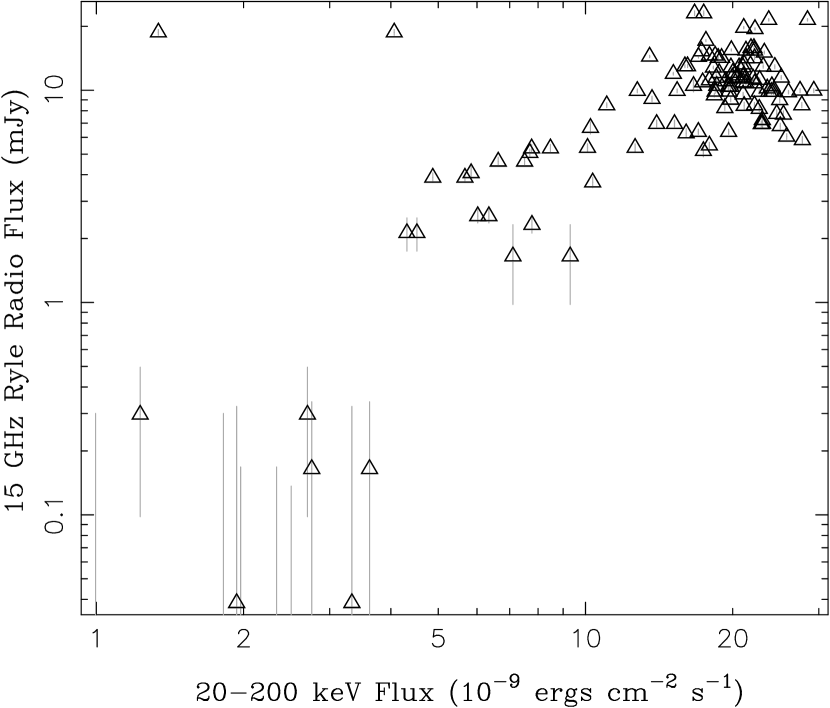
Figure 7.— 20–200 keV flux (units of $10^{-9}~{}{\rm ergs~{}cm~{}s^{-1}}$) vs. the daily average 15 GHz Ryle radio flux (mJy) for pointed observations of Cyg X-1.

Is the ‘IR coincidence’ just a coincidence? The spectral fits to the GX 339$-$4 data suggest that the answer is ‘possibly not’. All of the data with optically thick radio spectra are extremely well-fit by doubly broken power-laws, with the break being in the IR regime. Although the scaling of this break frequency with X-ray flux does not agree with the predictions of the simplest X-ray synchrotron jet models, if one allows for softening of the X-ray spectrum with increasing X-ray flux, then the jet model predictions agree with the observed correlations. There are several possibilities why such a softening could occur. In terms of the jet model, for example, there could be cooling of the electron spectrum leading to a steepening in the X-rays. A second possibility is that the soft X-rays are being contaminated by excess emission from a disk component that becomes more prominent with increasing flux. What is clear is that in order for jet models to explain both the scaling of ${\cal F}_{\rm r}\propto{F_{\rm r}}^{0.72}$ and $\nu_{b}\propto{F_{\rm r}}^{0.92}$, they must be more sophisticated than the very simplest considerations. Fits to some of these data sets with such models, which include disk emission, synchrotron self-Compton emission, etc., are currently being considered in detail, and will be discussed in a future work (Markoff, Nowak, & Wilms, in prep.). The results presented here, however, are consistent with the notion that at least some fraction of the observed soft X-rays may be attributable to emission from the jet, as opposed to disk or corona.

On the other hand, other facts suggest that the answer to the question of the ‘IR coincidence’ being just that is ‘maybe’. We have tentative evidence in GX 339$-$4, and firmer evidence in the Cyg X-1 failed state transitions and soft state transition, that the correlation between radio flux and integrated X-ray flux can take on different amplitudes during different hard state episodes. There is also evidence in Cyg X-1 that the radio/X-ray correlation is more fundamental to the hard X-ray band. In jet models, this band, which essentially encompasses the third, highest energy, power-law component in our model fits (and also encompasses the exponential cutoff), is possibly attributable to the synchrotron self-Compton (SSC) emission from the base of the jet (see, e.g., Markoff et al. 2003; Markoff & Nowak 2004). It is therefore quite reasonable to expect a strong coupling between the radio and hard X-ray flux; however, these models are more complex than simple pure synchrotron models, and are only now beginning to be explored quantitatively (Markoff et al. 2003; Markoff & Nowak 2004). It is also worth noting that such radio/X-ray couplings can be expected in Compton corona models (e.g., Meier 2001; Merloni & Fabian 2002).

More problematic for pure jet models are GX 339$-$4 observations A and B (40108-01-03, 40108-01-04), both of which occurred very shortly after the 1999 return to the hard state. They have ‘typical’ hard state properties in terms of spectra and variability (Nowak et al. 2002), but have optically thin radio spectra that do not neatly extrapolate into the observed soft X-ray spectra. They satisfy the radio flux density/integrated X-ray flux correlation; however, they agree better with the radio/hard X-ray flux correlation, for which these two observations are cleanly differentiated from one another (Fig. 5). It is possible that they represent an early, transient phase of the jet as it forms. It then remains a theoretical question for the jet model whether it can describe a scenario where the basic radio/X-ray flux correlation and ‘typical’ steady-state X-ray spectra hold, while the radio has not yet settled into a steady ‘optically thick’ state.

The results presented here suggest, at the very least, some obvious observational strategies to arrive at a more definitive answer to the question that we have posed. Given the break energy correlations, it would be extremely useful to have not only a radio amplitude for each X-ray observation, but also a radio slope. Furthermore, the inferred break for the brightest observation, D (40031-03-01), occurs in the blue end of the optical. Thus, ideally multi-wavelength observations would consist of radio, broad band X-ray, and IR through optical coverage (see, for example, Hynes et al. 2003; Malzac et al. 2004, which suggest the possibility of jet synchrotron radiation extending into the optical regime for the hard state of XTE J1118+48). This is an admittedly difficult task, but BHC are demonstrating via spectral correlations that all these energy regimes are fundamentally related to activity near the central engine, i.e., the black hole, of the system.

Finally, it is important to obtain multi-wavelength observations of multiple episodes of each of the spectral states. For example, if there are indeed ‘parallel tracks’ in the radio/X-ray correlations, it would be interesting to determine whether the amplitude of the radio/X-ray correlation is related to the flux at which the outbursting source transits from the low/hard to high/soft state. We note that the low amplitude radio/X-ray correlation of the 2002 GX 339$-$4 outburst was associated with a very high flux level for the hard-to-soft state transition. The low amplitude ‘spokes’ in the Cyg X-1 radio/X-ray correlation might be similar in that they are associated with failed state transitions. If such observations can be made with more quantitative detail, we will have vital clues to determining the relative contributions of coronae and jets, and the coupling between these two components, for black hole binary systems.

Table 1GX 339$-$4 Observed Fluxes (1$\sigma$ confidence).

Obs ID		y.m.d	0.84 GHz	1.38 GHz	2.40 GHz	4.80 GHz	8.64 GHz	3–9 keV	9–20 keV	20–100 keV	100–200 keV
			(mJy)					(${\rm 10^{-9}~{}ergs~{}cm^{-2}~{}s^{-1}}$)
20181-01-01		1997.02.03	$7.0^{+0.6}_{-0.6}$	$\cdots$	$\cdots$	$\cdots$	$9.1^{+0.1}_{-0.1}$	0.90	0.92	2.98	1.27
20181-01-02		1997.02.10	$5.5^{+0.7}_{-0.7}$	$\cdots$	$\cdots$	$\cdots$	$8.2^{+0.2}_{-0.2}$	0.80	0.82	2.67	1.11
20181-01-03		1997.02.17	$5.6^{+0.7}_{-0.7}$	$5.4^{+0.2}_{-0.2}$	$6.0^{+0.2}_{-0.2}$	$\cdots$	$8.7^{+0.2}_{-0.2}$	0.77	0.78	2.63	1.06
40108-01-03	A	1999.02.12	$\cdots$	$\cdots$	$\cdots$	$6.34^{+0.08}_{-0.08}$	$4.60^{+0.08}_{-0.08}$	0.41	0.39	1.18	0.48
40108-01-04	B	1999.03.03	$\cdots$	$\cdots$	$\cdots$	$6.07^{+0.06}_{-0.06}$	$5.74^{+0.06}_{-0.06}$	0.42	0.42	1.51	0.66
40108-02-01		1999.04.02	$\cdots$	$\cdots$	$\cdots$	$4.75^{+0.06}_{-0.06}$	$5.10^{+0.06}_{-0.06}$	0.42	0.44	1.60	0.97
40108-02-02		1999.04.22	$\cdots$	$\cdots$	$\cdots$	$2.92^{+0.06}_{-0.06}$	$3.20^{+0.06}_{-0.06}$	0.19	0.21	0.74	0.43
40108-02-03		1999.05.14	$\cdots$	$\cdots$	$\cdots$	$1.25^{+0.06}_{-0.06}$	$1.44^{+0.06}_{-0.06}$	0.07	0.07	0.21	0.14
70109-01-02	C	2002.04.03	$\cdots$	$4.83^{+0.20}_{-0.20}$	$5.13^{+0.11}_{-0.11}$	$\cdots$	$\cdots$	1.30	1.47	5.34	2.09
40031-03-01	D	2002.04.18	$\cdots$	$\cdots$	$\cdots$	$13.04^{+0.06}_{-0.06}$	$14.16^{+0.07}_{-0.07}$	5.10	4.97	12.3	2.42

Note. — X-ray flux errors are taken to be 3.5%, the average of the fitted normalization difference between PCA and HEXTE, since this exceeds the statistical uncertainties.

Table 2GX 339$-$4 Spectral Fits (90% Confidence Level errors).

Obs ID		${\rm E_{cut}}$	${\rm E_{fold}}$	$\alpha_{\rm r}$	${\rm E_{b-r}}$	$\Gamma_{\rm soft}$	${\rm E_{b-x}}$	$\Gamma_{\rm hard}$	${\rm A_{line}}$	$\sigma_{\rm line}$	Con.	$\chi^{2}$/DoF
		(keV)	(keV)		(eV)		(keV)		($10^{-3}$ )	(keV)
20181-01-01		$37^{+7}_{-6}$	$155^{+22}_{-19}$	$0.11^{+0.08}_{-0.07}$	$0.80^{+1.22}_{-0.48}$	$1.69^{+0.01}_{-0.01}$	$11.3^{+0.6}_{-0.5}$	$1.49^{+0.03}_{-0.02}$	$2.1^{+0.2}_{-0.3}$	$0.6^{+0.1}_{-0.1}$	$0.97^{+0.01}_{-0.02}$	110/108
20181-01-02		$42^{+5}_{-5}$	$140^{+16}_{-14}$	$0.17^{+0.10}_{-0.09}$	$0.37^{+0.66}_{-0.23}$	$1.68^{+0.01}_{-0.00}$	$11.0^{+0.6}_{-0.5}$	$1.48^{+0.02}_{-0.02}$	$1.8^{+0.3}_{-0.2}$	$0.7^{+0.1}_{-0.2}$	$0.95^{+0.01}_{-0.01}$	162/114
20181-01-03		$53^{+14}_{-8}$	$133^{+33}_{-31}$	$0.26^{+0.04}_{-0.04}$	$1.39^{+0.61}_{-0.40}$	$1.68^{+0.01}_{-0.00}$	$10.7^{+0.6}_{-0.7}$	$1.51^{+0.02}_{-0.02}$	$1.7^{+0.2}_{-0.2}$	$0.6^{+0.1}_{-0.1}$	$0.98^{+0.02}_{-0.02}$	90/90
40108-01-03	A	$44^{+9}_{-11}$	$165^{+58}_{-41}$	$\cdots$	$\cdots$	$1.80^{+0.01}_{-0.01}$	$10.2^{+1.0}_{-0.5}$	$1.59^{+0.02}_{-0.03}$	$1.2^{+0.1}_{-0.2}$	$0.7^{+0.1}_{-0.1}$	$1.03^{+0.01}_{-0.01}$	64/77
40108-01-04	B	$69^{+14}_{-13}$	$138^{+59}_{-48}$	$-0.09^{+0.04}_{-0.05}$	$13.5^{+37.}_{-8.0}$	$1.69^{+0.01}_{-0.01}$	$10.6^{+0.6}_{-0.7}$	$1.53^{+0.01}_{-0.02}$	$0.9^{+0.1}_{-0.1}$	$0.6^{+0.1}_{-0.2}$	$1.03^{+0.02}_{-0.02}$	106/103
40108-02-01		$32^{+21}_{-8}$	$345^{+133}_{-79}$	$0.12^{+0.06}_{-0.05}$	$0.44^{+0.43}_{-0.20}$	$1.67^{+0.01}_{-0.01}$	$10.5^{+0.6}_{-0.6}$	$1.45^{+0.03}_{-0.02}$	$0.7^{+0.2}_{-0.1}$	$0.5^{+0.2}_{-0.2}$	$0.97^{+0.02}_{-0.02}$	115/93
40108-02-02		$44^{+33}_{-18}$	$304^{+322}_{-142}$	$0.16^{+0.07}_{-0.08}$	$0.12^{+0.18}_{-0.06}$	$1.63^{+0.01}_{-0.01}$	$10.7^{+1.2}_{-1.4}$	$1.47^{+0.03}_{-0.05}$	$0.4^{+0.1}_{-0.1}$	$0.5^{+0.1}_{-0.2}$	$0.95^{+0.03}_{-0.03}$	83/67
40108-02-03		$\cdots$	$\cdots$	$0.24^{+0.12}_{-0.12}$	$0.07^{+0.16}_{-0.04}$	$1.68^{+0.01}_{-0.02}$	$9.0^{+3.}_{-0.0}$	$1.62^{+0.03}_{-0.05}$	$0.1^{+0.1}_{-0.0}$	$0.6^{+0.2}_{-0.3}$	$0.95^{+0.07}_{-0.08}$	26/44
70109-01-02	C	$34^{+2}_{-2}$	$112^{+6}_{-5}$	$0.11^{+0.14}_{-0.11}$	$0.95^{+14.3}_{-0.81}$	$1.61^{+0.01}_{-0.01}$	$10.3^{+0.4}_{-0.4}$	$1.37^{+0.01}_{-0.02}$	$2.2^{+0.3}_{-0.4}$	$0.4^{+0.1}_{-0.1}$	$0.99^{+0.01}_{-0.01}$	180/148
40031-03-01	D	$26^{+1}_{-2}$	$69^{+2}_{-3}$	$0.14^{+0.02}_{-0.01}$	$3.88^{+0.69}_{-0.41}$	$1.73^{+0.01}_{-0.01}$	$11.1^{+0.5}_{-0.5}$	$1.53^{+0.02}_{-0.03}$	$17.7^{+2.0}_{-1.8}$	$0.8^{+0.1}_{-0.1}$	$0.99^{+0.02}_{-0.01}$	143/130

Note. — 20181 data are from the 1997 hard state (Wilms et al. 1999; Nowak, Wilms, & Dove 2002), 40108 data are from the 1999 hard state (post-1998 soft state; Nowak, Wilms, & Dove 2002), 70109 and 40031 data are from the 2002 very luminous hard state (post a 3 year duration quiescent state; Homan et al. 2004). Parameters in italics were held fixed at that value for the fits. Note that the radio spectral index, $\alpha_{\rm r}$, is defined to be positive for ‘optically thick’ spectra, and is related to the usual X-ray astronomy definition of the photon index by $\alpha_{\rm r}=1-\Gamma_{\rm r}$.

References

- Arnaud (1996) Arnaud, K. A. 1996, in Astronomical Data Analysis Software and Systems V, ed. J. H. Jacoby & J. Barnes, Astron. Soc. Pacific, Conf. Ser. No. 101 (San Francisco: Astron. Soc. Pacific), 17
- Braes & Miley (1971) Braes, L. L. E. & Miley, G. K. 1971, Nature, 232, 246
- Brocksopp et al. (1999) Brocksopp, C., Fender, R. P., Larionov, V., Lyuty, V. M., Tarasov, A. E., Pooley, G. G., Paciesas, W. S., & Roche, P. 1999, MNRAS, 309, 1063
- Corbel & Fender (2002) Corbel, S. & Fender, R. P. 2002, ApJ, 573, L35
- Corbel et al. (2000) Corbel, S., Fender, R. P., Tzioumis, A. K., Nowak, M., McIntyre, V., Durouchoux, P., & Sood, R. 2000, A&A, 359, 251
- Corbel et al. (2003) Corbel, S., Nowak, M. A., Fender, R. P., Tzioumis, A. K., & Markoff, S. 2003, A&A, 400, 1007
- Falcke & Biermann (1995) Falcke, H. & Biermann, P. L. 1995, A&A, 293, 665
- Falcke et al. (2004) Falcke, H., Körding, E., & Markoff, S. 2004, A&A, 414, 895
- Fender et al. (1999) Fender, R., Corbel, S., Tzioumis, T., McIntyre, V., Campbell-Wilson, D., Nowak, M., Sood, R., Hunstead, R., Harmon, A., Durouchoux, P., & Heindl, W. 1999, ApJ, 519, L165
- Fender et al. (2003) Fender, R. P., Gallo, E., & Jonker, P. G. 2003, MNRAS, 343, L99
- Gallo et al. (2003) Gallo, E., Fender, R. P., & Pooley, G. G. 2003, MNRAS, 344, 60
- Gleissner et al. (2004) Gleissner, T., Wilms, J., Pooley, G. G., Nowak, M. A., Pottschmidt, K., Markoff, S., Heinz, S., Klein-Wolt, M., Fender, R. P., & Staubert, R. 2004, A&A, 425, 1061
- Hannikainen et al. (1998) Hannikainen, D. C., Hunstead, R. W., Campbell-Wilson, D., & Sood, R. K. 1998, A&A, 337, 460
- Heinz (2004) Heinz, S. 2004, MNRAS, 355, 835
- Heinz & Sunyaev (2003) Heinz, S. & Sunyaev, R. A. 2003, MNRAS, 343, L59
- Homan et al. (2004) Homan, J., Buxton, M., Markoff, S., Bailyn, C., Nespoli, E., & Belloni, T. 2004, ApJ, submitted
- Houck & Denicola (2000) Houck, J. C. & Denicola, L. A. 2000, in ASP Conf. Ser. 216: Astronomical Data Analysis Software and Systems IX, Vol. 9, 591
- Hynes et al. (2003) Hynes, R. I., Haswell, C. A., Cui, W., Shrader, C. R., O’Brien, K., Chaty, S., Skillman, D. R., Patterson, J., & Horne, K. 2003, MNRAS, 345, 292
- Kong et al. (2000) Kong, A. K. H., Kuulkers, E., Charles, P. A., & Homer, L. 2000, MNRAS, 312, L49
- Magdziarz & Zdziarski (1995) Magdziarz, P. & Zdziarski, A. A. 1995, MNRAS, 273, 837
- Malzac et al. (2004) Malzac, J., Merloni, A., & Fabian, A. C. 2004, MNRAS, 351, 253
- Markoff et al. (2001) Markoff, S., Falcke, H., & Fender, R. 2001, ApJ, 372, L25
- Markoff & Nowak (2004) Markoff, S. & Nowak, M. 2004, ApJ, 609, 972
- Markoff et al. (2003) Markoff, S., Nowak, M., Corbel, S., Fender, R., & Falcke, H. 2003, A&A, 397, 645
- Meier (2001) Meier, D. L. 2001, ApJ, 548, L9
- Merloni & Fabian (2002) Merloni, A. & Fabian, A. C. 2002, MNRAS, 332, 165
- Merloni et al. (2003) Merloni, A., Heinz, S., & di Matteo, T. 2003, MNRAS, 345, 1057
- Motch et al. (1985) Motch, C., Ilovaisky, S. A., Chevalier, C., & Angebault, P. 1985, Space Sci. Rev., 40, 219
- Noble (2005) Noble, M. 2005, in Proceedings of ADASS XIV, in press (astro–ph/0412003)
- Nowak et al. (2002) Nowak, M. A., Wilms, J., & Dove, J. B. 2002, MNRAS, 332, 856
- Pooley et al. (1998) Pooley, G. G., Fender, R. P., & Brocksopp, C. 1998, MNRAS, 302, L1
- Pottschmidt et al. (2003) Pottschmidt, K., Wilms, J., Chernyakova, M., Nowak, M. A., Rodriguez, J., Zdziarski, A. A., Beckmann, V., Kretschmar, P., Gleissner, T., Pooley, G. G., Martínez-Núñez, S., Courvoisier, T. J.-L., Schönfelder, V., & Staubert, R. 2003, A&A, 411, L383
- Pottschmidt et al. (2003) Pottschmidt, K., Wilms, J., Nowak, M. A., Pooley, G. G., Gleissner, T., Heindl, W. A., Smith, D. M., Remillard, R., & Staubert, R. 2003, A&A, 407, 1039
- Remillard & Levine (1997) Remillard, R. A. & Levine, A. M. 1997, in All-Sky X-Ray Observations in the Next Decade, ed. N. Matsuoka & N. Kawai (Tokyo: Riken), 29
- Sood & Campell-Wilson (1994) Sood, R. & Campell-Wilson, D. 1994, IAU Circ. 6006
- Stirling et al. (2001) Stirling, A. M., Spencer, R. E., de la Force, C. J., Garrett, M. A., Fender, R. P., & Ogley, R. N. 2001, MNRAS, 327, 1273
- Sunyaev & Trümper (1979) Sunyaev, R. A. & Trümper, J. 1979, Nature, 279, 506
- Wardziński et al. (2002) Wardziński, G., Zdziarski, A. A., Gierliński, M., Grove, J. E., Jahoda, K., & Johnson, W. N. 2002, MNRAS, 337, 829
- Wilms et al. (1999) Wilms, J., Nowak, M. A., Dove, J. B., Fender, R. P., & di Matteo, T. 1999, ApJ, 522, 460