The Vela Pulsar in the Ultraviolet

Abstract

We describe time-tagged observations of the Vela pulsar (PSR B0833$-$45) with the HST STIS MAMA-UV detectors. Using an optimal extraction technique, we obtain a NUV light curve and crude FUV phase-resolved spectra. The pulse is dominated by complex non-thermal emission at all phases. We obtain approximate spectral indices for the brightest pulse components, relate these to pulsations observed in other wavebands, and constrain the thermal surface emission from the neutron star. An upper limit on the Rayleigh-Jeans component at UV pulse minimum suggests a rather low mean surface temperature $T_{\rm eff}^{\infty}<4.6\times 10^{5}(d_{300}/R_{14.2})^{2}$K. If confirmed by improved phase-resolved spectroscopy, this observation has significant impact on our understanding of neutron star interiors.

1 Introduction

Young spin-powered pulsars show highly pulsed emission from the radio to $\gamma$-ray band, arising from narrow acceleration zones in their active magnetospheres. In the UV to soft X-ray band, however, thermal emission from the surface can contribute significantly for objects aged $\sim 10^{4}-10^{6}$yr. Detailed phase-resolved spectra can isolate these two components, allowing a measure of the surface spectrum and thermal luminosity. Such measurements can constrain the surface composition and, by measuring thermal emission as a function of age, can probe the equation of state of matter at supernuclear densities in the neutron star core. Chandra X-ray Observatory and XMM-Newton measurements have begun to reveal much about the thermal spectrum. However, since typical effective temperatures are $kT_{\rm eff}\sim 30-100$ eV, and interstellar absorption severely attenuates the flux below $\sim 0.1$ keV, the X-ray observations of these stars lie well out on the Wien tail of a surface thermal spectrum. Two issues then complicate the interpretation. First, surface composition can dramatically affect the X-ray flux (Romani, 1987; Zavlin & Pavlov, 2002) with a light element surface leading to a Kramers law atmosphere and a large Wien excess. Second, any surface temperature inhomogeneities will also complicate the spectrum, with hot spots disproportionately important in the high energy (X-ray) tail.

For these reasons comparison of the X-ray results with UV emission from the Rayleigh-Jeans side of the thermal bump is particularly valuable. The challenge here is that non-thermal magnetospheric emission becomes increasingly dominant as one moves to the red. Fortunately, the STIS NUV and FUV MAMA cameras on HST offer access to the UV emission and, in TIME-TAG mode, provide the crucial phase-resolved measurements that allow separation of the thermal and non-thermal fluxes. We report here on HST STIS observations of the $\tau=1.1\times 10^{4}$yr Vela pulsar; in a companion paper (Kargaltsev et al., 2005) we report on similar measurements of the Geminga pulsar ($\tau=3.2\times 10^{5}$yr). These are among the brightest objects spanning the critical age range. Our observations are complicated by a strong and varying instrumental background, but we have obtained pulse profiles and crude spectral information for both objects in the $\sim 5-11$eV energy range. We compare the pulse minimum thermal fluxes with the X-ray results and relate the complex pulsed emission to the multiwavelength profiles of the Vela pulsar.

2 HST observations

The Vela pulsar (PSR B0833$-$45) was observed on 2002 May 28 (52422.42-52422.61 MJD) with the Space Telescope Imaging Spectrograph (STIS). Two orbits were devoted each to Near-Ultraviolet Multi Anode Micro-channel Array (NUV-MAMA) and Far-Ultraviolet (FUV-MAMA) integrations. The NUV observations consisted of TIME-TAG mode imaging through the F25SRF2 filter ($\approx$1400-3270Å). The useful science exposure time was 2895s in the first orbit, 3060s in the second. In the FUV we obtained low resolution FUV (1140-1730Å) spectroscopy, again in TIME-TAG mode, using the G140L grating and the 52$\farcs 0\times 0\farcs 5$ aperture. After source acquisition, the exposure time was 2360s and 3015s in the two orbits. TIME-TAG mode records the (relative) photon arrival time with 125$\mu$s resolution. The UV detectors have a substantial thermal background (especially with the increased detector temperatures in these post-SM3a servicing mission data). For the FUV data this was partly mitigated by offsetting the target along the slit toward the bottom of the array, where a relatively low and uniform thermal background allowed more sensitive observations of the pulsar UV continuum.

2.1 Pulsar Ephemerides

To take advantage of the time-tagging, all photon arrival times were transfered to the barycenter using standard STIS timing routines. A scan with the STScI-provided routine ‘checktag.e’ revealed only a handful of ‘jump in time’ flags in the FUV data; none were found in the NUV data. However, we should note that while the relative event time tags are given to $125\mu$s, the absolute time of the event stream is only known to $\sim 10$ms (T. Gull, private communication). This produces a $\sim 0.1$ absolute phase uncertainty in the alignment to the radio, X- and $\gamma$-ray pulses.

To fold the data, we require a precise pulsar phase. For Vela, this is available from ongoing radio timing. We used current Parkes ephemerides (courtesy of R.N. Manchester) from the Australian pulsar timing data file (http://www.atnf.csiro.au/people/pulsar/psr/archive/data.html). For these observations $\nu=11.1935036403881$Hz, ${\dot{\nu}}=-1.56027\times 10^{-11}{\rm s^{-2}}$, ${\ddot{\nu}}=6.41\times 10^{-22}{\rm s^{-3}}$ with barycentric epoch MJD=52408.+$6.7203\times 10^{-7}$.

2.2 Aperture Extraction of the Pulsar Signal

Optically, the Vela pulsar is one of the brightest spin-powered pulsars after the Crab. Its pulsations are in fact directly visible in the MAMA data. In Figure 1 we show the central region of the co-added image from our two NUV-MAMA orbits. The Vela pulsar is at center. No extended structure appears around the source. An animation of the central field, folded on the pulsar period, is available at (http://astro.stanford.edu/home/rwr/home.html).

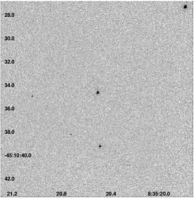
Figure 1: NUV-MAMA image with the Vela pulsar at center.

A direct 15 pixel (=$0\farcs 367$) radius aperture extraction of the pulsar gives 5650$\pm$84 counts. The F25SRF2 filter PSF is not tabulated in the STIS handbook, but measurement shows (Proffitt et al. 2002) that it is nearly identical to that of the F25QTZ filter, whose profile we obtain from the STIS handbook, Table 14.16. Correcting for the aperture losses gives a net pulsar signal of 6464$\pm$96 counts or 1.086$\pm$0.016 counts/s. The SRF2 filter has a central wavelength of 2270Å  and a 1/2 power range of 1900-3000 Å (with some response over 1300-3200 Å). Using the NUV MAMA/SRF2 effective areas from the STIS handbook Table 14.17, this countrate corresponds to $6.18\pm 0.09\times 10^{-18}{\rm erg\,cm^{-2}s^{-1}\AA^{-1}}$ (1.13$\pm$0.02 $\mu$Jy).

Choice of the best aperture for extraction of the pulsar signal is somewhat subtle. The large 15 pixel aperture provides a good estimate of the phase-averaged (DC) pulsar flux, but even this contains only 0.874 of the light of a well-centered PSF. Near pulse minimum, the flux is only a few percent of maximum. Here the measurement is background limited, rather than count limited, so a smaller aperture is preferred. Moreover, this background is time-variable. These factors imply that a time- and phase-dependent optimal (PSF-weighted) extraction is needed to obtain the best pulsar S/N, especially for the faintest portions of the light curve. So while we adopt aperture extraction for phase averaged values, optimal extraction is used for the time-resolved studies. We describe this extraction in §2.3.

Figure 2: FUV-MAMA background rates through the second orbit. The rates are counts per y (spatial) pixel per second. All fluxes are from a 100 pixel wide aperture flanking the Vela pulsar. Ly$\alpha$ and OI fluxes are integrated through the line, while the thermal count rate is measured from a line-free region covering spectral pixel range $425<x<800$.

For the FUV-MAMA spectroscopy, background is even more important. In particular the strong geocoronal Ly$\alpha$ and OI 1304 lines dominate the spectrum and vary strongly through the orbit. The OI] 1356 line is detectable, but not strong in these data. The 0$\farcs$5=20.5pix slit width projects to 11Å. We can choose spectral apertures to partly avoid these features, however the scattered line flux extends through an appreciable portion of the spectrum. Ly$\alpha$ is, for example, the dominant background over 1180Å -1245Å . In addition there is a strong and variable background from the thermal glow (Landsman, 1998). Our observations were made post-servicing mission SM3a, and the substantial detector temperatures caused a large background count rate. We minimized this background by offsetting the pulsar along the slit to a position with more modest thermal count rates (y$\sim 105{\rm pixel}\times 0\farcs 0244{\rm/pixel}=2\farcs 56$ from the bottom of the detector). The large (factor $\gtrsim 10$) variations in the geocoronal and thermal backgrounds are shown in Figure 2. For an initial characterization of the FUV spectrum, we selected 16 wavelength bands avoiding the bright geocoronal lines. Fluxes were obtained from an 11 pixel wide extraction box, whose centroid followed the expected y-position of the source. Backgrounds were extracted from 10-pixel wide strips offset 20 pixels above and below the pulsar. Each photon is weighted by the inverse of the normalized flat field $F_{ij}$ at the detector position $(i,j)$. Summing counts over the spatial aperture and wavelength bin, the source and background bin counts become $C=\Sigma C_{ij}/F_{ij}$. For each wavelength bin, we integrate the telescope response $R_{\lambda}$ (as a fraction of the unobscured HST aperture $A_{HST}$), the slit loss factor $T_{\lambda}$, the correction for the finite extraction aperture $H_{\lambda}$, and the time-dependent sensitivity factor $Q_{\lambda}$ to obtain the corresponding energy flux:

$$F_{\lambda}=\left({{hc}\over{A_{HST}}}\right){{C_{\rm net}}\over{\int R_{\lambda}T_{\lambda}H_{\lambda}Q_{\lambda}\lambda{\rm d}\lambda}}$$

These steps follow the standard calibration procedures generally applied to the phase averaged image as described in the HST STIS data Handbook (§3), but allow us to apply corrections to individual photons, preserving the pulsar phase information for further analysis. The resulting phase averaged flux spectrum is shown in Figure 3. The relatively large flux errors are caused by the strong background corrections that need to be applied to our fixed-width extraction aperture. Given that this background is highly variable, we will clearly want to go beyond simple aperture extraction when investigating the phase resolved spectrum.

Figure 3: FUV-MAMA aperture extracted, phase averaged spectrum.

2.3 Optimal Extraction of the Pulsar Signal

When the response of a detector, the noise properties of the observation and the detector location of the source PSF are known a priori, then, in principle, each detected photon in a given observation time gives an estimate of the source flux. The HST instruments have relatively stable and well characterized PSFs, and we can use off-source measurements to constrain the background; accordingly, we may use a weighted combination of the observed counts to make the best possible measurements of the pulsar spectrum, pulse profile and phase-resolved variations. The classic astronomical approach is optimal extraction (e.g. Naylor 1998). There are some special features of our application. First, our background varies both temporally and spatially (i.e. spectrally). Second, we need to define a weight for each photon, so that we can preserve arrival time phase. Happily, the significant temporal background variation is on a timescale $\gtrsim 100$ s, much longer than the pulse period. Thus our basic philosophy is to compute an optimal extraction weight for each position in $100$ s fiducial time chunks. In practice, we compute the weight for each event actually detected in the extraction window.

The background is used in two ways in the analysis. First, we need to subtract the background from the optimally weighted source spectrum. For this we use windows flanking the source extraction region, with a total area similar to the central extraction, and measured an average background per pixel $B(x,t)$. We also need a statistically independent estimate of the background and its temporal variation to use in computing the optimal extraction weights. This $B_{w}(x,t)$, measured from regions flanking the actual background, needs to be non-zero. As our Poisson data is fairly sparse, we replace zero backgrounds with the median counts/pixel in the line-free region when assembling this weighting factor.

HST calibration data give an estimate of the normalized spatial PSF $P_{xy}=P(\delta x,\delta y)$ where $\int P(\delta x,\delta y){\rm d}\delta x{\rm d}\delta y\equiv 1$. For the NUV channel, we use a simple radially symmetric PSF $P(r)$ for the F25QRTZ filter from the STIS handbook (this is nearly identical to the F25SRF2 PSF; see Proffitt et al. 2002). For the FUV channel the spatial PSF was available for three different $x$ (wavelengths) for the G140L, which we interpolated to get $P(x,\delta y)$. Standard extraction provided a good tracing of the pulsar spectrum central line $y(x)$, so we have $P_{xy}$, normalized at each $x$ along the spectrum. Since we will be treating very low S/N data we will only be following the spectrum in bins much coarser than the wavelength resolution, so we do not need to model the spectral extent of the PSF.

As above, we also can account for the (position dependent) sensitivity of the detector. For the imaging NUV channel, this is simply a flatfield correction, $S_{xy}=F_{xy}$. For the FUV spectral data we additionally include the wavelength dependent effective area $R_{x}$, the slit losses $T_{x}$ and the time-dependent sensitivity correction $Q_{x}$ (which is spectrally variable): $S_{xy}=F_{xy}*R_{x}*T_{x}*Q_{x}$.

With these definitions, we may ‘optimally extract’ the pulsar signal from the varying noise. Then we can extract the desired source counts $C$ from the data $D_{xy}$:

$$C=\sum_{xyt}W_{xy}(t)[D_{xy}(t)-B(t)],$$

where the sum is over some range ${x,y}$ corresponding to the pulsar source or to a wavelength bin, and the time dependent background/pixel $B(t)$ is corrected for the detector response $S_{xy}$ and averaged over the appropriate ${x,y}$ range at time $t$. Here

$$W_{xy}(t)=P_{xy}S_{xy}[P_{xy}*S_{xy}*C^{\prime}+B_{w}(t)]^{-1}N^{-1}$$

is the source photon weight at $(x,y,t)$ and

$$N=\sum_{xyt}P^{2}_{xy}S^{2}_{xy}[P_{xy}*S_{xy}*C^{\prime}+B_{w}(t)]^{-1}$$

is the weight normalization.

If one has a perfectly known PSF $P_{xy}$, detector sensitivity correction $S_{xy}$ and background model $B(x,y,t)$, then one uses a trial value for the source counts $C^{\prime}$, solves for $C$ and iterates to convergence. We find convergence in $\leq 3$ iterations. For the FUV observations the converged phase average spectrum is in good agreement with (but has smaller errors than) the aperture extracted spectrum. In the NUV, the 2-D PSF causes greater sensitivity to PSF shape and centering, and small differences in the average countrate remain after convergence. Accordingly, we re-normalize the total NUV flux to the aperture extraction value, but use the optimal extraction weights $W_{xyt}$ to form the highest S/N light curve.

For example an optimal extraction of the Vela NUV signal gives a 60-bin light curve with an average $\chi^{2}$ departure from constant of 17. The best simple aperture extraction (4 pixel radius) produces $\langle\chi^{2}\rangle$ = 15. Of course, the large (15 pixel radius) aperture used for the phase-averaged flux measurement contains too much background at pulse minimum, giving a rather poor $\langle\chi^{2}\rangle\sim 5$. Thus optimal extraction provides the best light curve S/N with a weighted combination of the source photons. Because small residual PSF and centering errors can affect the normalization, we adopt a hybrid approach in our measurement, taking the individual photon optimal weights and applying a small global renormalization to match the large aperture total counts.

A similar weighting applies for the FUV channel, although the extent of the sum $\sum_{xy}$ depends on the desired product. Phase resolved spectra in coarse wavelength bins will employ modest ranges of $\Delta x$ (which exclude the geocoronal emission lines). A simple FUV light curve would employ a summation over all $x$, $\delta y$ and $t$, weighting the low-noise, low-background time and wavelength slices highly in determining the weighted flux as a function of pulse phase. Note that to appropriately compute weight for counts in the FUV range, one needs a pre-existing estimate of the FUV pulsar spectrum.

Figure 4: NUV and FUV light curves from optimal extractions. Two periods are shown for clarity; an example error flag is shown in the second cycle. The lack of a flat minimum suggests that non-thermal emission contributes to all phases. The dotted lines show the phases of the 5 pulse components discussed by Harding et al. (2002). In the NUV panel the 4 pulse phase intervals and 3 off-pulse intervals discussed in the text are shown. The radio peak is at phase $\phi=0$.

3 Results

3.1 Pulsar Light Curve

We show the pulse profiles for the two UV channels in Figure 4. For the NUV data we show a 120 bin (0.74ms/bin) light curve; the noisier FUV data are plotted with 60 phase bins. Because of the limited absolute timing information in HST STIS data, the phases of these light curves relative to the radio are not independently determined. However we do see peak structures that correspond well to those seen in the optical and hard X-ray (RXTE) bands. Comparing with these, we estimate that the radio phase 0 is determined within $\sim\delta\phi<0.02$ (i.e. $\sim$2 ms uncertainty).

Several new features are seen for the first time in these data. First, as for the Crab pulsar, there is clearly non-thermal emission (presumably magnetospheric) at all phases, since no flat minimum appears in the light curve. Second, there are at least 4 distinct pulse peaks in the NUV band. Peaks 3 and 4 can be seen in the optical, but were first clearly identified in hard X-ray RXTE data by Harding et al. (2002). In our UV data these components show much more clearly and, in the higher resolution NUV light curve, we see that they are quite narrow. In particular P4, the pulse nearest in phase to the radio peak, appears unresolved in the NUV data. There is also clear structure in the main two peaks, seen here for the first time. The sharp peak in the $P2_{S}$ component is statistically significant in the NUV data and has a FWHM no larger than 1ms. This sharp structure is nearly coincident with, but much narrower than, the soft non-thermal component of the X-ray peak (P2_S). The broader UV component fills in the phase between the P2 soft and hard X-ray peaks. The latter peak $P2_{H}$ is prominent at GeV energies. The first UV peak, $P1_{S}$ lies near the optical peak and is clearly resolved. The UV data suggest that it is bifurcated, but improved count statistics will be needed to study such structure. As previously suggested in the optical light curve of Gouiffes (1998), the pulsed emission trails off following both P1_S and P2_S. The minimum emission is reached during phases $0.05<\phi<0.15$, our O2 off pulse interval. Interestingly, this interval includes the first (brightest) $\gamma$-ray pulse peak.

3.2 Phase-Resolved Spectra

The phase-average spectrum is a rather poor fit to a power law, with a substantial excess in the shortest wavelength bins. We should therefore not be surprised that the pulse components show a range of hardness. Our FUV statistics do not suffice to provide detailed phase-resolved spectra of all components of this complex pulse. However, we can examine the bright peaks in 4 coarse wavelength bins (avoiding the geocoronal lines). Figure 5 and Table 1 give the NUV+FUV phase-resolved fits to several components. Here the power law is $F_{\nu}=F_{0}(\nu/\nu_{0})^{-\alpha}$, where $F_{0}$ is the spectral flux value at $\nu=\nu_{0}=2\times 10^{15}$ Hz.

In these data we see that while the errors are large, it is clear that the $P1_{S}$ and $P2_{S}$ components are softer than $P3$. The O3 interval, which includes the tail of P2, is poorly represented by a power law, but in fact contains the highest 1170 Å count rate, making it relatively hard. The pulse minimum (O1&O2 intervals) is in contrast relatively flat with little FUV excess.

Table 1: Fits to Component Spectra [For E(B$-$V)=0.05]

Component	$\phi$	$\alpha$	Log[$F_{0}$($\mu$Jy)]
$P1_{S}$	0.21-0.35	$-$0.37$\pm$0.21	$-$0.52$\pm$0.03
$P2_{S}$	0.46-0.57	$-$0.22$\pm$0.13	$-$0.43$\pm$0.02
$P3$	0.86-0.90	0.45$\pm$0.06	$-$1.14$\pm$0.01
$P4$	0.00-0.04	$-$0.30$\pm$0.63	$-$1.23$\pm$0.08
${\rm O}1$	0.06-0.174	$-$0.10$\pm 0.19^{\dagger}$	$-$0.94$\pm$0.02†
${\rm O}2$	0.91-1.04	$-$0.10$\pm 0.19^{\dagger}$	$-$0.94$\pm$0.02†
${\rm O}3$	0.57-0.86	0.20$\pm$0.39	$-$0.43$\pm$0.05

^† Fit for the ‘Off’ = combined O1 and O2 intervals

Figure 5: NUV/FUV phase-resolved spectra. The observed fluxes are corrected here for an absorption E(B$-$V)=0.05. Best fit power laws are shown for the three brightest pulse peaks (solid lines). An upper limit to the Rayleigh-Jeans ($\nu^{2}$) flux present at pulse minimum is shown with the dashed line.

4 Discussion and Conclusions

Our data have shown that in the UV, the Vela pulse profile is dominated by multi-component non-thermal emission. To place this pulse in context, we show in Figure 6 the optical, NUV, hard X-ray and $\gamma$-ray light curves. In agreement with Harding et al. (2002) we find that there are at least five components in the non-thermal pulse profile. The two $\gamma$-ray peaks ($P1_{H}$ and $P2_{H}$) are lost below X-ray energies. In the FUV, these are replaced by $P1_{S}$ and $P2_{S}$ which continue to the optical. However, we find that $P2_{S}$ is structured, with a softer, narrow ‘spike’ on the leading edge and a relatively hard component extending into the O3 component. In fact, the soft spike corresponds best to the soft X-ray component of Harding et al. (2002), while our $P2_{S}$ may contain some of the hard component, extending into the $O3$ interval.

Figure 6: EGRET (Kanbach et al., 1994), RXTE (Harding et al., 2002) and optical (Gouiffes, 1998) light curves plotted with phase 0 set to the peak of the radio profile.

In addition to the narrow spike in $P2$, the peaks $P3$ and $P4$ are here seen to be very sharp. $P4$ is particularly interesting as it is close to the radio pulse phase and appears unresolved. For our approximate phasing, which is set by component matching to the optical and RXTE light curves, the $P4$ component trails the radio maximum by $\sim 1$ms. Interestingly, this is near the middle of the double peak radio pulse profile measured by Johnston et al. (2001), if the intermittent component seen by these authors is the trailing edge of a hollow cone. This might allow the $P4$ component to be produced by Compton up-scatter of radio photons from the center of the polar cap. However, given the uncertainty of the absolute UV pulse phase, it is equally plausible to associate this narrow component with the strong ‘$\mu$-Giant’ pulses (Johnston et al., 2001) that lead the main Vela radio pulse by $\sim 1.5$ms. This is attractive since true Giant pulse emission has been associated with narrow non-thermal components at high energy (Romani & Johnston, 2001). Given the recent demise of STIS, the best hope for testing this idea lies with high statistics optical light curves with good absolute phasing.

The physical origin of the various pulse components is presently unclear. In the outer magnetosphere picture of Romani (1996), the $\gamma$-ray peaks are argued to arise from caustics generated at the boundary of the open zone, well above the null charge surface. The lower energy emission with $P1_{S}$ and $P2_{S}$ converging from the X-ray through optical is then lower altitude emission with the radiation zone approaching the null charge surface. In the extended slot gap ‘two pole’ model described in Dyks, Harding & Rudak (2004) emission extends below the null charge surface and emission is visible from both poles. This wider range of possible emission zones may make it easier to understand the variety of pulse components seen for Vela. The hard, narrow component $P3$ is perhaps the most difficult component to understand, as it disappears at hard X-ray energies. Although quantitative predictions are not available, we suggest that this peak may be associated with inward-directed radiation from the same narrow magnetospheric gaps producing the outward-going, high energy radiation (Cheng, Ruderman & Zhang, 2000). In this case only relatively low energy photons can avoid pair production and traverse the magnetosphere to produce a pulse peak.

Figure 7: Phase-integrated spectrum from the IR through X-ray. We plot our UV phase-integrated fluxes (error flags include an estimated 5% flux calibration uncertainties) along with IR/optical points from Shibanov et al. (2003) and Mignani & Caraveo (2001) (circles). The model plotted is a H neutron star atmosphere fit to the Chandra data (NSA, long-dash line) along with a power law. Also shown is the range allowed for a power law fit to the 2.5-20 keV RXTE phase average spectrum. Our pulse minimum spectrum is plotted as a DC, unpulsed component (crosses) along with our upper limit to the Rayleigh-Jeans flux at pulse minimum (dot-dash line). This line, the DC equivalent of the RJ limit in Figure 5, lies below the NSA model (long-dashed line). The curved dotted line shows our upper limit with an added $\nu^{-0.5}$ power law.

We also wish to compare our spectrum with emission at other wavelengths. Figure 7 shows the IR-X-ray region of the Vela spectrum, which is dominated by thermal soft X-ray emission. Phase-averaged IR and optical fluxes from Shibanov et al. (2003), 555W, B and U fluxes from Mignani & Caraveo (2001) and our phase averaged NUV/FUV fluxes, all corrected for a reddening of E(B$-$V)=0.05, are plotted as open circles. Crudely the IR-UV data show a flat, $\alpha\approx 0$ spectrum. The ground-based U and our NUV point seem somewhat discrepant, but we suspect that these departures are artifacts of imperfect calibration. To compare with the X-rays, we plot a two component fit to the Chandra ACIS-S3 + HRC/LETG data (thick full line). This model has a magnetic H neutron star atmosphere component (NSA, Pavlov et al. 1995) with effective temperature $T_{\infty}=0.68\pm 0.01$ MK and radius $R_{\infty}=14.2\pm 0.5$ km at a distance of 300 pc (long dashed line) and a power law component with $\alpha=-1.08\pm 0.08$. A second thermal (i.e. hot polar cap) component is allowed, but not demanded by the fits. The soft Chandra power law clearly must break before the UV, as it extends well above the flat IR-UV spectrum. We also show the $\alpha=-0.41\pm 0.09$ power law that best fits the 2.5-20 keV phase-averaged RXTE data, and its uncertainty range. As noted by Shibanov et al. (2003), this extends to encompass the optical/IR points, but again there must be a break to $\alpha\approx 0$ in the UV range. The individual component spectral indices (Table 1) do not match the RXTE components measured by Harding et al. (2002), but given the evidence for a spectral break, the difference in phase structure between the UV and X-ray and the large errors in the UV spectral indices, this is not very surprising.

One of our original goals in this observation was to detect or limit the Rayleigh-Jeans (R-J) portion of Vela’s thermal surface spectrum. This will of course be most strongly constrained at pulse minimum. In Figure 7, we plot as crosses the pulse minimum (O$1$+O$2$) spectrum flux when this is an underlying DC (i.e. isotropic) component, after correcting for an assumed absorption E(B$-$V)=0.05. Clearly the strongest constraint on a R-J component comes from the highest frequency FUV points. Interestingly, these lie below the extrapolation of the NSA model in the two-component Chandra fit described above.

Even at pulse minimum the flux is largely non-thermal and the maximum R-J contribution depends on what is assumed for this non-thermal spectrum. If we assume an $\alpha=-0.5$ power law (PL) contribution, the steepest power law consistent with the RXTE spectrum, we obtain a limit of $6.25\nu_{16}^{2}\mu$Jy for the R-J component. This is shown as the dot-dash line in Figure 7, while the combined PL+R-J spectrum is shown as a curved dotted line. If instead a flat $\alpha\approx 0$ non-thermal component is assumed, the maximal R-J contribution is about 20% smaller.

In addition to the uncertainties associated with the non-thermal contribution at this phase, there is also uncertainty associated with the poorly known extinction. The Chandra X-ray fit has an absorption column $N_{H}=2.4\pm 0.2\times 10^{20}{\rm cm^{-2}}$. With a standard conversion $N_{H}\approx 2\times 10^{21}A_{V}\approx 6\times 10^{21}{\rm E(B-V)}$, this gives an estimate E(B$-$V) =$0.04\pm 0.003$ for Vela’s reddening. This is consistent with line ratios measured for nearby Vela remnant filaments (Wallerstein & Balick, 1990), although some filaments show reddening estimates as large as E(B$-$V)=0.1. For this larger extinction, the phase integrated spectrum has an abrupt jump in the NUV, with a peak flux of $\sim 2.7\mu$Jy at $\sim 2000$ Å, a factor of 1.7$\times$ higher than the IR-optical flux, followed by a decrease in the FUV. This would be of appreciable interest for interpretation of the non-thermal emission, but seems less plausible than a simple uniform spectrum. Thus, our adopted E(B$-$V) = 0.05 represents a reasonable estimate for the extinction at the pulsar’s position, although larger values cannot be ruled out.

As a final caveat, it is important to note here that the UV light curve of Geminga measured by Kargaltsev et al. (2005) shows an eclipse-like minimum. This minimum was interpreted as the effect of magnetospheric scattering, which can remove thermal surface flux from a window of pulse phase near the polar cap. Clearly, if such scattering occurs for Vela, the pulse minimum could be suppressed, and we would infer an unrealistically low Rayleigh-Jeans temperature. However, both the O1 and O2 minima have comparable fluxes and seem to lie near the asymptotic value extrapolated from the O3 window (see Fig. 4). Thus, a rather special scattering geometry would be needed to suppress the O1/O2 flux without showing up in the light curve. Also, a rather abrupt break in the non-thermal contribution at $\sim 2\times 10^{15}$Hz would be needed to permit a R-J component comparable to the total flux in the shortest wavelength FUV bins (see Fig. 5). Accordingly, we take the $6.25\nu_{16}^{2}\mu$Jy limit above as fairly conservative, and for a $13R_{13}$ km neutron star at $300d_{300}$pc we obtain

$$T_{\rm RJ}\leq 3.3\times 10^{5}{\rm K}(d_{300}/R_{13})^{2}10^{0.4A_{1210}[{\rm E(B-V)}-0.05]},$$

where the last term with $A_{1210}\approx 10$ highlights the dependence on the imprecisely known extinction.

At $d=300$ pc, the Chandra NSA fit gives $T\,R^{2}=137{\rm MK\,km^{2}}$. However, a light element atmosphere has a Wien excess and, correspondingly, a R-J depression when compared with the Planck spectrum at the same $T_{\rm eff}$. In fact, the NSA model above has a flux corresponding to $80{\rm MK\,km^{2}}$ in the R-J regime. This is, however, still 45% larger than the $55{\rm MK\,km^{2}}$ from our pulse minimum flux. Correcting for a rather high extinction E(B$-$V)$\geq 0.1$ would make the FUV flux just consistent with the NSA model, but at the cost of introducing a peak in the phase-integrated non-thermal spectrum, as noted above. There is a precedent for observed UV flux levels below the extrapolation of the best-fit X-ray thermal spectrum. Our FUV observations of the Geminga pulsar (Kargaltsev et al., 2005) clearly detect the $\nu^{2}$ R-J surface component at $0.45-0.55R_{13}^{-2}$ MK; this is again below the R-J extrapolation of the X-ray fit. Detailed interpretation of these UV fluxes will require improved models of the opacity in this band from low temperature neutron star surfaces. However, we may generally infer that the R-J emission gives a better indicator of the average surface temperature, since the X-ray Wien tail can be boosted by unmodeled hot spots and non-thermal components.

Thus, with the caveats above in mind, we interpret our measurement as supporting a very low surface temperature for the young $\tau_{c}\approx 10^{4}$yr Vela pulsar. Even if E(B$-$V) is increased to 0.1 to match the X-ray fit predictions, the best-fit X-ray surface temperature of 0.68 MK at R= 14.2 km is already below standard cooling predictions for such a young neutron star (Tsuruta et al., 2002; Yakovlev & Pethick, 2004), implying the existence of enhanced neutrino emission, e.g. due to kaon core condensates. The non-thermal spectrum then has a peak in the near-UV. If, on the other hand, our E(B$-$V)$\approx$0.05 estimate of extinction to the pulsar is supported by further studies, the effective surface temperature is significantly lower, having important implications for the high density equation of state (EOS) and conditions in the neutron star core. The 0.33 MK value for blackbody emission from a canonical 13 km star would rule out all but the fastest cooling models. More realistically, if we adopt the $R=14.2$ km of the X-ray fit and the $T_{RJ}=0.59T_{\rm eff}$ RJ suppression of the NSA model, we infer an effective temperature limit $T_{\rm eff}\leq 0.46$ MK. This is quite cool compared to other young neutron stars. This temperature would imply that Vela is a high mass neutron star with rather weak suppression of the URCA process. It would appear that the softest EOS can now be excluded, since such rapid cooling favors core pion condensates or even core hyperon matter (Yakovlev & Pethick, 2004). Further, models which reach such low temperatures by $10^{4}$yr for these EOS generally do not have strong core proton superfluidity; the minimum required mass is $\approx 1.6-1.7M_{\odot}$, depending on the EOS. Thus, this low Vela $T_{RJ}$ provides some of the strongest available constraints on matter at high density. Such an important result certainly argues for further study and confirming observations.

References

- Cheng, Ruderman & Zhang (2000) Cheng, K.S., Ruderman, M. & Zhang, L. 2000, ApJ, 537, 964
- Dyks, Harding & Rudak (2004) Dyks, J., Harding, A.K. & Rudak, B. 2004, ApJ, 606, 1125
- Gouiffes (1998) Gouiffes, C. 1998, in Neutron stars and Pulsars, ed. N. Shibazaki, N. Kawai, S. Shibata, & T. Kifune (Tokyo:Univ. Acad. Press), 363.
- Harding et al. (2002) Harding, A.K. et al. 2002, ApJ, 576, 376
- Johnston et al. (2001) Johnston, S. et al. 2001, ApJ, 549, L101
- Kanbach et al. (1994) Kanbach, G. et al. 1994, A&A, 289, 855
- Kargaltsev et al. (2005) Kargaltsev, O.Y., Pavlov, G.G., Zavlin, V.E. & Romani, R.W. 2005, ApJ, in press
- Landsman (1998) Landsman, W. 1998, Characteristics of the FUV-MAMA Dark Rate, STIS IDT report
- Mignani & Caraveo (2001) Mignani, R.P & Caraveo, P.A. 2001, A&A, 376, 213
- Naylor (1998) Naylor, T. 1998, MNRAS, 296, 339
- Pavlov et al. (1995) Pavlov, G. G, Shibanov, Y. A., Zavlin, V. E., & Meyer, R. D. 1995, in The Lives of the Neutron Stars, eds. M.A. Alpar, U. Kiziloglu, J. van Paradijs (Kluwer: Dordrecht), 71
- Proffitt, et al. (2002) Proffitt, C.R., Davies, J.E., Brown, T.M. & Mobasher, B. 2002, in 2002 HST Calibration Workshop, S.Arribas, A. Koekemoer and B. Whitmore, eds., p. 201
- Romani (1987) Romani, R.W. 1987, ApJ, 313, 718
- Romani (1996) Romani, R.W. 1996, ApJ, 470, 469
- Romani & Johnston (2001) Romani, R.W. & Johnston, S. 2001, ApJ, 557, L93
- Sanwal et al. (2002) Sanwal, D. et al. 2002, in Neutron Stars in Supernova Remnants, ASP Conf., 271, 353
- Shibanov et al. (2003) Shibanov, Yu.A., Koptsevich, A.B., Sollerman,J. & Lundquist, P. 2003, A&A, 406, 645
- Tsuruta et al. (2002) Tsuruta, S. et al. 2002, ApJ, 571, L143
- Wallerstein & Balick (1990) Wallerstein, G. & Balick, B. 1990, MNRAS, 245, 701.
- Yakovlev & Pethick (2004) Yakovlev, D.G. & Pethick, C.J. 2004, Ann. Rev. Astron. Astrophys., 42, 169
- Zavlin & Pavlov (2002) Zavlin, V.E. & Pavlov, G.G. 2002, in Neutron Stars, Pulsars and Supernova Remnants, Proc. of the 207th Heraeus Seminar, ed. W. Becker, H. Lesch and J. Trum̈per (MPE Report 278), astro-ph/0206025