CMB Polarimetry using Correlation Receivers with the PIQUE and CAPMAP Experiments

Abstract

The Princeton IQU Experiment (PIQUE) and the Cosmic Anisotropy Polarization MAPper (CAPMAP) are experiments designed to measure the polarization of the Cosmic Microwave Background (CMB) on sub-degree scales in an area within $1^{\circ}$ of the North Celestial Pole using heterodyne correlation polarimeters and off-axis telescopes located in central New Jersey. PIQUE produced the tightest limit on the CMB polarization prior to its detection by DASI, while CAPMAP has recently detected polarization at $\ell\sim 1000$. The experimental methods and instrumentation for these two projects are described in detail with emphasis on the particular challenges involved in measuring the tiny polarized component of the CMB.

1 INTRODUCTION

The polarized component of the Cosmic Microwave Background (CMB) provides abundant information about the structure and dynamics of the early universe. Measurements of the E-mode polarization complement temperature anisotropy observations, and the consistency between these data sets should provide strong confirmation of the standard hot Big Bang cosmology. Measurements of the B-mode polarization can both reveal gravitational lensing of the CMB (Zaldarriaga & Seljak, 1998; Seljak & Hirata, 2004; Smith et al., 2004) and probe the gravity wave content of the universe (Seljak & Zaldarriaga, 1997, 1999; Kamionkowski & Kosowsky, 1998). Recently, a polarized component of the CMB was detected by the DASI (Kovac et al., 2002; Leitch et al., 2002) and WMAP (Bennett et al., 2003a) experiments. These early data were extended last year by new results from CAPMAP (Barkats et al., 2004), DASI (Leitch et al., 2004), and CBI (Readhead et al., 2004). Now about a dozen experiments are underway to characterize this elusive signal. These various projects employ a variety of detection techniques to contend with the small size of the polarized signal (a few $\mu$K rms), which demands not only high sensitivity but also stringent control of systematic effects.

This paper describes the experimental methods and instrumentation for the Princeton IQU Experiment (PIQUE) and the Cosmic Anisotropy Polarization MAPper (CAPMAP), both of which have used correlation polarimetry at 90 and 40 GHz and off-axis telescopes to search for the E-mode polarization of the CMB. The PIQUE and CAPMAP instruments have been described briefly in their respective results papers (Hedman et al., 2001, 2002; Barkats et al., 2004). Here we give a detailed description of their characterization and optimization, with emphasis on both unexpected challenges met and new techniques developed which will be relevant for future large-scale experiments. Further discussion on specific topics may be found in Hedman (2002) and Barkats (2004). After an overview of the projects (§ 2) and the Stokes parameters in the context of CMB observations (§ 3), we describe the polarimeters (§ 4) and the optics for the two experiments (§ 5), as well as the atmospheric characteristics of the observing sites (§ 6). We conclude with detailed discussions on the operation, performance, and calibration of the instruments (§ 7), with a special focus on polarization-specific systematic effects (§ 8), including those that—although small enough to be neglected in these experiments–will prove crucial for future campaigns.

Table 1 summarizes the acronyms used throughout this paper.

2 OVERVIEW

A summary of the main characteristics of the PIQUE and CAPMAP systems is provided in Table 2.

PIQUE consisted of two independent heterodyne correlation polarimeters using cryogenic high electron mobility transistor (HEMT) amplifiers coupled through corrugated feed horns to a 1.2-meter off-axis parabolic primary mirror. One polarimeter operated at W-band (84–100 GHz) with a nearly Gaussian, $15\arcmin$ full width at half maximum (FWHM) beam. The other operated at Q-band (35–45 GHz) with a $30\arcmin$ FWHM beam. Construction of the PIQUE instrument began in 1997, and observations were made from the roof of Jadwin Hall in Princeton, New Jersey on two successive winters in 2000 and 2001. Observations at W-band near the North Celestial Pole (NCP), published in Hedman et al. (2001, 2002), provided the tightest limits on the polarized component of the CMB prior to its detection by the DASI experiment (Kovac et al., 2002).

CAPMAP extends the fundamental technologies developed for PIQUE to smaller angular scales and higher sensitivity. The full CAPMAP instrument is an array of 16 polarimeters installed in the focal plane of the 7-meter antenna (Chu et al., 1978) at Lucent Technologies in Holmdel, NJ. Twelve of the polarimeters operate at W-band and four at Q-band. This combination provides nearly equal sensitivity at two frequencies and will allow galactic foregrounds to be identified and removed if needed. The beam FWHMs are $4\arcmin$ and $6\arcmin$ at W-band and Q-band, maximizing CAPMAP’s sensitivity to angular scales where the E-mode polarization is expected to peak ($\ell\sim 1000$). The CAPMAP instrument was designed to be fielded in a staged deployment. In the winter of 2002–2003, four W-band receivers (denoted $A$–$D$) in a single dewar made observations. The results from the first season of CAPMAP are published in Barkats et al. (2004). Twelve polarimeters in three dewars recorded data in the winter of 2003–2004, and analysis of these data is underway. The full CAPMAP system, with 16 polarimeters, has now been deployed for the winter of 2004–2005.

3 STOKES PARAMETERS

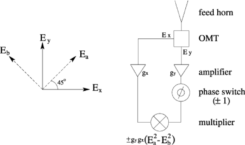
Figure 1: Principles of correlation polarimetry. The polarimeter couples the two orthogonal components of the incident electric field ($E_{x}$ and $E_{y}$) into separate arms. After amplification, both components are fed into a multiplier, which produces an output voltage proportional to the product of the two input fields. This product is proportional to the Stokes parameter $U=\left\langle 2E_{x}E_{y}\right\rangle=\left\langle E_{a}^{2}\right\rangle-\left\langle E_{b}^{2}\right\rangle$, where $E_{a}$ and $E_{b}$ are another set of orthogonal components of the radiation illustrated above. The signal from the correlation polarimeter can be modulated rapidly using a $0^{\circ}$–$180^{\circ}$ phase switch in one of the arms, which takes $U$ to $-U$. Fluctuations in the gains $g_{x}$ and $g_{y}$ alter only the small polarized component rather than the total intensity.

The Stokes parameters $I$, $Q$, $U$, and $V$ completely determine the polarization state of an electromagnetic wave, and they form the basic formalism of astronomical polarimetry (Hamaker et al., 1996; Kraus, 1986; Jackson, 1998). The CMB is not expected to have a circularly polarized component, so in what follows we consider the case $V=0$. The remaining parameters can be quantified using a particular coordinate system. Define two orthogonal axes $x$ and $y$ in the plane perpendicular to the incident wave vector. Next, define the orthogonal axes $a$ and $b$ which are rotated $45^{\circ}$ with respect to $x$ and $y$ as illustrated in Figure 1. The components of the electric field polarized along each of these axes are $E_{x}$, $E_{y}$, $E_{a}$, and $E_{b}$ such that $E_{x}=\frac{1}{\sqrt{2}}\left(E_{a}-E_{b}\right)$ and $E_{y}=\frac{1}{\sqrt{2}}\left(E_{a}+E_{b}\right)$. The Stokes parameters can then be written as

$$\begin{array}[]{ccccc}I&=&\left\langle E_{x}^{2}\right\rangle+\left\langle E_{y}^{2}\right\rangle&=&\left\langle E_{a}^{2}\right\rangle+\left\langle E_{b}^{2}\right\rangle,\\ Q&=&\left\langle E_{y}^{2}\right\rangle-\left\langle E_{x}^{2}\right\rangle&=&2\left\langle E_{a}E_{b}\right\rangle,\\ U&=&2\left\langle E_{x}E_{y}\right\rangle&=&\left\langle E_{a}^{2}\right\rangle-\left\langle E_{b}^{2}\right\rangle.\end{array}$$ (1)

The angle brackets denote a time average over the sampling period of the detector. The interpretation of the Stokes parameters in this basis is clear. The parameter $I$ is the total intensity of the radiation (up to a constant factor), while $Q$ and $U$ quantify the linear polarization. The polarization fraction $P=\sqrt{Q^{2}+U^{2}}/I$ and the polarization orientation $\theta=\frac{1}{2}\arctan(U/Q)$ can be derived from these parameters. The Stokes parameters provide a natural formalism for CMB polarimetry because the output of a polarimeter is generally proportional to some linear combination of $Q$ and $U$ (see Figure 1). However, this formalism also requires (1) that the parameters be defined self-consistently and (2) that a coordinate system be specified appropriately.

As defined in Equation 1, $I$, $Q$, and $U$ are self-consistent under transformations of the coordinate system and other operations on the state of the radiation field, which can be implemented using the Jones matrix or Mueller matrix formalism (Heiles et al., 2001; Tinbergen, 1996; O’dell, 2002). A similarly self-consistent set of parameters can be generated by multiplying all of these terms by the same constant factor. Thus we can generate Stokes parameters with units of temperature as follows: if $T_{x}$ is the physical temperature of a blackbody which emits the observed value of $\left\langle E_{x}^{2}\right\rangle$ (and similarly for $T_{y}$), then the Stokes parameters can be expressed as $I=\left(T_{x}+T_{y}\right)/2$ and $Q=\left(T_{x}-T_{y}\right)/2$. With this convention, $I$ is the temperature of the object which produces the observed unpolarized intensity, and $Q$ is the consistent measure of the linear polarization.

Two natural coordinate systems are typically used to define $Q$ and $U$ in astronomical polarimetry. One system, established by the IAU (1973), defines a coordinate system at every point in the sky such that a signal polarized parallel to a great arc connecting the celestial poles has positive $Q$ and zero $U$. This system is useful for combining and comparing measurements from different instruments, but for individual polarimeters there is also a coordinate system defined by the instrument itself. The latter is useful when discussing the performance and characteristics of the experiment and is used exclusively in this paper.

4 POLARIMETERS

The CAPMAP and PIQUE projects use phase-switched correlation polarimeters. Here we give an overview of correlation polarimetry followed by details of its implementation in PIQUE and CAPMAP.

4.1 Principles of Correlation Polarimetry

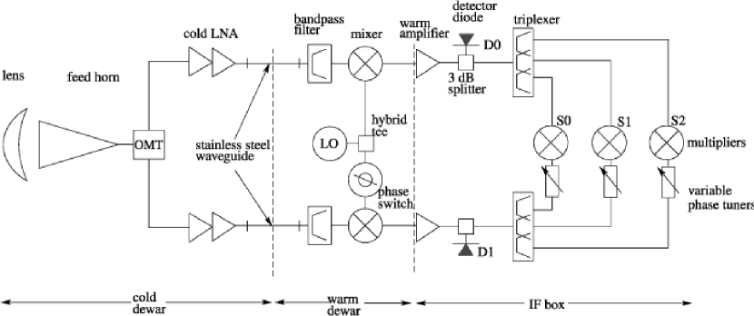
Figure 2: Block diagram of the PIQUE and CAPMAP polarimeters. In CAPMAP the components inside the dewar are either cryogenically cooled (cold dewar), or kept at room temperature (warm dewar). In PIQUE, the LO, phase switch, and hybrid tee were located outside the dewar while the filters and mixers were cooled to 50 K–80 K (see Table 5). After the mixers, the signals exit the dewar via coaxial cable and are further processed in the IF box. The IF box is an RF-tight enclosure, mechanically attached to the dewar. The three polarimetry channels are S0, S1, and S2, while the two total power (intensity) channels are D0 and D1. Refer to § 4.2 for a detailed description of the polarimeter.

Both PIQUE and CAPMAP use phase-switched correlation polarimeters to extract small polarized signals from largely unpolarized radiation. Figure 1 sketches the key details of such a polarimeter. It has two identical “arms”, each of which carries radiation coherently from an ortho-mode transducer (OMT) to a multiplier. The OMT defines a set of coordinate axes $x$ and $y$. The $x$ component of the incident electric field, $E_{x}$, is coupled through one output of the OMT into one arm of the polarimeter, while $E_{y}$ is coupled into the other arm. The two arms (see also Figure 2) contain devices which amplify and filter these components of the radiation before they reach the multiplier. The output voltage of the multiplier is proportional to the product $\left\langle E_{x}E_{y}\cos\theta\right\rangle$, where the angle brackets denote a low-pass-filtered time average, and $\theta$ is the phase difference between $E_{x}$ and $E_{y}$. In the case of $V=0$, this phase difference arises entirely from mismatches between the receiver arms. The output is proportional to the $U$ Stokes parameter in the instrumental coordinate system defined by the OMT. In contrast to the correlation polarimeters used in PIQUE and CAPMAP, a number of CMB polarization experiments use differencing polarimeters, which measure $\left\langle E_{x}^{2}\right\rangle$ and $\left\langle E_{y}^{2}\right\rangle$ separately and then difference to obtain an estimate of $Q$ (Johnson et al., 2003; Montroy et al., 2003; Keating et al., 2003; Church et al., 2003). Differencing polarimeters using bolometers from balloons and satellites can achieve better sensitivities than correlation polarimeters, which rely on coherent amplifiers. However, correlation polarimetry has advantages in the control of systematic effects. For both types of polarimeter there are coupling coefficients $c_{x,y}$ between the components of the electric field and the detector elements, so that the outputs of the polarimeters are:

$$2c_{x}c_{y}\left\langle E_{x}E_{y}\right\rangle$$ (2)

for a correlation system and

$$c_{x}^{2}\left\langle E_{x}^{2}\right\rangle-c_{y}^{2}\left\langle E_{y}^{2}\right\rangle$$ (3)

for a differencing polarimeter. The coupling coefficients will in general drift in time. If the radiation is unpolarized ($\langle E_{x}^{2}\rangle-\langle E_{y}^{2}\rangle=\langle E_{x}E_{y}\rangle=0$), these drifts do not generate a spurious nonzero output in a correlation polarimeter (to first order).

In practice, either type of polarimeter has a time-variable offset. The stability requirements on these offsets can be greatly reduced by modulating the input signal. If the signal is modulated at a frequency $f$, then only drifts in the offset on time scales shorter than $1/f$ are relevant. The phase switch in a correlation polarimeter multiplies the electric field in one arm by $\pm 1$ by adding alternately $0^{\circ}$ or $180^{\circ}$ of extra phase. This switching can be done at frequencies of a few kHz. The demodulated output of the correlation polarimeter is therefore immune to nearly all $1/f$ noise caused by gain drifts in the receiver.

4.2 Construction

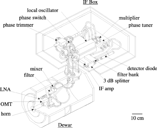
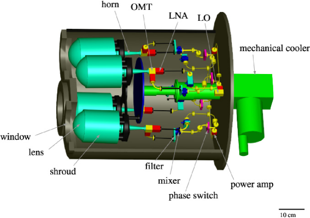
Figure 3: Cutaway drawings of the PIQUE (top) and CAPMAP (bottom) polarimeters. In CAPMAP, each receiver looks through its own 6 in (15.24 cm) diameter window, made of a 0.75 mil (19 $\micron$) layer of polypropylene backed with a 125 mil (3.127 mm) layer of Goretex (RA7957 from W. L. Gore). The single PIQUE 1 in (2.54 cm) diameter window consists of 2 mil (50 $\micron$) polypropylene and 20 mil (0.5 mm) Goretex. Above the horn of each CAPMAP receiver are the lens and lens shroud, described in more detail in § 5.2. Note that neither the thermal straps nor the wiring to the active devices is shown. The phase tuners in the IF section allow the path length in one arm to be adjusted to match that of the other arm. The box containing the IF section of the polarimeters is not shown in the CAPMAP system; it contains the same components as the PIQUE system in a more compact configuration.

Most of the heterodyne correlation polarimeters used in PIQUE and CAPMAP are sensitive to W-band radiation, where the contribution from astrophysical foregrounds is expected to be minimal (Tegmark et al., 2000). Q-band polarimeters provide data at a second frequency for foreground identification. The basic architecture of all of these instruments is essentially the same, so the following description focuses on the W-band polarimeters; the Q-band instruments are discussed only insofar as they differ from the W-band systems. Figures 2 and 3 illustrate the architecture of the PIQUE and CAPMAP polarimeters. The incident radiation is first coupled into the radio frequency (RF) section, where the first stage of amplification and bandpass filtering is performed. A mixer and local oscillator (LO) system introduces the 4 kHz phase modulation and down-converts the radiation in both arms to the intermediate frequency (IF) band at 2–18 GHz. This radiation enters the IF section where the signal is further amplified and divided by filter banks into three (for W-band) or two (for Q-band) frequency sub-bands. For each sub-band, an analog multiplier receives the radiation from both arms and produces an output voltage. The back-end electronics extract the component of this voltage modulated at 4 kHz, which is proportional to the $U$ Stokes parameter of the incident radiation. Finally, a data acquisition program stores the amplitude of the modulated signal to disk. The signal levels carried through each device are summarized in Table 3. A list of the actual components used in the polarimeters is provided in Table 4.

4.2.1 RF Section

Radiation enters the polarimeter through a feed horn (see § 5), and the OMT couples two orthogonal polarized components of the radiation into the two arms of the polarimeter via waveguide. The isolation between the outputs of the OMT is an important factor in determining the polarization fidelity of the polarimeter and is discussed at length in § 8.1.

Low-noise amplifiers (LNAs) are attached directly to both outputs of the OMT. Both PIQUE and CAPMAP use cryogenic amplifiers based on indium-phosphide (InP) HEMTs to achieve high gain with low noise. For PIQUE, the LNAs were designed by M. Pospieszalski for the WMAP satellite (Jarosik et al., 2003). While these components were acceptable LNAs, they were not available in large numbers because each amplifier was laboriously assembled from multiple individual HEMT devices by hand. CAPMAP’s LNAs use monolithic microwave integrated circuits (MMICs) made from InP HEMTs (Weinreb et al., 1999) designed at JPL and Northrop Grumman Corporation. MMIC technology circumvents the time-consuming and expensive assembly procedures and enables the large number of LNAs required by the CAPMAP experiment to be produced quickly, reproducibly, and at relatively low cost.

The OMTs, LNAs, and horns are cooled to cryogenic temperatures (25–40 K) with a closed cycle helium refrigerator (see § 4.2.5). Stainless steel waveguide provides the thermal break between these components and the remainder of the polarimeter, which operates at warmer temperatures. The rest of the RF section consists of various waveguide sections and a band-defining filter, followed by the mixer. In PIQUE, these components were cooled by the first stage of the refrigerator. In CAPMAP, these components were kept inside the dewar but operated at room temperature (see Table 5).

4.2.2 Mixer-LO System

The mixers require a narrow-band, high-power tone to down-convert the RF signal to the IF band. This signal is provided by the LO, which is coupled to both mixers via a waveguide hybrid tee and two waveguide paths. A phase switch in one path modulates the electric field at one mixer by $\pm 1$. The modulation frequency is 4 kHz, well above the $1/f$ knee of the polarimeter noise power spectrum, so that the raw polarimetry data are stable on time scales of many minutes (see § 7.2).

Both PIQUE and CAPMAP use baseband rather than harmonic mixers. The LO tones are therefore at a frequency comparable to the RF signals: 30.5 GHz for Q-band, 82 GHz for W-band. This imposes strong constraints on the LO system design, because the high-frequency signals can only be transmitted efficiently over rigid waveguide, and the two LO paths must have the same length to within a millimeter to insure optimal performance (see § 4.3.1). Furthermore, at 90 GHz the passive loss through waveguide is relatively high ($\sim 1.5$ dB/ft for warm Cu waveguide), and the RF power production efficiency is relatively low, making it more difficult to deliver the required power to the mixers.

In PIQUE, each polarimeter had a powerful 100 mW LO located outside the dewar. A portion of the LO section was therefore accessible for phase tuning when the dewar was closed. The drawback of this LO system was that it consisted of convoluted, several-foot-long paths of lossy waveguide (see Figure 3).

In the CAPMAP array, the entire mixer-LO system is contained in the dewars (see Figure 3) and uses smaller, lower power LOs along with external MMIC power amplifiers (Huei et al., 2001). Initially, each polarimeter had an independent LO for greater modularity. In this configuration, the outputs of the polarimeters had significant offsets that were extremely sensitive to mechanical vibrations. These offsets occurred because the proximity between the LO tone and the RF band made it possible for LO signals leaking out of the waveguide to couple optically into the RF sections of the polarimeters. Since the LOs were not locked to the same frequency, the tone leaking from one LO into other polarimeters was down-converted to a few hundred MHz at the output of the mixers, saturating the IF amplifiers.

This problem was greatly reduced by running all the W-band polarimeters in a dewar from a single LO, using power amplifiers to insure the delivery of sufficient power to each polarimeter (see Figure 3). However, the leaking LO tone could still degrade the performance of the polarimeter by saturating the LNAs, so all waveguide joints were covered in microwave absorber and aluminum tape, and a portion of the inside of the dewar was lined with absorber to control further leakage. These procedures have been followed in subsequent seasons of CAPMAP, where both Q-band and W-band polarimeters exist in a single dewar. (The third harmonic of the Q-band oscillator is in the middle of the W-band polarimeters’ RF band, so the leakage between these radiometers must also be controlled.)

4.2.3 IF Section

The IF sections of PIQUE and CAPMAP are virtually identical (except for the models of the IF amplifiers and phase tuners). After down-conversion, the 2–18 GHz signals are carried on semi-rigid SMA coaxial cables out of the dewar into an “IF box”. Here IF amplifiers provide additional gain before 3 dB splitters direct half the power in each arm to detector diodes, which measure the total power in the arm (defined as the D0 and D1 channels regardless of their orientation on the sky). The other half of the power enters a filter bank, which splits the radiation into three roughly equal IF bands corresponding to RF frequency bands of 84–89, 89–94.7, and 94.7–100 GHz for the W-band polarimeters. In the Q-band polarimeters they correspond to 35–40 and 40–45 GHz. The radiation from both arms of each of these sub-bands is fed into an analog multiplier. In front of each multiplier, a phase tuner allows the length of one arm of the polarimeter to be changed in order to match the phase length in each arm (see § 4.3.1). Each multiplier outputs a voltage proportional to the product of the two input fields (see § 4.1). The outputs of the multipliers for the three sub-bands are denoted S0, S1, and S2 in order of increasing frequency; S2 does not exist in the Q-band polarimeters.

4.2.4 Back-End Electronics/DAQ

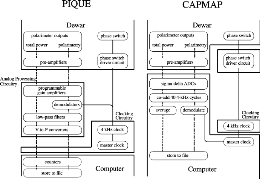
Figure 4: Block diagrams of the data acquisition systems of the PIQUE and CAPMAP experiments. These electronics provide the 4-kHz signal to the phase switch and synchronously demodulate the data from the polarimetry channels. In PIQUE these tasks were performed by custom-made, largely analog circuitry, while CAPMAP used commercial ADCs, with demodulation in software.

Both PIQUE and CAPMAP use pre-amplifiers to buffer and amplify by 100 the output voltages from the multipliers and detector diodes before they are transmitted to the processing electronics and the data acquisition system. These electronics are responsible for providing the clocking signal to the phase switch and for synchronously demodulating the polarimetry data for storage to disk. PIQUE and CAPMAP use different techniques to perform these two functions, as illustrated in Figure 4.

In PIQUE, a series of custom-made analog circuits demodulate, filter, and digitize the polarimeter output voltages before they are transmitted and stored on a computer. First, a programmable-gain amplifier circuit buffers and amplifies the signals from the pre-amps. Then the polarimetry channel data is demodulated using an analog circuit based on a modulator/demodulator chip. Finally, both the polarimetry and the total power channel signals are filtered before reaching a voltage-to-frequency ADC. The digital outputs of this circuit are then transmitted and stored to file on a PC running MS-DOS. The master clock for this system is a 4.096-MHz oscillator located outside the computer. This clock is divided by 1024 to 4 kHz, yielding the reference clock for the phase switch driving circuit and the demodulation circuit. This clock signal is also divided down to the 31.25-Hz sampling rate to provide interrupts to the data acquisition program.

In CAPMAP the output voltages from the pre-amps are transmitted directly to a PC running Linux, where they are digitized at 100 kHz by a commercial 24-bit sigma-delta ADC with 32 differential channels. This sampling rate yields 24 samples per 4-kHz cycle and can adequately record the 4-kHz square waves. These data are then digitally demodulated and down-sampled to 100 Hz in software before being recorded to file. In the first season, a second set of “raw”, undemodulated files was recorded containing averages of 40 4-kHz cycles for every channel. This digital demodulation enables a variety of “quadrature” demodulations to be implemented for systematic checks and debugging purposes. The master clock is a 12.8-MHz oscillator on the ADC, which is down-converted to 4 kHz in an external “clock box” before being sent to the phase switch driver circuitry. During the first CAPMAP observing season, although the 4-kHz clock was synchronized with the data acquisition and demodulation programs, the phase between these two clocks varied each time the acquisition program was restarted between observing sessions, so the data required additional off-line processing involving the raw files. The software and clock-box were upgraded for the subsequent observing season to eliminate this problem.

4.2.5 Radiometer Environment

Cryogenics

A closed-cycle refrigerator cools the LNAs, horns, and OMTs to cryogenic temperatures. For PIQUE the LNAs were attached to the second stage of the refrigerator, while the filters and mixers were attached to the first stage. During the first season of PIQUE, IF amplifiers were located inside the dewar, attached to the first stage of the refrigerator. This stage of amplification was unnecessary and was removed for the second season, which reduced the loading on the cold head and lowered the operating temperature of the other cryogenic components. Table 5 shows typical operating temperatures during the two observing seasons.

Performance of the polarimeters does not improve when the mixers and filters are cooled, so for CAPMAP it was decided to operate these components at room temperature inside the dewar. The LNAs operated at higher temperatures (see Table 5) than in PIQUE due to the increased thermal load on the refrigerator with four polarimeters and the larger windows which were required for the lenses (see § 5). Modifications to improve the thermal isolation between the cold stages have been completed and have reduced the LNA temperatures to between 20 K and 30 K for the CAPMAP 2004 season.

For PIQUE and the first season of CAPMAP, the dewars lacked thermal regulation, so the various components came to temperatures determined by the cooling power of the cold head. During the course of three months of observing, the temperature of the LNAs drifted by $\sim 3$ K. These drifts did not affect the gain of the polarimeters by more than a few percent (see § 7.2.1) and did not significantly affect the data quality. A system for thermal regulation was built into the CAPMAP dewars but was not activated until the 2004 season.

In both PIQUE and CAPMAP, the feeds look out of the dewar through polypropylene windows (see Figure 3). To prevent moisture in the air from condensing on these windows, another polypropylene sheet is used to create an isolated air space, which is kept dry using Drierite pellets. In PIQUE the pellets were placed in the dry space itself, while CAPMAP used a recirculating air system including a cylinder packed with Drierite.

Operational Configuration and Thermal Environment

For PIQUE the IF box containing the LO and the IF components was exposed to the outdoor environment. Most of the back-end electronics and associated power supplies were also located outside on the telescope base, while the DAQ computer and the compressor running the refrigerator were kept in boxes within $\sim 5$ m of the telescope. The system was monitored from a terminal in a nearby room. The computer and compressor were kept warm by their own waste heat, and their temperatures could be controlled by opening and closing hatches in the appropriate boxes. Analog heater circuits regulated the temperatures of the IF box, the LO, and the back-end electronics. This system worked well during the early parts of the season, when the ambient temperature was below roughly 10 ^∘C. However, as the outside temperature rose, the exterior of the IF box had to be cooled for the regulated heaters to operate.

The CAPMAP dewars are located in an enclosed, temperature-controlled room on the Crawford Hill telescope. A 2 m $\times$ 1.5 m styrofoam window in one of the walls enables the polarimeters to see outside to the secondary mirror of the telescope. All the back-end electronics, the DAQ computer, and the associated power supplies are located in two racks a few meters behind the dewars. The computer control is performed remotely via ethernet. The compressors running the mechanical fridges are kept in a separate room to prevent them from overheating the receiver room and are connected to the fridges via 10 m helium flex lines. When the temperature regulation is functioning correctly, the room temperatures can be stabilized to better than 1 K. During the first observing season, digital temperature controllers attached to thermoelectric coolers provided additional regulation of the LO and the IF components. The controllers ran in a PID configuration by controlling the duty cycle of the output. For the second observing season the temperature controllers were upgraded to units with true PID circuits.

When the temperature in the cabin was moderately stable, the regulators could hold the temperature of the IF box and the LOs to within 0.1 K. Unfortunately, the thermal regulation in the room failed partway through the first observing season, which caused the IF box regulation to fail and the temperature to fluctuate by up to 5 K. The temperature change of the IF electronics affected the polarimetry channel gains by up to 3%/K but was stable to 1 K for 70% of the data; the room temperature regulation was restored during subsequent observing seasons.

4.3 Performance

We have developed a series of tests and measurements that optimize and quantify the performance of our polarimeters. As shown in § 7, these tests yield data consistent with the performance of the polarimeters operating on the telescope.

This section focuses primarily on the W-band polarimeters from PIQUE and the first season of CAPMAP, as the performance of these instruments has been studied more thoroughly. Additional data from Q-band polarimeters is included for comparison.

4.3.1 Optimization of Polarimeters

The smallest signal which can be measured by a correlation polarimeter is determined by a generalized version of the radiometer equation given in Kraus (1986):

$$\Delta X_{min}=K\frac{T_{sys}}{\sqrt{\tau\Delta\nu}}\equiv\frac{S}{\sqrt{\tau}}.$$ (4)

Here $\Delta X_{min}$ is the smallest detectable value of the observed Stokes parameter $X=T,Q,U,$ etc, measured in units of temperature following the conventions in § 3. The other parameters are the same as in the standard radiometer equation: $K$ is a dimensionless constant of order unity which depends on the type of radiometer, $T_{sys}$ is the effective system temperature of the instrument, $\Delta\nu$ is the effective bandwidth, $\tau$ is the post-detection integration time, and $S$ is the sensitivity, defined as the smallest signal that is detectable at $1\sigma$ in a unit of integration time.

This equation is a fundamental consequence of Gaussian statistics and applies to a large class of radiometers which measure signals dominated by white noise. The only differences between various radiometer types are the precise interpretation of the system temperature and the value of $K$, which can be computed based on the statistics of the input radiation. As discussed in standard references such as Kraus (1986), $K=1$ for a simple total power receiver with a square law detector, while a simple correlation receiver with a matched load has $K=\sqrt{2}$ and $T_{sys}=\sqrt{T_{1}T_{2}}$, where $T_{1}$ and $T_{2}$ are the system temperatures of the two receiver arms. Both of these devices measure the Stokes parameter $X=T$ and are sensitive to only a single polarized component of the incident radiation. By contrast, correlation polarimeters measure the Stokes parameter $X=U$ and receive both polarized components simultaneously, which improves the signal-to-noise ratio by a factor of $\sqrt{2}$ over a simple correlation receiver. Therefore $K=\sqrt{2}/\sqrt{2}=1$ for the PIQUE and CAPMAP polarimeters, and the radiometer equation is:

$$\Delta U_{min}=\frac{T_{sys}}{\sqrt{\tau\Delta\nu}}\equiv\frac{S}{\sqrt{\tau}}.$$ (5)

Equation 5 shows that in order to achieve optimal sensitivity, the system temperature of each polarimeter arm must be as small as possible, and the bandwidth must be as large as possible. Both of these parameters have therefore been measured and tuned using the following procedures.

System Temperature

The system temperature is a measure of the total power carried in the arms of the operational polarimeter. It includes contributions from the instrument, the atmosphere, and the CMB itself. The contribution from the polarimeter is called the receiver noise temperature $T_{rec}$ and is due to the noise power emitted by the various components in the instrument. Because the power generated by the first-stage LNAs is amplified by every subsequent stage with gain, the input LNAs account for 95% of the total receiver noise. Note that the noise temperature of total power channels is directly measured, while the noise temperature of polarimetry channels can be calculated by taking the geometric mean of the noise temperatures of the two total power channels.

The LNAs used for the first stage amplifiers in PIQUE and CAPMAP are designed to have low noise temperatures. The noise temperatures of both the LNAs in isolation and the assembled polarimeters are measured using Y-factor measurements, in which the device views two different sources of radiation at two different temperatures $T_{hi}$ and $T_{low}$. The output of the device in these two cases is then

$$O_{hi} = R\left(T_{hi}+T_{rec}\right),$$ (6)

$$O_{low} = R\left(T_{low}+T_{rec}\right),$$ (7)

from which we obtain the responsivity in V$\cdot$K^-1,

$$R=\frac{O_{hi}-O_{low}}{T_{hi}-T_{low}},$$ (8)

and the noise temperature in K,

$$T_{rec}=\frac{T_{hi}-Y\;T_{low}}{Y-1},$$ (9)

where $Y=O_{hi}/O_{low}$.

Y-factor tests were performed on the CAPMAP MMICs in a test chamber at JPL, where a variety of sources could be coupled into the amplifiers. The output power from each device was measured in 200-MHz-wide bands throughout the relevant frequency range (80–100 GHz for W-band) using a superheterodyne down-conversion system to give the responsivity and system temperature of the LNA as a function of frequency. Two different Y-factor tests were performed in the test chamber. First, a signal from a room-temperature noise diode was coupled into the MMIC through a 23 dB coupler. When this diode is turned on and off, the effective temperature of the source changes, providing a relative measure of the noise temperature. The noise diode can be turned on and off rapidly, so this test can be repeated many times with many different bias settings in order to find efficiently the settings which minimize the noise temperature. After the optimal settings were found, the absolute noise temperature was measured by coupling a regulated load to the input of the MMIC. The temperature of this load was varied between 20 K and 50 K and the frequency-dependent output was recorded to obtain the noise temperature. These numbers are given in the first column of Table 6.

The noise temperature of the assembled polarimeters for PIQUE and the first season of CAPMAP were measured in a similar way, with a circular waveguide load attached directly to the OMT in place of the feed horn. The detector diodes monitor the total power output of the polarimeter with the load at different temperatures; the derived values of $T_{rec}$ are given in the second column of Table 6. The two sets of numbers are within a few Kelvin of each other, demonstrating that the noise temperature of the polarimeter is dominated by the LNAs.

The above method of measuring the noise temperature is invasive and time consuming. A simpler Y-factor test is performed on the completely assembled polarimeter using two external loads—one at room temperature and one immersed in liquid nitrogen—which are held in front of the horn or lens. This test is easier to perform, but the room temperature load can saturate the detector diodes in the polarimeter, leading to an overestimate of the noise temperature. After the first season of CAPMAP, additional attenuation in the total power channels largely eliminated this complication.

For PIQUE, the receiver noise temperature at W-band was roughly 75 K, while for the first season of CAPMAP it was closer to 50 K. The noise figures in CAPMAP are typical of the LNAs available today (Gaier et al., 2003).

Bandwidth

The bandwidth of a radiometer is normally computed from its frequency-dependent gain $g(\nu)$ (Kraus, 1986):

$$\Delta\nu=\frac{\left(\int g(\nu)\,d\nu\right)^{2}}{\int g(\nu)^{2}\,d\nu}.$$ (10)

Note that the maximum bandwidth is attained when $g$ is constant across the band. For a correlation polarimeter this formula is modified slightly due to the effects of a frequency-dependent relative phase shift $\phi(\nu)$ between the arms of the polarimeter. If $\phi$ has a nonzero value, then the rms noise fluctuations at the output remain the same, but the response of the polarimeter to a polarized signal is reduced by a factor of $\cos\phi$, correspondingly degrading the sensitivity. This effect can be interpreted as a reduction in the effective bandwidth of a correlation polarimeter:

$$\Delta\nu=\frac{\left(\int g(\nu)\cos\phi(\nu)\,d\nu\right)^{2}}{\int g(\nu)^{2}\,d\nu}.$$ (11)

The $g$ parameter is set by filters and amplifier slopes and is not easily modified; in order to maximize the effective bandwidth, we must minimize $\phi$ across the band. If $\phi=0$, then the bandwidth of all polarimetry channels will be approximately 4 GHz. The relative phase shift between the arms of the polarimeter can be adjusted with shims in the RF or LO lines and by adjusting the phase tuners in the IF lines.

Since $\phi$ is a function of frequency, it is best measured by injecting narrow-band radiation into the polarimeter. If this radiation is linearly polarized along the appropriate axis, the output of the polarimeter is $ip=g(\nu)\cos\phi(\nu)$. In order to obtain an independent estimate of $g(\nu)$ and $\phi(\nu)$, we introduce an additional $90^{\circ}$ of phase shift between the two arms, such that the response of the polarimeter is $op=g(\nu)\cos(\phi(\nu)-90^{\circ})=g(\nu)\sin\phi(\nu)$. With both $ip$ and $op$, we can compute $g=\sqrt{ip^{2}+op^{2}}$, $\tan\phi=op/ip$, and hence the effective bandwidth. Analogous but more complex methods allow $\phi$ to be estimated even if the additional phase shift is not exactly $90^{\circ}$.

A number of methods for introducing a $90^{\circ}$ phase difference between the two arms of the polarimeter have been explored during the development of PIQUE and CAPMAP. In PIQUE, a phase trimmer existed in one of the LO lines. This trimmer was calibrated so that it could be set to two positions differing by exactly $90^{\circ}$. This phase factor was then carried through the mixers into the IF section of the polarimeter. For CAPMAP, the LO sections were contained entirely in the dewar, and so adjustable phase trimmers were impractical. For testing purposes, the required phase shift was introduced into the IF lines using $90^{\circ}$ hybrid couplers. However, this invasive procedure could not be implemented when the polarimeters were fully assembled and installed in the dewars. Therefore, the final solution was to introduce the extra phase shift using a linear-to-circular polarization converter in the source of the narrow-band radiation. This converter consists of a length of circular waveguide with a thin piece of dielectric inserted oriented at an angle of $45^{\circ}$ with respect to the polarization axis of the incident radiation. The length of this plastic is such that it retards one component of the electric field by a quarter wavelength relative to the orthogonal component, introducing the requisite $90^{\circ}$ phase shift between the components of the radiation coupled into the two polarimeter arms.

To measure the phase shift and bandwidth of the polarimeters using the polarization converter, we first couple a narrow-band, linearly polarized signal into the polarimeter through a feed horn suspended above the lens. The input signal sweeps over a range of frequencies, and the response at each frequency is recorded. The polarization converter is then inserted into the injector system to present circularly polarized radiation to the polarimeter, and the response is again recorded. The two data sets are then aligned and combined to determine $\phi(\nu)$ and $g(\nu)$.

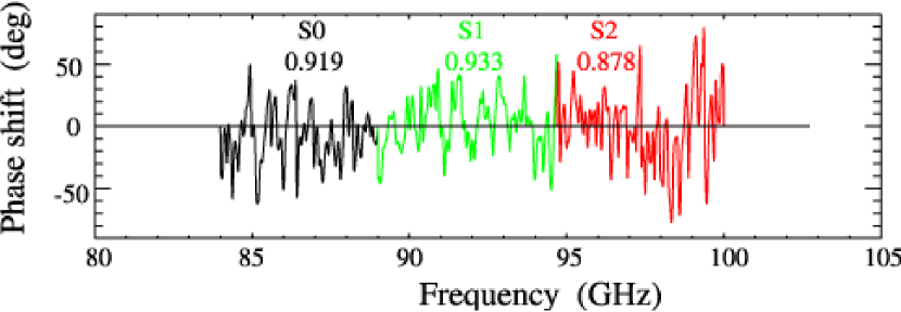
Figure 5: Example of phase-matched phase data from a W-band polarimeter (PIQUE 2001). The three sub-bands are shown in different shades. The numbers printed on the plot are the parameter $\left\langle\cos\phi\right\rangle$ for each band. Some of the oscillatory features are due to standing waves between the injector and the polarimeter, and do not correspond to real phase differences.

By adjusting the phase trimmers in the IF section and inserting shims in the relevant parts of the polarimeter, the phase shift can be adjusted to be near zero across the entire band of interest. Figure 5 shows typical phase data from a phase-matched polarimeter. The phase averages around zero, with variations of $\pm 30^{\circ}$. These variations in $\phi(\nu)$ degrade the effective sensitivity by a factor $\int{g(\nu)\cos\phi(\nu)\,d\nu}/\int{g(\nu)\,d\nu}$, i.e. the gain-weighted average of $\cos\phi$. In practice, we use the unweighted band average, $\left\langle\cos\phi\right\rangle=\int\cos\phi(\nu)\,d\nu/\int d\nu$, as an estimate of how $\phi$ affects the sensitivity of the polarimeter. This parameter is within a few percent of the weighted average and is simpler to measure because it is insenstive to any frequency-dependent variations in the source intensity.

Typically, the average phase shift is measured multiple times with different combinations of shims in the LO lines and with the phase tuners in different positions until the parameter $\left\langle\cos\phi\right\rangle$ is maximized. The final values of this parameter are shown in Table 7 and range from 0.73 to 0.94 with a median value of 0.87. The sensitivity of the polarimeters is degraded by only about 15% due to these residual phase shifts (see § 7.2.2).

4.3.2 Polarized Gain Calibration

The responsivity of the polarimeters is also calibrated prior to their installation on the telescope. The total power channels are calibrated during the Y-factor tests described above, but the polarimetry channels can only be calibrated using specialized sources. These sources must produce broadband thermal radiation with a small polarized component ($U<1$ K). The size of the polarized component must also be calculable from first principles.

In PIQUE, the primary laboratory calibration source consisted of two thermally regulated rectangular waveguide loads. Each load produced thermal radiation polarized along one of two orthogonal axes, which was coupled into the polarimeter through an OMT rotated by $45^{\circ}$ with respect to the polarimeter’s natural coordinate system. The input polarized signal was simply one-half the temperature difference between the loads, and the polarimeter could be calibrated by setting the temperatures of these loads to a variety of values. While this calibration technique was successful for both PIQUE and CAPMAP polarimeters, it required replacing the horn and lens with a system of waveguide, and it could take up to a day to calibrate a single radiometer due to the load’s thermal time constant.

For CAPMAP, a novel calibration method using beam-filling emissive metal plates was developed, which can be performed quickly on fully assembled polarimeters with feed systems installed. Both the thermal emission and the reflected radiation from a metal plate are weakly polarized due to the finite conductivity of the material (see for example Staggs et al. (2002); Cortiglioni (1994); Strozzi & McDonald (2000)). The orientation of the polarized signal is parallel to the plane of incidence, and the received signal is given by

$$P=\sqrt{4\pi\epsilon_{o}\nu\rho}\left(\sec\theta-\cos\theta\right)\left(T_{plate}-T_{load}\right),$$ (12)

where $\rho$ is the resistivity of the metal (in SI units), $\nu$ is the band center frequency, $\theta$ is the angle of incidence, $T_{plate}$ is the physical temperature of the plate, and $T_{load}$ is the temperature of the radiation reflecting off the plate. For an instrument viewing a liquid nitrogen temperature load through a room temperature aluminum plate tilted at $45^{\circ}$, the polarized signal is roughly $100$ mK. Note that the total thermal load on the polarimeter is comparable to the load when the polarimeter is viewing the sky.

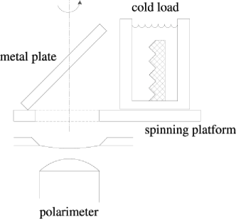
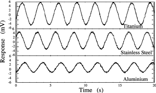
Figure 6: The “miniplate” calibration system used for CAPMAP. (a) Radiation from a cryogenic load reflects off a metal plate into the polarimeter. The figure is a cut through the plane of incidence. Upon reflection and emission from the plate, the radiation acquires a calculable polarized component. Its orientation is parallel to the plane of incidence and its magnitude depends on the composition of the plate and the temperature difference between the plate and the load. By rotating the plate about a vertical axis, the orientation of the polarized signal is modulated. A box of microwave absorber surrounding the system (not shown) prevents stray radiation from contaminating the measurement. (b) Example of data from the miniplate calibration system. The three panels show time series from a single polarimetry channel with three different metal plates: grade 5 titanium, stainless steel 305, and aluminum 6061. Note that metals with higher resistivity produce a larger signal. See § 4.3.2 for a more in-depth description.

This kind of calibration method was used in both CAPMAP and PIQUE to provide an absolute calibration while the instrument was deployed at the telescope, using a large metal plate that nutated over a small range of angles (see § 7.2.1), with the atmospheric emission observed at constant elevation providing the incoming signal. After the first season of CAPMAP, a variation on this technique was developed which could be implemented in the lab. This “miniplate” system consists of a small metal plate that reflects radiation from a liquid nitrogen temperature load into the polarimeter (see Figure 6). The plate and load sit on a mount that rotates about the vertical axis of the polarimeter. The rotation sinusoidally modulates the polarized signal, isolating it from any offsets. Different plates with different resistivities provide consistency checks on the calibration.

Figure 6 shows data taken using three different plates with different resistivities (grade 5 titanium, stainless steel 305, and aluminum 6061, with resistivities of 176, 72, and 4 $\mu\Omega\cdot$cm respectively). These data show that the signal size increases with increasing resistivity as expected. Care must be taken in the design of the system to minimize spurious polarized signals from the room or from the edges of the mount and plate; having data from multiple plates allows any residual contamination from these sources to be identified and removed. The resulting responsivity estimates are consistent with data from the operational telescope (see § 7.2.1).

Limited Dynamic Range of Multipliers

The responsivity measurements not only calibrate the polarimeter, but also insure that it is operating within the limited dynamic range of the multipliers. The double balanced mixers used as multipliers in PIQUE and CAPMAP, like all analog multipliers, are composed of diodes (Pozar, 1998) that operate linearly only over a limited range of input powers. If the input power is too high, the multiplier output is compressed, and if it is too low, the Johnson noise of the multiplier contributes significantly to the output rms fluctuations.

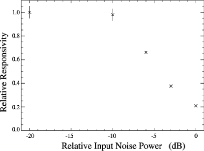
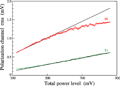
Figure 7: Gain compression of the multipliers with increased total power loading. (a) Data showing that the relative responsivity (the multiplier’s response coefficient) decreases monotonically for large total power input. The errors for the large input powers are smaller than the size of the point. Data come from PIQUE lab tests. (b) The rms of the multiplier output versus a variable total power input. The straight line is fit to the lower half of the data for the top curve (S0), and to the upper half of the data for the bottom curve (S1). S0 shows saturation while S1 shows the onset of Johnson noise domination. Data come from CAPMAP lab tests. Refer to § 4.3.2 for more details.

Compression at high input power levels occurs due to the diodes’ nonlinear I-V curve. The nonlinear behavior of diodes allows them to operate as multipliers to first order in the input fields. However, if the input power is too high, additional nonlinear terms couple the responsivity of the multiplier to the total input power on the polarimeter (see Figure 7). In this regime, the responsivity of the instrument to polarized signals decreases monotonically with increasing system temperature. Only if the total power reaching the multiplier is kept below roughly 10 $\mu$W will the polarimetry channel responsivity be independent of loading.

By contrast, if the total power reaching the multiplier is too low, the intrinsic Johnson noise of the multiplier will contribute significantly to the rms fluctuations at the output and decrease the sensitivity of the polarimeter. The Johnson noise of the multiplier does not significantly affect the sensitivity as long as the total power at the multiplier is greater than about $1~{}\mu$W. The range of gains where the Johnson noise is not significant and the responsivity of the multiplier is not dependent on the total power is therefore fairly narrow (see Figure 7), and the total power reaching the multipliers must be carefully adjusted with drop-in attenuators prior to fielding the instrument.

5 OPTICS

Both PIQUE and CAPMAP use off-axis telescopes, which have no central blockage and little scattered radiation from the support structures. However, off-axis optical elements also produce a nonzero polarized signal oriented along the plane of symmetry. The polarimeters in both experiments are thus oriented so that they are largely insensitive to this sort of signal—they measure $U$ instead of $Q$ in the telescope’s coordinate system.

The optics of the two experiments are very different. PIQUE used a 1-meter mirror that was easily installed in a temporary rooftop observatory and was small enough to be contained in a full-sized set of ground screens. CAPMAP uses a 7-meter telescope, which is too large to be fully enclosed in ground screens, but which can provide higher angular resolution and a larger focal plane. PIQUE and CAPMAP are discussed separately below.

5.1 PIQUE Optics

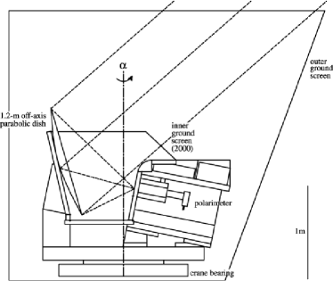
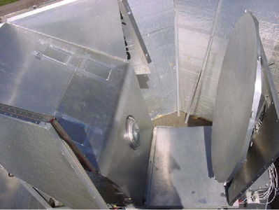
Figure 8: PIQUE optics. (a) A corrugated feed horn on the polarimeter views a 1.2 m off-axis parabolic mirror. A crane bearing in the base of the telescope allows it to slew in azimuth, $\alpha$, at a fixed elevation. Two nested ground screens block radiation from local sources. The outer ground screen is fixed to the ground while the inner ground screen rotates with the base. The inner ground screen here was used during the first observing season. During the second observing season this ground screen was made twice as tall. (b) Photo of the PIQUE telescope taken from the top of the outer ground screen. The side panels of the inner ground screen have been removed for the photo.

The PIQUE polarimeter viewed the sky through a corrugated feed horn and an off-axis parabolic mirror. The entire telescope was mounted on a crane bearing so the antenna could scan in azimuth at a fixed elevation of about $41^{\circ}$ (see Figure 8).

5.1.1 Optical Components

The parabolic mirror was originally built for the Saskatoon experiment and is described in detail in Wollack et al. (1997). It has a focal length of 75 cm and an effective diameter of 122 cm, and the optical axis is offset 78 cm from the center of the mirror. The rms roughness of the surface is better than 50 $\micron$.

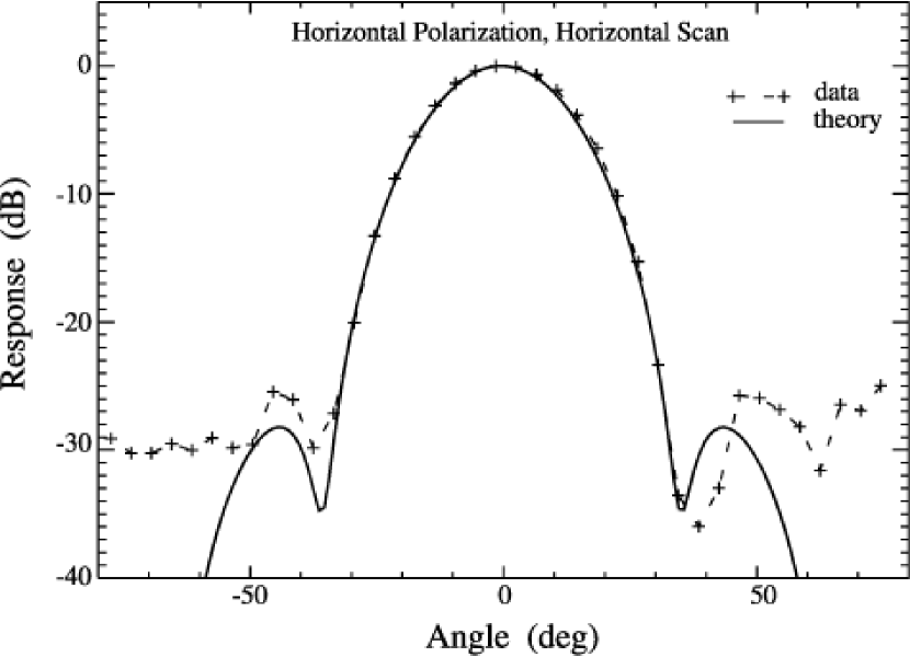
Figure 9: The predicted (solid) and measured (dashed) beam patterns of the PIQUE W-band horn. The $-30$ dB level is the noise floor of the experimental apparatus used here.

The W-band horn was specially made for PIQUE. This horn was designed using the physical optics program CCORHRN (James, 1981) to illuminate the mirror with an edge taper of $-25$ dB. This criterion determined the length and aperture diameter of the horn, given in Table 8. To achieve acceptable polarization fidelity, the horn was corrugated with grooves whose depth and width were the same as for the WMAP feeds (Barnes et al., 2002), and the throat section had progressively deeper and narrower grooves following the prescription in Zhang (1993). The horn was made from electroformed copper plated in gold. Its measured beam size was $25^{\circ}$ with side-lobe levels below $-25$ dB, closely matching the theoretical predictions (see Figure 9).

The expected telescope FWHM was $0.25^{\circ}$ at 90 GHz and $0.50^{\circ}$ at 40 GHz. The exact placement of the polarimeters was determined using observations of a near-field source of narrow-band radiation. The response of the telescope as a function of elevation and azimuth uniquely determines the location of the polarimeter relative to the mirror, and by comparing the observed data to the predictions from the physical optics program DADRA (Imbriale & Hodges, 1991; Imbriale, 2003), it was possible to locate the horn to within 3 mm of the focal point. Observations of Jupiter, discussed in § 7.1.1, confirm that the telescope was aligned properly.

5.1.2 Ground Screens

The PIQUE telescope was located on the roof of Jadwin Hall in Princeton, New Jersey. Two nested ground screens were installed around the telescope to prevent stray radiation generated by surrounding buildings from reaching the telescope (see Figure 8). The outer ground screen was fixed to the roof and geometrically blocked all radiation from external sources. It had the shape of an inverted, truncated hexagonal pyramid with a 3.3 m footprint, a height of 3.3 m, a vertical southern wall, and five other walls sloping outward at $20^{\circ}$. The interior walls of this ground screen were lined with aluminum-covered styrofoam, and each panel was hinged at its mid-height so the entire structure could be covered in case of bad weather.

The inner ground screen, which was made of aluminum, was attached to the telescope base and rotated with the telescope. In its initial configuration, it blocked all radiation emanating from the edge of the outer ground screen and above; radiation from the outer ground screen itself could reach the polarimeter, producing an azimuth-dependent polarized offset of a few hundred $\mu$K (see § 8.3). To reduce these offsets, the inner ground screen was enlarged for the second observing season to block the outer ground screen as well; the results of this improvement are discussed in § 8.3.

5.2 CAPMAP Optics

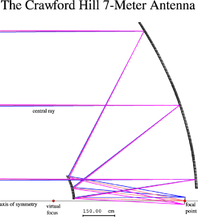
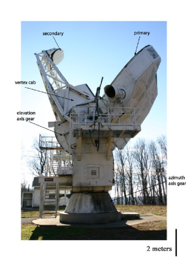
Figure 10: CAPMAP optics. (a) Side view scale drawing of the 7-meter telescope pointing at an elevation of $0^{\circ}$. Three bundles of rays are drawn from the Cassegrain focus to the secondary with an illumination half angle of $5^{\circ}$. (b) Photograph of the off-axis Cassegrain 7-meter telescope. The radiation is focused onto the feed horns in the focal plane. The receivers are enclosed in the vertex cabin around the focal point.

CAPMAP uses the Crawford Hill 7-meter antenna located in Holmdel, NJ. A comprehensive description of the antenna is given in Chu et al. (1978), and its optical parameters are summarized in Table 8. It is an off-axis Cassegrain telescope with a 7-meter primary and a 1.2 m $\times$ 1.8 m oval secondary, oversized in the horizontal direction (see Figure 10). The primary reflector is made of 27 aluminum panels arranged in 4 concentric rings. The surface accuracy of each panel is $\sim 50$ $\micron$, and the surface error of the overall primary reflector is 100 $\micron$ rms. The telescope is mounted on a standard alt-az platform with two DC motors on each axis, allowing a maximum slew speed of 2 deg$\cdot$s^-1 in azimuth and 1 deg$\cdot$s^-1 in elevation. The telescope features a remarkably large and high-quality focal plane with Strehl ratios above 0.97 up to 0.5 m from the focal point, making it possible to field an array of receivers while maintaining excellent beam quality. The telescope also has a cross-polarization response in the main beam below $-40$ dB (Chu et al., 1978).

The large 7-meter primary mirror produces a beam narrow enough to resolve the anisotropy of the CMB polarization, but it also precludes the feasible construction of a PIQUE-style ground screen. We therefore sacrifice resolution and aggressively under-illuminate the primary and secondary at approximately $-35$ dB and $-58$ dB to reduce spillover and produce a $0.065^{\circ}$ (4’) FWHM beam at W-band and a $0.10^{\circ}$ (6’) beam at Q-band. This requires a narrow, $2.3^{\circ}$ beam from the feed system with minimal sensitivity outside the edge of the secondary ($5^{\circ}$ half angle). The feed system must also be compact for practical cryogenic cooling.

5.2.1 Feed System

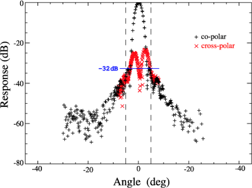
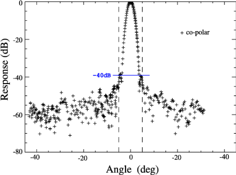
Figure 11: Co- and cross-polar beam maps of CAPMAP feed systems during the 2003 (left) and 2004 (right) observing seasons. The measurements were made from the testing range on the roof of Jadwin Hall, where beams can be mapped down to the $\sim-50$ dB noise level. Co-polar maps are shown with plus symbols and cross-polar maps with crosses. The vertical dashed lines at $\pm 5^{\circ}$ show the illumination at the edge of the secondary mirror. During the first season, the edge taper on the primary was $-32$ dB with a cross-polar maximum at $-25$ dB. The lenses were redesigned for the second season to achieve an edge-taper of $-40$ dB and a cross-polar level $<-40$ dB. (The cross-polar level was too small to be determined reliably from this measurement; it has been inferred from the quadrupole leakage as explained in § 8.2.)

To satisfy these criteria, the CAPMAP feed system consists of a compact profiled horn coupled to a lens. The design of the CAPMAP horn is similar to that used in PIQUE, except that the profile is optimized to reduce the side-lobes from the horn and to improve the Gaussianity of the beam. The CAPMAP optical system is detailed in McMahon (2005). The horn produces a $14.5^{\circ}$ beam that deviates from a Gaussian at the $-35$ dB level. The beam propagates through free space to a high-density polyethylene (HDPE) lens which re-converges the beam. The focal length and diameter of the lens were chosen to minimize the amplitude of the side-lobes while maintaining a $2.3^{\circ}$ beam. This process produces a first side-lobe at $-40$ dB below the peak of the main beam, which is Gaussian down to that level (see Figure 11).

For the first observing season, the lenses had spherical rear and elliptical front surfaces. In such a lens, refraction only takes place at the front surface, where the angle of incidence is as high as $60^{\circ}$. For normal incidence along $\hat{z}$, the transmission coefficients of the two orthogonal field components $E_{x}$ and $E_{y}$ are the same, but the two coefficients deviate as the angle of incidence increases, since boundary conditions differ for field components perpendicular and parallel to the interface. The difference between the two transmission coefficients was increased in CAPMAP 2003 by the lens anti-reflection (AR) coating, which consisted of concentric near-quarter-wave grooves on the lens surfaces. Since these grooves are not locally symmetric under $90^{\circ}$ rotations, they have different refractive indices for the two orthogonal polarizations. These effects produce cross-polarization, in which polarized sources viewed off the beam center couple to the orthogonal polarization inside the horn throat. This causes unpolarized point sources viewed off the beam center to produce a spurious polarized response with a quadrupolar symmetry; the implications for the performance of the experiment are discussed in § 8.2.

For the 2003 season, the level of cross-polarization was $-24$ dB. For the 2004 season, the lenses were re-designed to share the refraction evenly between the front and back surfaces, reducing the maximum angle of incidence to $30^{\circ}$ on both surfaces. In addition, the AR coating was changed to a square array of holes, which—being locally invariant under $90^{\circ}$ rotations—has equal transmission coefficients for each linear polarization. These modifications significantly improved the cross-polarization of the lenses, which was reduced below $-40$ dB (see § 8.2).

5.2.2 Focal Plane

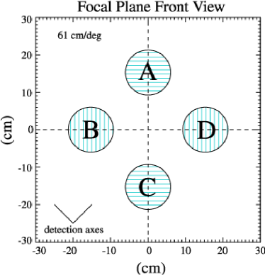
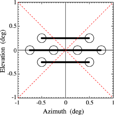
Figure 12: (a) Focal plane layout in the CAPMAP 2003 dewar as seen from the secondary. The cross-hatch indicates the direction of the E-plane polarization of the main arm of the OMT. The resulting detection axes are at $45^{\circ}$ from the OMT axes. Each circle represents the position of the lens. The receivers are tilted $1.7^{\circ}$ inwards in the focal plane to point towards the center of the secondary. The position of the beams on the sky with respect to the center of the array is reversed in both the up-down and left-right orientation. As seen from the focal point, the arrangement of the beams on the sky has A on the bottom, B on the left, C on the top, and D on the right. (b) CAPMAP 2003 azimuth scan pattern on the sky. Each horn is designated by a circle. The NCP is at the origin. A horn on the thin solid lines measures U alone, and a horn on the dashed lines measures Q alone; otherwise each horn measures a combination of Q and U.

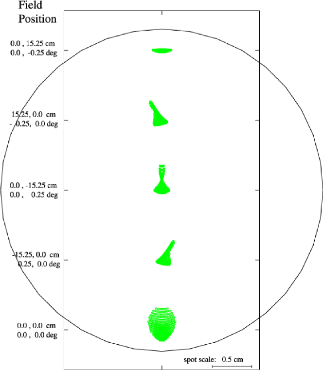
Figure 13: Spot diagrams of the Crawford Hill antenna. The spot diagrams are calculated using the CODE V software. The five spots displayed are the dispersion of $\sim 300$ rays distributed over the whole primary and focused to the focal point and the four CAPMAP 2003 horn positions. The large circle is the diffraction beam size of the fully illuminated telescope for the focal point spot (scaled by the plate scale). These data agree with the fact that the beam distortions are very small away from the focal point. The Strehl ratios for the four beam positions are better than 0.99.

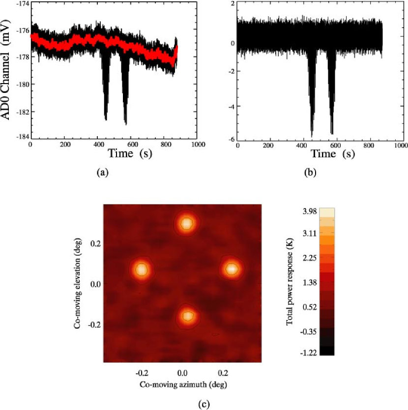
Figure 14: Illustration of the Jupiter and radio sources data processing. (a) Time series of one total power channel during an observation of Jupiter (black), with the baseline fit (red) overlayed. Note that each of the two bumps represents approximately 20 source rasters at different elevations; the $x$ axis is too large to resolve each individual Gaussian. (b) The same time stream with the baseline drift removed. The baseline fit removal is equivalent to a pre-whitening filter and is only applied to the total power channels. (c) Mosaic map of the CAPMAP 2003 focal plane from a single 15-minute Jupiter observation taken on 2003 February 12, using the time series processing described above. The angular diameter of Jupiter was 45$\arcsec$ on this date. The black contours correspond to power levels of 10% and 50% of the peak value.

The CAPMAP 2003 focal plane layout consists of four receivers located 15.25 cm on either side of the focal point arranged in a diamond pattern as in Figure 12. Given the 68.9 cm$\cdot$deg^-1 plate scale, the four horns are spaced $0.25^{\circ}$ equidistant from the central ray on the sky. Although the receivers are packed relatively tightly to keep the scan region compact, they are not packed as tightly as possible to the focal point because the 7-meter antenna provides a large focal plane with undistorted beams out to 40 cm away from the focal point. This fact was first simulated with ray tracing (Figure 13) and physical optics software; it was confirmed by beam maps of the receivers on Jupiter, shown in Figure 14. In order to minimize the induced polarization from the telescope mirrors, each receiver is tilted $1.7^{\circ}$ to point towards the center of the secondary. This geometric arrangement of the horns also satisfies the azimuth scan strategy suggested by Wollack et al. (1997), which was used for the first observing season.

The azimuth scan swept the telescope in azimuth across the NCP at constant elevation with an 8 second period. The constant elevation avoids the $\sec\theta$ total power modulation from the atmosphere. Figure 12 shows the path traced out by the four horns in a single scan across the NCP. The scan amplitude of $\sim 0.5^{\circ}$ was chosen to optimize the signal-to-noise ratio per pixel given the sensitivity of the array.

Since the Crawford Hill telescope has a large $f/D$ ratio (it is a slow optical system), the tolerance on the position of the receivers in the focal plane is quite large. Mechanical alignment methods were therefore sufficient to position and orient the polarimeters on the telescope for the first observing season. For the subsequent observing season, the goal for accuracy in the relative alignment of the receivers was $0.4\arcmin$, or a tenth of a W-band beam size. This goal corresponds to the requirement that the dewars be positioned with an accuracy of 4 mm. Observations of Jupiter were used to verify this alignment.

6 SITE ATMOSPHERIC CONDITIONS

Both PIQUE and CAPMAP are based in central New Jersey. Although New Jersey is not considered a prime location for millimeter wave observation, we have evidence that the atmospheric conditions are sufficiently good for E-mode polarization measurements at 90 GHz. Primarily, three factors affect the quality of observations: cloud coverage, atmospheric temperature, and atmospheric water content. Table 9 lists observed characteristics for the 2003–2004 winter.

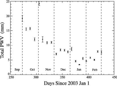
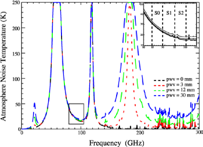
Figure 15: Crawford Hill atmospheric environment. (a) Time series of the total PWV during the winter 2004 observing season, rebinned in 10-day intervals. These data are derived from the hourly GOES satellite archives. The precipitable water vapor (PWV) is the average from a 100 km square grid centered on Crawford Hill. The 50% quartiles for the months of October through February are 12.8, 12.8, 7.0, 4.0, and 4.8 mm respectively. (b) Atmospheric zenith emission temperature versus frequency for different values of PWV. Inset is a zoom on the three CAPMAP frequency bands. The three values of PWV (3 mm, 12 mm, and 30 mm) are representative of the best, average, and worst observing conditions respectively. The line shapes were generated using E. Grossman AT software (1989), with the following parameters: full Lorentzian line profile, elevation = 100 m, latitude = $40^{\circ}$, zenith angle = $0^{\circ}$, physical temperature of the atmosphere = 250 K. The AT software produces the atmospheric transmission, $t$, which was converted into a zenith sky temperature as $T_{atm}=250(1-t)$.

At 90 GHz, apart from very high and thin cirrus clouds, any cloud coverage prevents all observations. Table 9 shows that December, January, and February are the clearest months, with a perfectly clear sky nearly 40% of the time. The atmosphere at 90 GHz has a finite opacity, which is dominated by the wings of the emission lines from molecular oxygen and water vapor (see Figure 15). The emission from oxygen sets a lower limit on the atmospheric noise temperature at the site, but the more variable water vapor content provides a better measure of the data quality.

The precipitable water vapor (PWV)—the total height of liquid water condensible from a column of atmosphere—is therefore often used as a standard figure of merit to compare different millimeter wave observing sites. Figure 15 shows the time series of the PWV in Crawford Hill during the 2003–2004 winter. The three months of December, January, and February consistently have the lowest PWV and the best data quality. PWV values as low as 1.6 mm were recorded and lasted for periods of 10 to 24 hours.

7 ON-SITE PERFORMANCE

The PIQUE and CAPMAP instruments together have taken data during four of the last five winters. The PIQUE telescope first came online on the roof of Jadwin Hall on 2000 January 1 and operated until 2000 May 8, at which time the polarimeter was brought to the lab for the summer. The instrument was installed the next winter on 2000 December 15 and operated until 2001 February 28, at which point the W-band polarimeter was removed, and the Q-band system took data until 2001 May 10. The CAPMAP 2003 instrument, consisting of four W-band polarimeters, was brought to the 7-meter telescope on 2003 January 16. The CMB observing season lasted from February 18 to April 6. The instrument remained on the telescope until 2003 June 18 for various post-season investigations. In the 2003–2004 winter, 9 W-band and 3 Q-band polarimeters operated intermittently at the Crawford Hill telescope, and the full 16-element array was installed for 2004–2005.

Thus far, only data from the PIQUE W-band system and the first CAPMAP observing season have been fully processed and analyzed. A breakdown of the time spent on various activities for the various observing seasons is given in Table 10. Most of the available time is dedicated to observations of the CMB near the NCP, which are described more thoroughly in Hedman et al. (2001, 2002) and Barkats et al. (2004). Additional data from astronomical and local sources needed to calibrate the operational telescopes are described in the next two sections.

7.1 Total Power Channel Performance

The total power channels quantify the receiver noise temperatures and the opacity of the atmosphere during the CMB observing seasons, so we calibrate the total power channels using observations of Jupiter and elevation scans through the atmosphere. These data also provide estimates of the beam size, pointing solution, and noise temperature of each telescope.

7.1.1 Jupiter Observations

Jupiter is a bright, compact, unpolarized source at millimeter wavelengths (de Pater, 1999), so observations of this planet are used to calibrate the total power channels and to measure the beam size and pointing of the operational telescope. These observations also provide important information about the polarization-specific systematic effects discussed in § 8.

PIQUE and CAPMAP have observed Jupiter in slightly different ways. The PIQUE telescope cannot scan in elevation, so Jupiter observations consisted of repeated scans in azimuth lasting for a period of about 10 minutes, during which time Jupiter passed through the observed elevation. By contrast, the CAPMAP telescope scans back and forth in azimuth over a specified range of about $1^{\circ}$ and then steps in elevation by about $0.02^{\circ}$. Repeating this pattern of movements covers a two-dimensional area centered on the nominal position of Jupiter.

For any of these observations, the data from each total power channel is processed to produce a two-dimensional beam map. Figure 14 illustrates the analysis process. First, any drifts in the time series are removed using a baseline fit generated from the data taken when the telescope was pointed at blank sky to the left or right of Jupiter. After subtraction of this baseline fit (which effectively pre-whitens the data), the data are binned in coordinates centered on the nominal position of Jupiter, producing a two-dimensional map of the telescope response.

Not all observations of Jupiter produced useful maps. Clouds or other atmospheric phenomena passing through the scan region corrupted some observations so that it was not possible to extract a clean map of the signal from Jupiter. These observations are easily identified and removed, leaving 12 successful observations for each season of PIQUE and 15 observations for the first season of CAPMAP.

For each successful observation, the map for each channel is fit to a two-dimensional Gaussian:

$$f(x,y)=A\exp\left\{-\frac{(x-x_{0})^{2}}{2\sigma_{x}^{2}}-\frac{(y-y_{0})^{2}}{2\sigma_{y}^{2}}\right\},$$ (13)

where $x$ and $y$ are the cross- and co-elevation of the telescope relative to Jupiter, and $A$, $x_{0}$, $y_{0}$, $\sigma_{x}$, and $\sigma_{y}$ are fit parameters.

The Gaussian beam widths $\sigma_{x}$ and $\sigma_{y}$ for all the observations with either telescope have a scatter consistent with their errors determined by the fitting algorithm. There is no evidence that different total power channels or different polarimeters of the same band have significantly different beam sizes, so all of these data are averaged together to obtain the final estimates of the telescope beam shape (see Table 11). The uncertainties in these estimates are derived from the scatter of the individual estimates and do not significantly affect the analysis of the CMB data (Barkats et al., 2004). Furthermore, the measured beam widths are consistent with the predictions based on physical optics programs, and there is no significant ellipticity; the evidence indicates that both telescopes were well focused.

The offset parameters $x_{0}$ and $y_{0}$ establish the telescope pointing. For PIQUE the pointing solution was not well constrained, because Jupiter could only be observed in two positions as it rose or set through the elevation range visible to the telescope. The measured pointing offsets at these two locations were not consistent with each other and indicate some azimuth-dependent offset term that must be extrapolated to the NCP. This extrapolation increases the uncertainty in the pointing error to approximately $0.1^{\circ}$, which did not significantly affect our limit on the CMB polarization (Hedman et al., 2001). For CAPMAP, Jupiter and other radio sources—Cas A, Tau A, Orion (OMC-1), and Cyg A—were observed at a high signal-to-noise ratio at a wide variety of positions. These data strongly constrain a pointing model and reduce the rms uncertainty in the telescope pointing near the NCP to less than $30\arcsec$.

Lastly, the parameter $A$ serves to calibrate the total power channels, given an estimate of the peak signal from Jupiter

$$t_{jup}=\tau_{atm}T_{jup}\Omega_{jup}/\Omega_{tel}.$$ (14)

The effective temperature of Jupiter at 90 GHz $T_{jup}=171$ K is based on WMAP data (Page et al., 2003). The solid angle subtended by Jupiter’s disk $\Omega_{jup}$ is computed from ephemeris data. The beam solid angle $\Omega_{tel}=2\pi\sigma_{x}\sigma_{y}$ is calculated from the beam widths measured above. The atmospheric transmission coefficient $\tau_{atm}$ is derived directly from the total power level for the blank sky during the observation.

The responsivity estimates derived from Jupiter observations are consistent with estimates derived from the Y-factor tests described in § 4.3.1. For PIQUE, the two sets of estimates agree to within 15%, while for CAPMAP they agree to better than 10%. The residual discrepancies between the two methods are statistically significant—the Jupiter estimates are consistently lower than the Y-factor estimates—which implies the optical systems have a finite loss of roughly 6%. This estimate is consistent with the data from elevation scans in CAPMAP (see § 7.1.2). Even if the discrepancy is due to an unknown systematic effect in one of the two methods, a 10%–20% calibration error in the total power channels does not significantly affect the analysis of the CMB data.

7.1.2 Atmospheric Elevation Scans

Atmospheric elevation scans are performed by scanning the telescope in elevation between the horizon and the zenith at a fixed azimuth. These observations of the atmosphere, which can only be done with the CAPMAP telescope, provide an estimate of the noise temperature of the entire telescope (including the optics), unlike the Y-factor tests described previously, which only measure the noise temperature of the polarimeter itself.

The receiver noise temperature on the telescope ${\widetilde{T}_{rec}}$ remains constant as the telescope scans, while the atmospheric noise temperature varies as $T_{z}\csc(el)$, where $el$ is the telescope elevation and $T_{z}$ is the atmospheric noise temperature at zenith. The total system temperature, neglecting the CMB contribution, as a function of elevation is therefore $T_{sys}(el)={\widetilde{T}_{rec}}+T_{z}\csc(el)$. The total power channels, with gains calibrated using the Jupiter observations, provide estimates of $T_{sys}(el)$, which are then fit to the appropriate functional form to obtain estimates of ${\widetilde{T}_{rec}}$ and $T_{z}$.

Ideally, the estimates of ${\widetilde{T}_{rec}}$ and $T_{z}$ from different scans should be uncorrelated. However, during the first observing season there was a significant correlation between the estimated receiver noise and $T_{z}$. This correlation occurred because side-lobes behind the primary mirror (discussed in § 8.3) alter the shape of the $T_{sys}(el)$ curve. The available data are insufficient to model this effect precisely, so we estimate ${\widetilde{T}_{rec}}$ simply by extrapolating to the value with $T_{z}=0$.

The final estimates of the telescope noise temperatures are given in Table 6, which shows that the telescope noise temperatures for polarimeters $A$ and $C$ are much higher than the noise temperatures of the other polarimeters. (This excess noise was also observed with Y-factor tests at the telescope.) This excess noise is inconsistent with the polarimetry channel sensitivities (see § 7.2.2), and is an artifact caused by the IF amplifiers used in these polarimeters. While these amplifiers performed well individually, when they were all installed together in a single box, they produced significant noise at frequencies below 2 GHz, which can be detected by the unfiltered total power channels but is outside the polarimetry bands. Polarimeters $B$ and $D$ used amplifiers with smaller gain and better power regulation and did not have this problem. After the first observing season the amplifiers in polarimeters $A$ and $C$ were replaced, and excess noise in the total power channels was no longer observed. This out-of-band noise also did not affect the quality of the polarimetry data from the first observing season in any detectable way.

For polarimeters $B$ and $D$ in 2003, Table 6 shows that ${\widetilde{T}_{rec}}-T_{rec}\approx 15$ K, implying that the full optical path at the telescope has a loss of roughly 6%. This loss can arise from both absorption through the windows and diffuse scattering from the mirrors in the optical path; it is consistent with the material properties of these objects.

7.2 Polarimetry Channel Performance

Astronomical and local sources of polarized radiation serve to calibrate the polarimetry channels, while observations of the atmosphere quantify the sensitivity of the polarimeter. These observations are also used to derive the polarization-specific systematic effects described in § 8.

7.2.1 Calibration

We have already discussed in § 4.3.2 several methods of calibrating the responsivity of the polarimetry channels in the laboratory. Two additional techniques are used to calibrate the polarimetry data during the observing season: (1) a system based on an emissive chopper plate, and (2) observations of the polarized source Tau A (for CAPMAP only).

The chopper plate calibration system works on the same principle as the miniplate system described in § 4.3.2: the reflection and emission of thermal radiation from a metal surface produce a controlled, calculable broad-band polarized signal. In this case the surface is an aluminum flat 1 meter across by 2 meters tall that nutates sinusoidally about a vertical axis with a period of $\sim 2$ seconds to modulate the polarized signal. This plate reflects thermal radiation from the sky at constant elevation into the polarimeters. For PIQUE, the plate was sufficiently large that it could be viewed by the primary mirror. For CAPMAP, the plate is installed in front of the secondary so that radiation from the sky is reflected directly into the polarimeters.

The geometry of the chopper plate is slightly more complicated than that of the miniplate system because the plate does not rotate about the axis of the feed, but the polarized signal is still given by Equation 12. In this case the atmosphere is the load of the system, and we use the total power channels to estimate $T_{load}$. Statistical uncertainties derived from this method are small, and the systematic uncertainty in the calibration is about 10%, dominated by uncertainty in the resistivity of the aluminum plate. The emissivity of the metal is the same for all polarimeters, so the relative values of the responsivities for different polarimeters are better constrained. Based on the repeatability of this test, the uncertainties in the relative gains of different channels are only a few percent.

Additional calibration data for CAPMAP 2003 are provided by 10 observations of Tau A, a strong source of polarized radiation at 90 GHz. Tau A is sufficiently compact that it can be treated as a point source, and its main polarized component has a well measured position angle of $155^{\circ}$ (Mayer & Hollinger, 1968). Unfortunately, WMAP has not yet provided an accurate estimate of the polarization fraction of Tau A, and the published data have a relatively large scatter of 7.5%$\pm$1.0% (Farese et al., 2004). Thus observations of Tau A cannot provide a precise calibration, but they serve as a useful check on the responsivity estimates from the chopper plate.

The Tau A observations are performed and processed like the Jupiter data to obtain maps of the polarimetry response fit to two-dimensional Gaussians. If the parallactic angle of the polarimeter during the observation is more than $23^{\circ}$ from $155^{\circ}$, then the point polarized source approximation of Tau A breaks down and the observation does not provide useful calibration data. The beam widths derived from the successful fits are significantly different for the different frequency bands, as expected for diffraction-limited optics (see Table 11). These variations in beam size are accounted for in the responsivity calculations in the data analysis.

The responsivity estimates from Tau A are not systematically different from the estimates derived from chopper plate data, and the differences between the two estimates are in general less than 20%.

Gain Variations

The chopper plate and Tau A calibration data also quantify variations in the responsivity of the polarimetry channels due to changes in the temperature of various components. For PIQUE, the dewar was intentionally heated and cooled during one long chopper plate run near the end of each observing season. These data show that the responsivities of the polarimetry channels change by a fraction of a percent for every Kelvin change in the dewar temperature. These variations were sufficiently minor that they could be ignored in the data analysis.

For the first season of CAPMAP, the temperatures of the IF box and the LO varied by roughly 10 K over the course of the season. Tau A data taken with the IF box and LO at different temperatures quantify the effects of these temperature shifts on the responsivity of the polarimetry channels. The polarimetry channels are insensitive to the temperature of the LO, but a 10 K shift in the temperature of the IF box changes the polarimetry channel gain by roughly 10%–20%. This change is consistent with the temperature coefficient of the IF amplifiers and must be accounted for in the processing of the CMB data (Barkats et al., 2004).

7.2.2 Sensitivity

Section 4.3 describes the procedures used to optimize the polarimeter performance. Here we compare the sensitivities achieved with those extrapolated from the characterization. Using typical values for $T_{sys}$ from Table 6, and values of $\Delta\nu$ which take into account the phase factors given in Table 7, Equation 5 yields $S\approx 115\mbox{ K}/\sqrt{3\mbox{ GHz}}\approx 2\mbox{ mK}\sqrt{\mbox{s}}$ in the Rayleigh-Jeans limit. However, while the system temperatures and the calibration source power levels are sufficiently high that the Rayleigh-Jeans limit applies at 90 GHz, the 3 K CMB signal is not, so the responsivity and the sensitivity must be increased by a factor of 1.2 at 90 GHz (Bennett et al., 2003b). Therefore the sensitivity of a single polarimetry channel to variations in the CMB should be roughly 2.4 mK$\sqrt{\mbox{s}}$, and the total sensitivity of a W-band polarimeter with three polarimetry channels should be 1.4 mK$\sqrt{\mbox{s}}$.

The sensitivities of the polarimetry channels can be measured directly from the fluctuations in the time stream when the polarimeter views the sky (in an area free of known sources) and are tabulated in Table 12. The measured sensitivities are consistent with the calculation from Equation 5, indicating that the instruments suffer no excess noise under observational conditions. Note that the sensitivities of CAPMAP polarimeters $A$ and $C$ are comparable to the others, demonstrating that the high telescope noise temperatures given in Table 6 are artifacts.

8 POLARIZATION-SPECIFIC SYSTEMATIC EFFECTS

To detect the small polarized component of the CMB, a polarimeter must not only have sufficient sensitivity to polarized signals, but it must also be able to extract the polarized signal from largely unpolarized radiation. Work is just now beginning on methods to quantify the systematic effects on the quality of CMB polarization data, which will be extremely important as increasingly sensitive arrays of instruments push forward towards the goal of detecting the B-mode component of the polarization (Gaier et al., 2003; Keating et al., 2003; Church et al., 2003).

Hu et al. (2003, hereafter HHZ) have developed a nomenclature that quantifies polarization-specific systematic effects in terms of leakages among Stokes parameters. The dominant instrumental systematic effect in determining E-modes arises from $I\rightarrow Q$ and $I\rightarrow U$ couplings. Mixing between Q and U can confuse E- and B-modes by rotating the detection axes of the polarimeter, but such effects can be neglected in determining the E-modes because observations of polarized sources—such as the moon and Tau A—show that the detection axes are within $3^{\circ}$ of the expected orientation. Spurious responses of the polarimeter to unpolarized incident radiation may be broadly classified into three types: (1) monopole leakage (often called instrumental polarization, or “polarization transfer” in HHZ) arising from an axially symmetric unpolarized source; (2) leakage from off-axis sources (also called dipole/quadrupole leakage or “local contamination” in HHZ), arising from local curvature of the optics and typically dominated by response to unpolarized dipole and quadrupole source distributions; and (3) polarized far side-lobes.

8.1 Monopole Leakage

We follow the convention in HHZ and quantify the monopole leakage with the parameter $\gamma$, which is the apparent change in the polarized signal per unit change in the unpolarized intensity of the axially symmetric incident radiation. This parameter is proportional to the Mueller matrix element $m_{\rm UI}$ (Heiles et al., 2001). For PIQUE and CAPMAP, this leakage term arises primarily from the limited isolation of the output ports of the OMT, as we describe below.

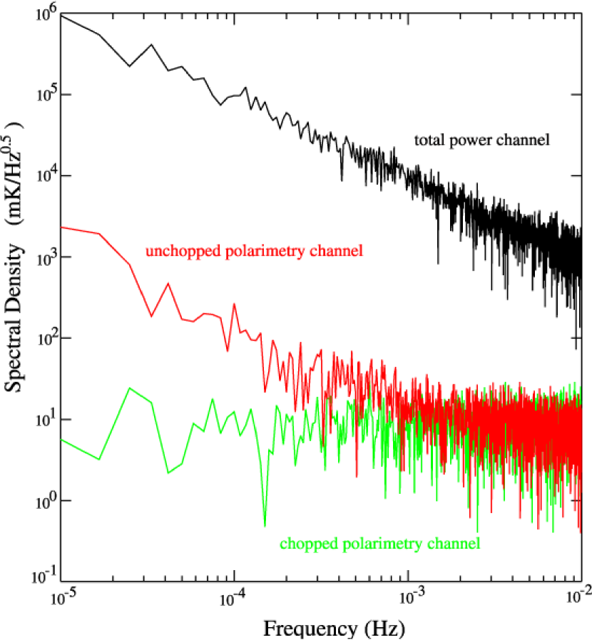
Figure 16: Power spectrum of various PIQUE data channels from a clear day in February 2000 in NJ. The black curve shows the power spectrum of a total power channel, which does not have 4 kHz modulation. The spectrum has a pronounced slope characteristic of $1/f$ noise due to drifts in the temperature of the atmosphere. (The contribution from drifts in the polarimeter is sub-dominant on all time scales displayed here.) The red curve is a polarimetry channel after demodulation at 4 kHz. The $1/f$ noise is much reduced, and becomes sub-dominant to the white thermal noise on time scales less than several minutes. The PIQUE and CAPMAP systems scan over the sky with periods of roughly 8–12 seconds. The signal from the sky is modulated on this time scale and has a purely thermal noise spectrum (green line) for time scales less than a day.

The value of $\gamma$ can in principle be estimated by measuring the response of the polarimetry channels to changes in the temperature of an unpolarized load. However, for small values of $\gamma$, it is difficult to create a load sufficiently unpolarized for a reliable measurement. Observations of the atmosphere at different elevations do appear promising, but the effects of orientation-dependent signals from side-lobes are still under investigation. A more practical method of estimating $\gamma$ is to observe a quiet patch of sky (see Figure 16). The atmosphere is essentially unpolarized (Keating et al., 1998; Hanany & Rosenkranz, 2003), but the temperature of the atmosphere drifts such that the power spectrum of the fluctuations in the total power channels (black line in Figure 16) has a strong $1/f$ component. If $\gamma=0$ and if the atmosphere were completely unpolarized, the power spectrum of the polarimetry channels would have no $1/f$ noise. However, the actual polarimeters have a nonzero $\gamma$, and their power spectra have a $1/f$ component that dominates on time scales longer than 1000 seconds (the red curve in Figure 16). The ratio of the levels of the $1/f$ components in the total power and polarimetry channels provides a good estimate of $\gamma$, which is roughly $-23$ dB for both the PIQUE and CAPMAP polarimeters.

For correlation polarimeters, a nonzero $\gamma$ occurs because some radiation in one arm of the polarimeter leaks into the other arm before the phase switch and generates a nonzero output voltage from the multiplier. Because this signal is modulated by the phase switch like a real polarized signal, it is not eliminated by the demodulation process. In PIQUE and CAPMAP, the measured value of $\gamma$ is consistent with leakage through the OMT. A real OMT couples a small fraction of each polarized component into the wrong arm of the polarimeter. This “direct” leakage between the arms does not produce a significant $\gamma$ term because the unitarity of a lossless OMT scattering matrix guarantees that these offsets cancel each other out. Such unitarity constraints do not apply, however, to signals propagating backwards up through the OMT. The reflection coefficient of HEMT LNA inputs is typically around $-5$ dB in power, so a significant fraction of the power coupled into one arm reflects back through the OMT. Most of this radiation escapes through the feed horn, but some leaks through the OMT into the other arm of the radiometer and produces a spurious output from the multiplier. The isolation through the OMTs used in PIQUE and CAPMAP is $-40$ dB in power, so the leaked signal is suppressed by $-45$ dB in power and the response of the multiplier is suppressed by $-23$ dB—the geometric mean of the leaked and original signal power levels—as observed.

A $\gamma$ of $-23$ dB is low enough for E-mode polarization measurements. Not only is the contamination from CMB temperature anisotropies more than 10 dB below the expected polarized signal, but the stability of the polarimetry channels is also acceptable given a practical scan strategy. This value of $\gamma$ is sufficiently small that the $1/f$ knee of the polarimetry channels occurs at 0.001 Hz (i.e. time scales of many minutes). This is well below the typical scan frequency of the telescope (0.1 Hz), so the detector output modulated by the scan is completely stable for time scales of a day (see the green line in Figure 16).

8.2 Dipole/Quadrupole Leakage

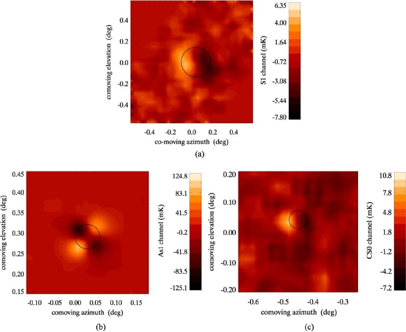
Figure 17: Polarimetry channel response to Jupiter measured with the PIQUE telescope (a) and the CAPMAP telescope (b–c). The data processing to form these maps is described in § 7.1.1 and Figure 14. As detailed in § 8.2, the dipolar and quadrupolar patterns are good examples of spurious polarized signals generated by off-axis and on-axis optical elements respectively. The black circle is the FWHM of the total power beam. Individual panels are on different scales. The peak of the co-polar Jupiter maps is 280 mK for PIQUE and $\sim 3$ K for CAPMAP. The rms noise level is 3 mK for the PIQUE map and 7 mK for both CAPMAP 2003 and CAPMAP 2004 maps. Note that the PIQUE receiver was positioned at the focal point of the telescope, but that the CAPMAP 2003 and CAPMAP 2004 receivers are as far as 15 cm and 48 cm respectively away from the focal point. The magnitude of these spurious responses is summarized in Table 13.

Figure 17 shows the response of representative PIQUE and CAPMAP polarimetry channels to Jupiter, an unpolarized point source (the maps are generated using the same procedures described in § 7.1.1). These maps show patterns dominated by either two or four lobes within the approximate angular scale of the beam. Each map can be fit by a superposition of dipole and quadrupole patterns using the following function:

$$\left[\gamma+d\,\sigma_{y}\frac{\partial}{\partial y}+q\,\sigma_{x}\sigma_{y}\frac{\partial}{\partial x}\frac{\partial}{\partial y}\right]f(x,y),$$ (15)

where $f(x,y)$ is the Gaussian function given in Equation 13, $\sigma_{x}$ and $\sigma_{y}$ are the Gaussian beam widths—which in practice are allowed to float to different values in each term above—and $d$ and $q$ are parameters which quantify the size of the dipole and quadrupole terms, following the conventions used in HHZ. In this formalism, the peak values of the dipole and quadrupole patterns are given by $\pm d/\sqrt{e}$ and $\pm q/e$, where $e$ is the base of natural logarithms.

Unlike $\gamma$, which is sensitive to the characteristics of the polarimeters, $d$ and $q$ are determined predominantly by the optical components of the telescope. The boundary conditions at optically active surfaces are not the same for the two orthogonally polarized components of the incident radiation, which are thus coupled into the polarimeter with slightly different efficiencies depending on the orientation of the incident wave vector (Gans, 1976; Carretti et al., 2004). This effect causes an unpolarized source to generate a spurious polarized signal depending on its position in the sky. For a differencing polarimeter, this spurious signal arises from asymmetries in the beam shapes for the two polarizations (HHZ), while for correlation polarimeters like PIQUE and CAPMAP, these signals are due to non-zero cross-polar beams which couple one polarized component of the incident radiation into the other component at the input to the polarimeter. The electrodynamics behind these two effects are identical and yield the same values of $d$ and $q$ given the same optical elements.

The PIQUE and CAPMAP $d$ and $q$ parameters are summarized in Table 13 and illustrated in Figure 17. PIQUE and CAPMAP demonstrate how the geometry of the optics affects the form of the local contamination, specifically the different patterns generated by on-axis and off-axis optical elements. Theoretically, on-axis systems do not generate a $d$ term because the optical elements do not define a preferred direction relative to the polarization axes. Off-axis systems, by contrast, can generate both $d$ and $q$ terms.

For PIQUE, the dipole term $d\sim-14$ dB clearly dominates. This is to be expected since the corrugations in feed horns are designed explicitly to minimize the leakage terms (Goldsmith, 1998), and the short focal length and strong curvature of the mirror should generate comparatively high amounts of local contamination.

By contrast, in the CAPMAP 2003 system the quadrupolar term $q\sim-8$ dB is roughly 5 dB higher than $d$. This suggests that the contamination generated by the on-axis optical elements (horn and lens) dominates over the contamination produced by the mirrors. Since the correlator takes the product of two electric fields, the power coupled between polarization states should have a peak value of $q^{2}/e^{2}\sim-24$ dB, which is consistent with the measured cross-polar response of the feed system (see Figure 11). Also, the $d$ and $q$ terms of polarimeters with AR grooves on both surfaces of the lenses are twice as big as the terms for the polarimeters with AR grooves on only one surface (see Table 13), and as discussed in § 5.2, we expect grooves to increase the birefringence of the lens surfaces and to compromise the polarization fidelity of the optics (McMahon, 2005). After discovering the high levels of off-axis leakage generated by these lenses, we replaced them before the subsequent observing season with an improved design with very low cross-polarization that produced $d$ and $q$ parameters that were smaller by a factor of 10 (see Table 13).

The dipole and quadrupole leakage terms alias sharp features in the intensity distribution—from the CMB temperature anisotropy or from point sources—into spurious polarization fluctuations. Although this aliasing will be a significant issue for future large arrays (HHZ), it does not pose a significant problem for PIQUE or CAPMAP. PIQUE’s local contamination was sufficiently low that CMB temperature anisotropies, which are roughly 10 times greater than the polarization anisotropies, produced spurious polarized signals more than $6$ dB below the expected E-mode signal. The first season of CAPMAP had higher contamination levels, but the narrow beam width of this experiment only couples spurious CMB temperature signals from higher angular scales, where the temperature anisotropy is strongly damped (HHZ).

8.3 Far Side-Lobe Contamination

Sources far from the optical axis can also produce spurious polarization signals via the far side-lobes of the instrument. The far side-lobes of a telescope are features produced by spillover past the mirrors or scattered radiation from various support structures. These scan-dependent signals have a significant impact on the performance of the experiment because they are synchronous with respect to the scan pattern and are not modulated away like the $1/f$ noise discussed in § 8.1. The effect of these spurious signals on the data quality is detailed in Barkats et al. (2004). The need to remove the scan-synchronous signals effectively reduced the sensitivity of CAPMAP 2003 by a factor of 2. (Note, however, that with the higher sensitivity of the CAPMAP data obtained in later seasons, the impact is smaller.)

In temperature anisotropy experiments, position-dependent signals generated by side-lobes are controlled using ground screens which block radiation from local sources. PIQUE demonstrated that fixed ground screens are not sufficient to control spurious polarized signals. Such fixed ground screens are scanned by sidelobes during the telescope motion and produce scan-synchronous polarized emission for the same reason our miniplate system does. A similar phenomenon was observed in the COMPASS experiment (Farese et al., 2003).

During the first PIQUE observing season, the polarized signal measured at two positions $1^{\circ}$ apart in azimuth differed by hundreds of $\mu$K. This azimuth-dependent offset occurred because the angle of incidence of the radiation reflected off of the fixed ground screens into the polarimeter was different in the different telescope positions, changing the polarized component of the scattered radiation (see § 4.3.2). For PIQUE’s second observing season the inner ground screen was enlarged so that any radiation reflected into the polarimeter would come from this screen and have the same incidence angle regardless of the telescope orientation. With this improved system, the azimuth-dependent signal was reduced by roughly a factor of 2. The remaining signal was due to a small gap between the bottom of the dish and the floor of the inner ground screen enclosure. This gap was closed towards the end of the 2001 season, and the azimuth dependent signals were reduced to $\sim 30~{}\mu$K. These residual signals were constant at the 10% level required for PIQUE, and so no further improvements were needed.

A ground screen was not used in CAPMAP, and during its first observing season, the polarimetry channels registered a scan-synchronous signal (SSS). Note that the level of SSS in CAPMAP was comparable to that in PIQUE, despite the absence of a groundscreen in CAPMAP; this is due to the more aggressive under-illumination in CAPMAP, which effectively uses portions of the mirrors as a co-moving groundscreen. After a second-order polynomial in azimuth was fit to the data in 20 beam-sized azimuth bins and removed, the polarization data from the whole season collapsed into the 20 bins revealed channel-specific SSS with rms levels at 10 $\mu$K–26 $\mu$K. These variations were generated as various side-lobes moved over sources of emission on or near the ground, including the large atmospheric emission near the horizon.

Maps of the side-lobes derived from observations of an RF source have recently been performed, indicating side-lobe features sufficiently strong to cause the observed SSS. More measurements are underway to confirm this interpretation.

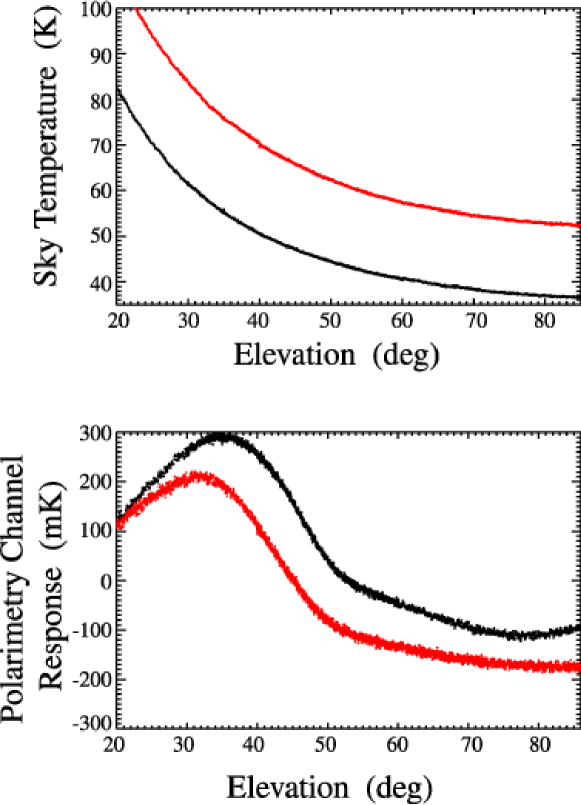
Figure 18: Evidence for polarized side lobes. (top) Change in sky temperature during two elevation scans in 2003 February with a high (gray/red, $T_{z}\sim 50$ K) and a low (black, $T_{z}\sim 35$ K) zenith noise temperature. The sky temperatures are derived from the total power channels by removing the receiver temperature. (bottom) Corresponding polarimetry channels for the same sky dips. The level shift around 45^∘ is consistent with side-lobes due to spillover past the primary moving from the sky to the ground (see § 8.3 for details). A similar level shift is not observed in the total power channels, which indicates that this is not simply monopole leakage of unpolarized signals from the horizon.

An indirect measurement of these side-lobes is found in the elevation scans performed during the first observing season. Since the atmosphere is unpolarized, polarimetry channels should not change as the elevation of the telescope changes (aside from the trend generated by the nonzero $\gamma$). In fact, the level in all the polarimetry channels shifts to a more negative value when the telescope elevation exceeds $\sim 45^{\circ}$ (see Figure 18). The shape of the transition depends on the temperature of the atmosphere and is consistent with side-lobes due to spillover past the primary moving from the sky through the horizon to the ground.

A number of improvements to the optics were made prior to the second season to reduce the size of these side-lobes, including a screen around the secondary and new lenses to sharpen the beam. The results of these modifications will be presented in a later paper.

9 CONCLUSION

The performance of the PIQUE and CAPMAP experiments in the field shows that the concept of the phase-switched correlation polarimeter is well suited for precise CMB polarimetry. We have presented various techniques to improve and evaluate the calibration and systematic effects associated with this type of polarimeter. As the CMB polarization field advances towards higher sensitivities, these techniques will become even more critical. CAPMAP continues to observe the polarized CMB emission with its full set of receivers, and we expect by the summer of 2005 to have increased our observation time with respect to the CAPMAP 2003 data set by an order of magnitude.

Acronym	Meaning
ADC	Analog-to-Digital Converter
AR	Anti-Reflection
CAPMAP	Cosmic Anisotropy Polarization MAPper
CBI	Cosmic Background Imager
CMB	Cosmic Microwave Background
DASI	Degree Angular Scale Interferometer
FWHM	Full Width at Half Maximum
HEMT	High Electron Mobility Transistor
IF	Intermediate Frequency (2–18 GHz at W-band)
LNA	Low Noise Amplifier
LO	Local Oscillator
MMIC	Monolithic Microwave Integrated Circuit
OMT	Ortho-Mode Transducer
PIQUE	Princeton IQU Experiment
PWV	Precipitable Water Vapor
RF	Radio Frequency (84–100 GHz at W-band)
SSS	Scan-Synchronous Signal
WMAP	Wilkinson Microwave Anisotropy Probe

Table 1: Commonly used acronyms

	PIQUE		CAPMAP
Characteristic	W-band	Q-band	W-band	Q-band
$T_{sys}$ (K)	140	50	115	50
Bandwidth (GHz)	11	8	12	8
Sensitivity (mK$\sqrt{\mbox{s}}$)	1.6	0.6	1.3	0.6
No. Detectors	1	1	12	4
Total Sensitivity (mK$\sqrt{\mbox{s}}$)	1.6	0.6	0.4	0.3
Flux Conversion Factor ($\mu$K/Jy)	230	270	3200	6100

Table 2: Typical polarimeter performance parameters for PIQUE and CAPMAP

Component	Gain	Effective Noise	Signal Level	Signal Level
		Temperature	(Polarization)	(Total Power)
Sky + CMB	$\cdots$	$\cdots$	5 $\mu$K	50 K
Lens	$-0.08$ dB	3 K	$1.1\times 10^{-12}~{}\mu$W	$1.1\times 10^{-5}~{}\mu$W
Horn	$<-0.05$ dB	$<0.3$ K	$1.1\times 10^{-12}~{}\mu$W	$1.1\times 10^{-5}~{}\mu$W
OMT	$-0.05$ dB	0.3 K	$1.1\times 10^{-12}~{}\mu$W	$1.1\times 10^{-5}~{}\mu$W
LNAs	35 dB	50 K	$3.5\times 10^{-9}~{}\mu$W	$8.8\times 10^{-2}~{}\mu$W
WG Bend	$-0.3$ dB	$<1$ K	$3.3\times 10^{-9}~{}\mu$W	$8.3\times 10^{-2}~{}\mu$W
Stainless Steel WG	$-0.7$ dB	$<1$ K	$2.8\times 10^{-9}~{}\mu$W	$7.0\times 10^{-2}~{}\mu$W
Filter	$-0.6$ dB	$<1$ K	$2.4\times 10^{-9}~{}\mu$W	$6.0\times 10^{-2}~{}\mu$W
Mixer	$-10$ dB	$<1$ K	$2.4\times 10^{-10}~{}\mu$W	$6.0\times 10^{-3}~{}\mu$W
IF Amplifier	35 dB	3 K	$7.2\times 10^{-7}~{}\mu$W	$18~{}\mu$W
Splitter	$-3$ dB	$\cdots$	$3.6\times 10^{-7}~{}\mu$W	$9~{}\mu$W
Detector Diode	1 mV/$\mu$W	$\cdots$	$\cdots$	3 mV
Filter Bank	$-5$ dB	$\cdots$	$1.2\times 10^{-7}~{}\mu$W	$\cdots$
Multiplier	1.2 mV/$\mu$W	$\cdots$	0.15 nV	$\cdots$
Pre-Amplifier	100	$\cdots$	15 nV	300 mV

Table 3: Summary of W-band polarimeter responsivities and signal levels

Component	W-band Parts	Q-band Parts
OMT	Vertex RSI 111590	Vertex RSI 111588
HEMTP	Custom NRAO	Custom NRAO
HEMTC	Custom JPL	Custom JPL
Filter	MRI FRWS-94	MRI FLQS-40.0
Mixer	Spacek Labs P94-10-LN	Spacek Labs M-40.5-15
LOP	Custom Millimeter Wave	Millimeter Wave 28CSO-30.5
LOC	Spacek GW-820	Spacek GW-305
Power AmpC	Custom JPL	$\cdots$
Phase SwitchP	Pacific Millimeter W180	Pacific Millimeter 2640 MC-30.5
Phase SwitchC	Pacific Millimeter 75MS-82	Pacific Millimeter 2640 MC-30.5
Phase TunerP	Millitech VPS-10-R0000	Millitech VPS-28-S0000
IF AmpP	DBS Microwave DB97-0421	Miteq AFS44-02001800-25-KCR-S-44
IF AmpC	Custom Miteq	Custom Miteq
$0^{\circ}$ Power splitter	MAC Technology P248-2	MAC Technology P248-2
$90^{\circ}$ Hybrid CouplerP	$\cdots$	Sage 2375-9
Detector Diode	Agilent HP 8472-B	Agilent HP 8472-B
Filter Bank	ES Microwave 3SM-7/12.7-10PM	ES Microwave 2SM-9.75-10PM
Phase TunersP	M/A-COM s054-6002-00	Weinschel 917-12
Phase TunersC	Weinschel 917-12	Weinschel 917-12
Multiplier	Miteq DB0218LW2	Miteq DB0218LW2

Table 4: Components list for PIQUE and CAPMAP polarimeters

Component	PIQUE 2000	PIQUE 2001	CAPMAP 2003	CAPMAP 2004
Lens	$\cdots$	$\cdots$	160	130
Horn	40	20	40	25
OMT/LNAs	30	18	40	25
Filters/Mixers	80	50	300	300
LO	315	315	305	315
IF Section	305	305	288	315

Table 5: Operating temperatures of polarimeter components in K

Polarimeter	Channel	LNA	Receiver	Telescope
PIQUE 2000	D0	$\cdots$	73	$\cdots$
	D1	$\cdots$	68	$\cdots$
PIQUE 2001	D0	$\cdots$	66	$\cdots$
	D1	$\cdots$	90	$\cdots$
CAPMAP 2003 A	D0	55	47	80
	D1	53	52	115
CAPMAP 2003 B	D0	53	51	66
	D1	57	46	61
CAPMAP 2003 C	D0	52	53	119
	D1	54	65	76
CAPMAP 2003 D	D0	52	47	72
	D1	55	45	67

Table 6: Radiometer noise temperatures in Kelvin

Polarimeter	$\left\langle\cos\phi\right\rangle$
	S0	S1	S2
PIQUE 2000	0.90	0.91	0.94
PIQUE 2001	0.92	0.93	0.88
CAPMAP 2003 A	0.73	0.90	0.82
CAPMAP 2003 B	0.87	0.90	0.77
CAPMAP 2003 C	0.92	0.90	0.74
CAPMAP 2003 D	0.94	0.82	0.77

Table 7: Radiometer phase statistic $\left\langle\cos\phi\right\rangle$

Parameter	Crawford Hill 7-m Telescope	PIQUE Telescope
Primary Diameter (cm)	700	$140\times 122$
Primary Focal Length $f_{1}$ (cm)	656.59	75
Secondary Diameter (cm)	$120\times 180$	$\cdots$
Secondary Near Focal Length $f_{2}$ (cm)	86.87	$\cdots$
Secondary Far Focal Length $f_{3}$ (cm)	522.62	$\cdots$
Effective Focal Length $f$ (cm)	3945.59	75
Focal Ratio $f/D$	5.63	0.61
Plate Scale (cm$\cdot$deg-1)	68.9	1.30
Horn Aperture Diameter (cm)	2.54	0.980
Horn Length (cm)	11.43	7.62
Beam Width	14.5∘	25∘
Return Loss (dB)	$-50$	$-50$
Lens Diameter (cm)	12.27	$\cdots$
Lens Focal Length (cm)	16.97	$\cdots$
Lens Beam Width	2.3∘	$\cdots$
Lens Reflection (dB)	$-25$	$\cdots$

Table 8: Optical parameters of the PIQUE and CAPMAP telescope systems

Month	Fraction of the time	Average temperature	Average zenith	50% quartile
	the sky is clear	high/low (∘C)	sky temperature (K)	PWV (mm)
Aug	27%	30/20	$\cdots$	$\cdots$
Sep	32%	25/16	$\cdots$	$\cdots$
Oct	$\cdots$	19/9	$\cdots$	12.8
Nov	31%	13/4	$\cdots$	12.8
Dec	40%	6/$-2$	$\cdots$	7.0
Jan	38%	$-3$/$-5$	30	4.0
Feb	46%	5/$-4$	38	4.8
Mar	22%	10/1	48	9.6

Table 9: Atmospheric properties of the Crawford Hill site

Status	PIQUE 2000	PIQUE 2001	CAPMAP 2003
Initial tests and tuning	240	96	384
Post-season tests	840	0	1700
Active observing period	2000	1700	1500
Various electromechanical problems	50	80	150
Scheduled calibration	110	55	60
Planet calibration scans	20	10	20
Bad weather (snow, fog, rain)	910	890	730
CMB observations	810	660	540
CMB data after cuts	310	190	430

Table 10: Time summary (in hours) of the observing seasons

Instrument/Channel	$\theta_{x}$	$\theta_{y}$
PIQUE W-band	$14.27\arcmin\pm 0.28\arcmin$	$13.84\arcmin\pm 0.28\arcmin$
CAPMAP 2003	$3.94\arcmin\pm 0.05\arcmin$	$3.81\arcmin\pm 0.04\arcmin$
CAPMAP 2003 S0	$4.15\arcmin\pm 0.24\arcmin$
CAPMAP 2003 S1	$3.81\arcmin\pm 0.16\arcmin$
CAPMAP 2003 S2	$3.58\arcmin\pm 0.22\arcmin$

Table 11: FWHM beam sizes

Polarimeter	S0	S1	S2	Combined
PIQUE 2000	2.3	2.3	3.4	1.5
CAPMAP 2003 A	3.2	2.1	2.7	1.5
CAPMAP 2003 B	3.4	2.1	2.0	1.3
CAPMAP 2003 C	2.9	2.1	3.5	1.5
CAPMAP 2003 D	3.1	2.2	2.5	1.5

Table 12: Radiometer sensitivities in thermodynamic units (mK$\sqrt{\mbox{s}}$)

Parameter	PIQUE	CAPMAP 2003		CAPMAP 2004
	no lens	double AR	single AR	optimized
$\gamma$	$-23$ dB	$-23$ dB		$-23$ dB
$d$	$-14$ dB	$-11$ dB	$-15$ dB	$\leq-21$ dB
$q$	$\cdots$	$-7$ dB	$-10$ dB	$\leq-19$ dB

Table 13: Typical leakage terms for the PIQUE and CAPMAP experiments

References

- Barkats (2004) Barkats, D. 2004, PhD thesis, Princeton University
- Barkats et al. (2004) Barkats, D., et al. 2004, ApJ, 619, L127
- Barnes et al. (2002) Barnes, C., et al. 2002, ApJS, 143, 567
- Bennett et al. (2003a) Bennett, C. L., et al. 2003a, ApJS, 148, 1
- Bennett et al. (2003b) Bennett, C. L., et al. 2003b, ApJS, 148, 97
- Carretti et al. (2004) Carretti, E., Cortiglioni, S., Sbarra, C., & Tascone, R. 2004, A&A, 420, 437
- Chu et al. (1978) Chu, T. S., Wilson, R. W., England, D. A., & Legg, W. E. 1978, Bell System Technical Journal, 57, 1257
- Church et al. (2003) Church, S., et al. 2003, New A Rev., 47, 1083
- Cortiglioni (1994) Cortiglioni, S. 1994, Rev. Sci. Instrum., 65, 2667
- de Pater (1999) de Pater, I. 1999, Encyclopedia of the Solar System (Academic Press), 735–772
- Farese et al. (2003) Farese, P. C., et al. 2003, New A Rev., 47, 1033
- Farese et al. (2004) —. 2004, ApJ, 610, 625
- Gaier et al. (2003) Gaier, T., Lawrence, C. R., Seiffert, M. D., Wells, M. M., Kangaslahti, P., & Dawson, D. 2003, New A Rev., 47, 1167
- Gans (1976) Gans, M. J. 1976, Bell System Technical Journal, 55(3), 289
- Goldsmith (1998) Goldsmith, P. F. 1998, Quasioptical Systems: Gaussian Beams Quasioptical Propagation and Applications (IEEE Press)
- Hamaker et al. (1996) Hamaker, J. P., Bregman, J. D., & Sault, R. J. 1996, A&AS, 117, 137
- Hanany & Rosenkranz (2003) Hanany, S., & Rosenkranz, P. 2003, New A Rev., 47, 1159
- Hedman (2002) Hedman, M. M. 2002, PhD thesis, Princeton University
- Hedman et al. (2002) Hedman, M. M., Barkats, D., Gundersen, J. O., McMahon, J. J., Staggs, S. T., & Winstein, B. 2002, ApJ, 573, L73
- Hedman et al. (2001) Hedman, M. M., Barkats, D., Gundersen, J. O., Staggs, S. T., & Winstein, B. 2001, ApJ, 548, L111
- Heiles et al. (2001) Heiles, C., et al. 2001, PASP, 113, 1274
- Hu et al. (2003) Hu, W., Hedman, M. M., & Zaldarriaga, M. 2003, Phys. Rev. D, 67, 043004
- Huei et al. (2001) Huei, W., et al. 2001, IEEE Trans. Microwave Theory Techniques, 49, 9
- IAU (1973) IAU. 1973, Trans. IAU, 15B, 166
- Imbriale (2003) Imbriale, W. A. 2003, Large Antennas of the Deep Space Network (Wiley and Sons)
- Imbriale & Hodges (1991) Imbriale, W. A., & Hodges, R. E. 1991, Applied Computational Electromagnectic Society Journal, 6, 74
- Jackson (1998) Jackson, J. D. 1998, Classical Electrodynamics, 3rd edn. (Wiley)
- James (1981) James, G. L. 1981, IEEE Trans. Microwave Theory Techniques, 29, 1059
- Jarosik et al. (2003) Jarosik, N., et al. 2003, ApJS, 145, 413
- Johnson et al. (2003) Johnson, B. R., et al. 2003, New A Rev., 47, 1067
- Kamionkowski & Kosowsky (1998) Kamionkowski, M., & Kosowsky, A. 1998, Phys. Rev. D, 57, 685
- Keating et al. (1998) Keating, B., Timbie, P., Polnarev, A., & Steinberger, J. 1998, ApJ, 495, 580
- Keating et al. (2003) Keating, B. G., et al. 2003, in Polarimetry in Astronomy, ed. S. Fineschi, Vol. 4843 (SPIE), 284–295
- Kovac et al. (2002) Kovac, J. M., Leitch, E. M., Pryke, C., Carlstrom, J. E., Halverson, N. W., & Holzapfel, W. L. 2002, Nature, 420, 772
- Kraus (1986) Kraus, J. D. 1986, Radio Astronomy (Cygnus Quaasar Books)
- Leitch et al. (2002) Leitch, E. M., et al. 2002, Nature, 420, 763
- Leitch et al. (2004) —. 2004, ApJ, submitted, arXiv: astro-ph/0409357
- Mayer & Hollinger (1968) Mayer, C. H., & Hollinger, J. P. 1968, ApJ, 151, 53
- McMahon (2005) McMahon, J. J. 2005, in preparation
- Montroy et al. (2003) Montroy, T., et al. 2003, New A Rev., 47, 1057
- O’dell (2002) O’dell, C. 2002, PhD thesis, University of Wisconsin, arXiv: astro-ph/0201224
- Page et al. (2003) Page, L., et al. 2003, ApJS, 148, 39
- Pozar (1998) Pozar, D. M. 1998, Microwave Engineering, 2nd edn. (Wiley and Sons)
- Readhead et al. (2004) Readhead, A. C. S., et al. 2004, Science, 306, 836
- Rohlfs & Wilson (1996) Rohlfs, K., & Wilson, T. L. 1996, Tools of Radio Astronomy, 2nd edn. (Springer-Verlag)
- Seljak & Hirata (2004) Seljak, U., & Hirata, C. M. 2004, Phys. Rev. D, 69, 043005
- Seljak & Zaldarriaga (1997) Seljak, U., & Zaldarriaga, M. 1997, Phys. Rev. Lett., 78, 2054
- Seljak & Zaldarriaga (1999) —. 1999, Phys. Rev. D, 60, 043504
- Smith et al. (2004) Smith, K. M., Hu, W., & Kaplinghat, M. 2004, Phys. Rev. D, 70, 043002
- Staggs et al. (2002) Staggs, S. T., Barkats, D., Gundersen, J. O., Hedman, M. M., Herzog, C. P., McMahon, J. J., & Winstein, B. 2002, in AIP Conf. Proc. 609: Astrophysical Polarized Backgrounds, 183–186
- Strozzi & McDonald (2000) Strozzi, D. J., & McDonald, K. T. 2000, arXiv: physics/0005024
- Tegmark et al. (2000) Tegmark, M., Eisenstein, D. J., Hu, W., & de Oliveira-Costa, A. 2000, ApJ, 530, 133
- Tinbergen (1996) Tinbergen, J. 1996, Astronomical Polarimetry (Cambridge University Press)
- Weinreb et al. (1999) Weinreb, S., Lai, R., Erickson, N., Gaier, T., & Wielgus, J. 1999, IEEE MTT-S International, 1, 101
- Wollack et al. (1997) Wollack, E. J., Devlin, M. J., Jarosik, N., Netterfield, C. B., Page, L., & Wilkinson, D. 1997, ApJ, 476, 440
- Zaldarriaga & Seljak (1998) Zaldarriaga, M., & Seljak, U. 1998, Phys. Rev. D, 58, 023003
- Zhang (1993) Zhang, X. 1993, IEEE Trans. Microwave Theory Techniques, 41(8), 1263