The Relationship between Class I and Class II Methanol Masers

Abstract

The Australia Telescope National Facility Mopra millimetre telescope has been used to search for 95.1-GHz class I methanol masers towards sixty-two 6.6-GHz class II methanol masers. A total of twenty-six 95.1-GHz masers were detected, eighteen of these being new discoveries. Combining the results of this search with observations reported in the literature, a near complete sample of sixty-six 6.6-GHz class II methanol masers has been searched in the 95.1-GHz transition, with detections towards 38 per cent (twenty-five detections ; not all of the sources studied in this paper qualify for the complete sample, and some of the sources in the sample were not observed in the present observations).

There is no evidence of an anti-correlation between either the velocity range, or peak flux density of the class I and II transitions, contrary to suggestions from previous studies. The majority of class I methanol maser sources have a velocity range that partially overlaps with the class II maser transitions. The presence of a class I methanol maser associated with a class II maser source is not correlated with the presence (or absence) of main-line OH or water masers. Investigations of the properties of the infrared emission associated with the maser sources shows no significant difference between those class II methanol masers with an associated class I maser and those without. This may be consistent with the hypothesis that the objects responsible for driving class I methanol masers are generally not those that produce main-line OH, water or class II methanol masers.

1 Introduction

Intense activity in the field of methanol maser research commenced in the mid 1980s with the discovery of numerous new transitions (e.g. Morimoto et al., 1985; Wilson et al., 1984, 1985, and others). As the number of methanol maser transitions increased it became clear that they could be classified empirically into two groups on the basis of the sources towards which they were detected (Batrla et al., 1987; Menten, 1991a). Class II methanol masers are found close to sites of high-mass star formation and are often associated with Hii regions, infrared sources and OH masers. The strongest and most widespread class II transitions are the $5_{1}-6_{0}\mbox{A}^{+}$ (6.6 GHz) and $2_{0}-3_{-1}\mbox{E}$ (12.1 GHz), which have been detected towards more than 500 sites within the Galaxy (Pestalozzi, Minier & Booth, 2004, and references therein). The archetypal class II methanol maser source is W3(OH). Class I methanol masers are also found towards star formation regions, but offset by small, though significant amounts from Hii regions, infrared sources, OH and water masers. The strongest class I transitions are the $7_{0}-6_{1}\mbox{A}^{+}$ (44.0 GHz) and $4_{-1}-3_{0}\mbox{E}$ (36.1 GHz), and the archetypal source is Orion KL. The class II $2_{0}-3_{-1}\mbox{E}$ transition is often observed in absorption towards class I sources (Peng & Whiteoak, 1992). Theoretical models of methanol masers provide some explanation for this empirical division predicting inversion in the class I transitions when collisional processes dominate and inversion in the class II transitions when radiative processes dominate (Cragg et al., 1992; Sobolev & Deguchi, 1994; Sobolev, Cragg & Godfrey, 1997).

The classification suggested by Menten (1991a) was consistent with the observational and theoretical understanding at the time. However, more recent studies suggest that things may be more complicated. A number of searches for class I methanol masers have been made towards traditional class II sites with relatively high detection rates (Slysh et al., 1994; Val’tts et al., 2000). Slysh et al. (1994) suggested an anti-correlation between the intensities and velocity ranges of the class I and II methanol masers within the same region. This requires that there is some sort of relationship between the emission from the two transitions since, if they were independent neither correlations, nor anti-correlations should exist. Perhaps more importantly, modelling predicts that in some conditions the 6.6-GHz class II transition can be weakly inverted, simultaneously with strong inversion in the 25-GHz class I transitions. This situation may have recently been detected towards the archetypal class I maser source Orion KL (Voronkov et al., 2004). Kurtz, Hofner & Álvarez (2004) found coincidence within 0.5 arcsec of class I and II methanol masers in one source, although there is a significant velocity difference between the two transitions suggesting that it may be a chance alignment along our line of sight.

The majority of studies of methanol masers have focused upon the class II transitions. There are two main reasons for this ; the first is that the strongest class II transitions are in the centimetre regime and hence easier to observe ; the second is that their association with other maser species, IRAS sources etc makes targeted searches relatively productive (e.g. Menten, 1991b; Caswell et al., 1995b; Walsh et al., 1997). Although untargeted searches have also been very successful at detecting class II methanol masers (Caswell, 1996; Ellingsen et al., 1996; Szymczak et al., 2002). In contrast the strongest class I methanol maser transitions are at millimetre wavelengths and to date there is no other type of astrophysical object with which they are known to be closely associated. Menten (1991a) suggested that class I masers are offset from class II sites by up to 1 pc. However, there are relatively few sources where both class I and II transitions have been imaged at high resolution. The majority of the well studied class I methanol maser sources are “traditional” class I sources with no (or weak) class II emission, Orion KL (Plambeck & Wright, 1988; Johnston et al., 1992), DR21 (Batrla & Menten, 1988; Plambeck & Menten, 1990) and Sgr B2 (Mehringer & Menten, 1997). There are no strong class II methanol masers towards Orion KL, although weak masers, and possibly quasi-thermal emission has been detected Voronkov et al. (2004). There is class II methanol maser emission towards DR21(OH), this likely to be from the same region as the OH maser emission (which is offset from the class I masers), but this has not been confirmed. Sgr B2 is a very complex region, with multiple site of both class I and II methanol masers. The class II masers are close to the compact Hii regions Houghton & Whiteoak (1995), while the majority of class I masers lie in an arc, possibly tracing the interface between two molecular clouds Mehringer & Menten (1997).

For a source at a distance of 3 kpc (typical for a high-mass star forming region) a linear distance of 1 pc corresponds to an angular separation of slightly more than 1 arcminute. This is comparable to, or larger than typical telescope beam sizes at millimetre wavelengths and so searches targeted at class II maser sites (e.g. Slysh et al., 1994; Val’tts et al., 2000) would be expected to detect few class I sources. This is not the case though, which suggests that in many cases the offset between class I and II maser sites is significantly less than 1 pc. This has been confirmed by recent VLA observations of 44 GHz class I methanol masers (Kurtz et al., 2004) which found a median separation of 0.2 pc from Hii regions. At the present time, class II methanol maser sites appear to be the best targets for class I maser searches. However, the nature of the relationship between the two classes remains unclear. To try and elucidate the nature of the relationship I have undertaken a search for class I methanol masers towards a statistically complete sample of class II methanol masers selected from the Mt Pleasant survey (Ellingsen et al., 1996; Ellingsen, 1996).

2 Observations and Data reduction

The observations were made between 1998 July 12–17 using the Australia Telescope National Facility (ATNF) 22m millimetre antenna at Mopra. At the time of the observations only the inner 15 m of the Mopra antenna was illuminated and the antenna had a sensitivity of approximately 40 Jy K^-1. The assumed rest frequency of the $8_{0}-7_{1}\mbox{A}^{+}$ was 95.169 489 GHz (De Lucia et al., 1989) and at this frequency the half-power beam width of the Mopra antenna was 52 arcsec. Recent measurement of the rest frequencies of various methanol maser transitions by Müller, Menten & Mäder (2004) gives a value of 95.169 463 GHz (with an uncertainty of 10 kHz). This is 14 kHz lower than the value used, which means that the velocities listed are 0.044 $\mbox{km~{}s}^{-1}$ higher than had the more recent rest frequency value been used. The data were collected using a 2-bit digital autocorrelation spectrometer configured with 1024 channels spanning a 32-MHz bandwidth. For an observing frequency of 95.1 GHz this configuration yields a natural weighting velocity resolution of 0.12 $\mbox{km~{}s}^{-1}$, or 0.2 $\mbox{km~{}s}^{-1}$after Hanning smoothing. The SIS mixers on both of the available linear polarization channels were tuned to the 95.1 GHz methanol transition. The antenna pointing was checked and corrected prior to each observing session by making observations of 86-GHz SiO masers; the nominal pointing accuracy is of the order of 10 arcsec RMS. For one of the channels the tuning was performed only once at the beginning of the observing period. However, the other channel had to be re-tuned each day after the pointing checks. The sensitivity of this channel varied day to day depending upon how well the receiver tuned, in general it had a system temperature approximately 50K higher than the other channel, though on occasions it was slightly lower. The system temperature was determine by inserting an ambient temperature load which was assumed to have a temperature of 295K. The measured system temperature varied between 200 and 340K depending upon the weather conditions and elevation. This method of calibration also corrects for atmospheric absorption (Kutner & Ulich, 1981) and taking into account pointing inaccuracies the absolute accuracy of the flux density scale of the observations is conservatively estimated to be 20 per cent. The sources were observed in a position switching mode with 300 seconds spent at the on-source position and 300 seconds at a reference position offset in declination 30 arcminutes to the south. This procedure was repeated 3 times to yield a total on-source integration time of 15 minutes for most sources, which typically yielded an RMS of 1.3 Jy after averaging the two polarizations and Hanning smoothing. Wiesemeyer, Thum & Walmsley (2004) recently observed linear polarization in excess of 10% in a number of class I methanol maser transitions, including the 95.1-GHz. The spectra presented here are an average of two orthogonal linear polarizations and hence the relative flux density of the features will not be effected by any linear polarization. The current observations were made in such a way that it is not possible to determine the polarization characteristics of the masers from them. The data were processed using the spc reduction package. Quotient spectra were formed for each on/off pair of observations which were then averaged together, a polynomial baseline fitted and subtracted and the velocity and amplitude scale calibrated. Velocity calibration presented some challenges, requiring correction for incorrectly recorded frequency synthesiser chain information in the RPFITS header Ladd et al. (2004) and editing of the telescope identity and band-inversion in the headers.

The sample of 6.6-GHz methanol maser sites searched for 95.1-GHz maser emission was drawn from Ellingsen et al. (1996) and Ellingsen (1996) and included all sources detected in the regions with Galactic longitude $l=25^{\circ}$ – $30^{\circ},282^{\circ}$ – $286^{\circ},291^{\circ}$ – $296^{\circ},325^{\circ}$ – $335^{\circ}$. For the first and last of these longitude ranges the Galactic latitude range of the Mt Pleasant survey was $b=-0\aas@@fstack{\circ}53$ – $+0\aas@@fstack{\circ}53$, while for the other regions it was $b=-1\aas@@fstack{\circ}03$ – $+0\aas@@fstack{\circ}03$. The total area covered is approximately 24.4 square degrees. The exact number of class II methanol masers sites within these regions depends on the spatial resolution of the observations. A number of the sources have two or more sites of emission separated by a few arcseconds. Such sources cannot be resolved with the Mopra telescope and so in general we have made observations towards individual sites only where they are separated by more than 20 arcsec. Observations of the 95.1-GHz transition were made of a small number of sources not detected as part of the original Mt Pleasant survey. In particular, $326.475\!+0\!.703$ which was listed as $326.40\!+\!0.51$ in the original survey (Ellingsen et al., 1996), the correct position being revealed by Australia Telescope Compact Array (ATCA) observations. $27.286\!+\!0.151$ is outside the velocity range of the Mt Pleasant survey, but was discovered during ATCA observations of the nearby source $27.223\!+\!0.137$. In addition, the untargeted search of Caswell (1996) detected a number of 6.6-GHz methanol masers in the region $l=330^{\circ}-335^{\circ}$ which were not detected in the Mt Pleasant survey either due to variability or being outside the searched velocity range ($331.120\!-\!0.118$, $333.029\!-\!0.063$, $333.646\!+\!0.058$ & $334.935\!-\!0.098$) and these were also searched for 95.1-GHz methanol masers. An independent untargeted survey of the $l=20^{\circ}-40^{\circ}$ region has recently been undertaken with the Torun telescope (Szymczak et al., 2002), which also discovered a number of sources in the $l=25^{\circ}-30^{\circ}$ region not detected at Mt Pleasant. However these were not searched as the information was not available at the time of the observations. For the majority of sources (80 of 84) the positions search for 95.1-GHz class I methanol masers are the sites of class II masers determined from ATCA observations which have a positional accuracy of approximately 0.5 arcsec (Ellingsen, unpublished observations). The only exceptions were the sources $285.32\!-\!0.03$, $293.84\!-\!0.78$, $293.95\!-\!0.91$ and $25.53\!+\!0.38$, for which the positions determined in the Mt Pleasant survey (positional accuracy RMS 0.6 arcmin) were used (Ellingsen et al., 1996). For those sources where ATCA position are available we have used three significant figures for the Galactic coordinate names. These names differ slightly from those used previously in the literature, but the greater accuracy of the ATCA positions warrants it, and the correspondence is in most cases reasonably obvious.

A small number of the detected 95.1-GHz methanol masers were either not observed, or have poor spectra from the original 6.6-GHz Mt Pleasant survey. To enable proper comparison of the class I and class II emission in all class I detections, new 6.6-GHz observations were made of the sources 326.474$\!+\!$0.703, 333.029$\!-\!$0.063 and 27.286$\!+\!$0.151. These observations were made with the Mt Pleasant 26-m telescope on 2004 November 3 & 8. The assumed rest frequency of the $5_{1}-6_{0}\mbox{A}^{+}$ transition was 6.668518 GHz, and at this frequency the half-power beam width of the Mt Pleasant antenna is 7 arcmin. The observations were made with a cryogenically cooled receiver with dual circular polarizations and a system equivalent flux density of approximately 1200 Jy. The data were collected using a 2-bit autocorrelation spectrometer configured with 4096 channels spanning a 4-MHz bandwidth for each polarizations. For an observing frequency of 6.6-GHz this configuration yields a velocity resolution after Hanning smoothing of 0.09 $\mbox{km~{}s}^{-1}$. Each source was observed in position switching mode with 10 minutes spent at the on-source position and a further 10 minutes at a reference position offset by -1 degree in declination. To measure any pointing errors a 5-point grid, centred on the nominal position was observed for each source. In each case the measured pointing offsets were small, implying scaling corrections to the flux density scale of the source spectra of less than 5 per cent. As this is less than the accuracy of the flux density calibration, no scaling was applied.

3 Results

A total of fifty-nine 6.6-GHz class II methanol maser sites were searched for 95.1 GHz class I masers. Emission was detected towards twenty-six sites and these are listed, along with the parameters of Gaussian fits to the emission in Table 1. Spectra of each of the detected 95.1-GHz masers are shown in Figure 1. Eighteen of the 95.1-GHz emission sites detected are new discoveries, with the remainder previously observed by Val’tts et al. (2000). The sources for which no emission was detected are listed in Table 3, along with the velocity range searched and the 3$\sigma$ detection limit for the observation.

Table 1: Class II methanol maser sites detected in the 95.1-GHz class I transition. The Hanning smoothed spectra have been fitted with one or more Gaussian profiles and the fitted parameters are listed, the number in brackets is the uncertainty reported by the fitting procedure. Notes : ^a sources not within the statistically complete sample of 6.6-GHz methanol masers.

Name	Right Ascension	Declination	Peak Flux	Velocity	Full Width
	(J2000)	(J2000)	Density	($\mbox{km~{}s}^{-1}$)	Half Maximum
	(h m s)	(∘ ′ ″)	(Jy)		($\mbox{km~{}s}^{-1}$)
$328.237\!-\!0.548^{a}$	15:57:58.381	-53:59:23.14	5.2(1.3)	-41.8(0.1)	1.6(0.3)
			4.4(0.8)	-41.3(0.05)	0.4(0.1)
			3.8(0.5)	-44.0(0.2)	2.2(0.3)
			2.3(0.4)	-39.7(0.9)	3.9(1.3)
$328.809\!+\!0.633^{a}$	15:55:48.608	-52:43:06.20	18.3(1.6)	-40.9(0.1)	1.5(0.1)
			17.3(1.4)	-41.4(0.05)	5.2(0.2)
			14.1(1.2)	-40.5(0.05)	0.4(0.05)
			13.9(1.1)	-42.6(0.05)	1.3(0.1)
$329.031\!-\!0.198$	16:00:30.326	-53:12:27.35	13.4(1.0)	-47.0(0.05)	0.7(0.1)
			12.0(1.9)	-43.9(0.1)	1.3(0.2)
			8.0(0.5)	-46.0(0.2)	2.4(0.3)
			6.7(2.4)	-43.5(0.1)	1.2(0.3)
			5.7(2.0)	-43.7(0.05)	0.4(0.2)
			4.4(0.6)	-41.6(0.6)	4.4(0.9)
$331.132\!-\!0.244$	16:10:59.743	-51:50:22.70	31.6(0.6)	-91.1(0.05)	0.8(0.05)
			8.8(0.7)	-88.5(0.05)	0.5(0.1)
			8.4(0.2)	-86.7(0.1)	6.9(0.2)
			5.6(0.6)	-84.6(0.05)	0.8(0.1)
$331.342\!-\!0.346$	16:12:26.456	-51:46:16.86	12.9(0.7)	-65.8(0.05)	0.6(0.05)
$332.295\!-\!0.094$	16:15:45.381	-50:55:53.85	14.5(5.4)	-50.8(0.05)	0.5(0.1)
$332.942\!-\!0.686^{a}$	16:21:19.018	-50:54:10.41	4.6(0.4)	-48.6(0.1)	3.6(0.3)
			3.8(0.7)	-49.0(0.1)	0.7(0.2)
$332.963\!-\!0.679^{a}$	16:21:22.926	-50:52:58.71	9.1(0.7)	-46.8(0.05)	0.6(0.1)
			8.5(1.0)	-47.4(0.05)	0.5(0.1)
			3.0(0.3)	-49.0(0.2)	4.4(0.5)
$333.029\!-\!0.063^{a}$	16:18:56.735	-50:23:54.17	3.7(1.0)	-41.0(0.1)	0.4(0.1)
			2.8(0.5)	-40.1(0.1)	1.0(0.3)
$333.121\!-\!0.434$	16:20:59.704	-50:35:52.32	6.1(0.2)	-50.9(0.1)	7.1(0.2)
			6.0(0.5)	-52.9(0.05)	0.9(0.1)
			5.3(0.7)	-50.7(0.05)	0.4(0.1)
$333.128\!-\!0.440$	16:21:03.300	-50:35:49.75	23.3(0.7)	-47.6(0.05)	2.7(0.1)
			21.9(1.2)	-48.6(0.05)	1.2(0.1)
			9.2(0.8)	-49.9(0.1)	2.0(0.2)
			7.4(0.4)	-50.6(0.2)	7.1(0.4)
$333.130\!-\!0.560^{a}$	16:21:35.742	-50:40:51.29	7.6(0.6)	-59.1(0.05)	1.4(0.1)
			6.4(0.6)	-54.4(0.05)	0.5(0.1)
			4.6(0.2)	-56.5(0.2)	3.8(0.4)
$333.163\!-\!0.101^{a}$	16:19:42.670	-50:19:53.20	3.7(0.5)	-91.3(0.05)	0.6(0.1)
			3.5(0.7)	-109.8(0.05)	0.5(0.1)
$333.184\!-\!0.091$	16:19:45.620	-50:18:35.00	4.4(1.8)	-87.0(0.1)	0.2(0.2)
			4.3(0.8)	-86.5(0.1)	1.4(0.3)
$333.234\!-\!0.062$	16:19:51.250	-50:15:14.10	131.9(0.9)	-87.3(0.05)	1.1(0.05)
			17.7(0.8)	-87.6(0.05)	4.0(0.1)
$333.315\!+\!0.105$	16:19:29.016	-50:04:41.45	2.5(0.3)	-46.5(0.3)	3.5(0.8)
			2.2(0.8)	-44.4(0.2)	1.0(0.5)
$333.466\!-\!0.164$	16:21:20.180	-50:09:48.60	7.5(0.4)	-42.9(0.1)	3.0(0.2)
			5.1(0.7)	-45.2(0.05)	0.5(0.1)
			4.7(0.8)	-42.8(0.05)	0.4(0.1)
$333.562\!-\!0.025$	16:21:08.797	-49:59:48.26	11.8(1.6)	-40.0(0.1)	0.6(0.1)
			6.7(1.9)	-39.4(0.1)	0.6(0.2)
			4.3(1.5)	-40.1(0.2)	2.1(0.4)
$335.060\!-\!0.427^{a}$	16:29:23.146	-49:12:27.34	2.9(0.5)	-39.3(0.1)	2.9(0.4)
			1.7(0.8)	-39.2(0.1)	0.4(0.3)
$25.826\!-\!0.178$	18:39:03.621	-06:24:09.29	53.8(1.0)	90.2(0.05)	0.4(0.05)
			15.4(1.0)	98.4(0.05)	0.7(0.05)
			10.0(1.0)	91.7(0.05)	0.3(0.05)
			9.8(0.4)	94.2(0.1)	4.3(0.3)
			4.6(0.7)	91.4(0.1)	2.5(0.3)
			1.7(0.9)	98.5(0.4)	1.4(0.9)
$26.602\!-\!0.220$	18:40:38.550	-05:43:56.20	8.3(1.6)	108.0(0.05)	0.3(0.1)
			2.8(0.7)	106.8(0.2)	1.0(0.6)

Table 2: continued

Name	Right Ascension	Declination	Peak Flux	Velocity	Full Width	Ref
	(J2000)	(J2000)	Density	($\mbox{km~{}s}^{-1}$)	Half Maximum
	(h m s)	(∘ ′ ″)	(Jy)		($\mbox{km~{}s}^{-1}$)
$27.286\!+\!0.151^{a}$	18:40:34.476	-04:57:13.44	3.6(0.4)	31.6(0.05)	0.8(0.1)	*
			3.1(0.5)	33.1(0.05)	0.5(0.1)
$27.369\!-\!0.164$	18:41:50.982	-05:01:28.23	22.9(0.8)	95.3(0.05)	0.5(0.05)	*
			20.2(0.9)	93.7(0.1)	1.8(0.1)
			13.7(1.4)	94.2(0.05)	0.5(0.1)
			6.2(0.4)	92.0(0.1)	7.0(0.3)
			5.8(0.6)	90.6(0.05)	0.6(0.1)
			4.1(0.7)	92.1(0.05)	0.4(0.1)
$28.303\!-\!0.389$	18:44:22.056	-04:17:48.84	4.7(1.0)	74.0(0.05)	0.2(0.1)	*
$29.907\!-\!0.040$	18:46:03.585	-02:42:36.34	26.6(1.0)	98.2(0.05)	0.3(0.05)	*
$29.974\!-\!0.029$	18:46:08.505	-02:38:42.66	3.1(0.6)	96.4(0.1)	0.5(0.2)	1
			2.2(0.8)	97.0(0.1)	0.4(0.2)

Figure 1: Spectra of the 95.1-GHz class I methanol maser sources (top) and the corresponding 6.6-GHz class II methanol masers (bottom). The 95.1-GHz spectra are from the current work, except for those sources where Val’tts et al. (2000) is the only reference listed in Table 4. The 6.6-GHz spectra are from either Ellingsen et al. (1996), Ellingsen (1996) or the current work, as listed in the relevant column of Table 4. All 95.1-GHz spectra have been Hanning smoothed.

Figure 2: continued

Figure 3: continued

Figure 4: continued

Figure 5: continued

Table 3: Class II methanol maser sites not detected in the 95.1-GHz class I transition. The RMS noise level listed is that measured in the Hanning smoothed spectra. Notes : ^a sources not within the statistically complete sample of 6.6-GHz methanol masers, ^b emission detected towards this source, but it appears to be a sidelobe response to 29.907-0.040.

Name	R.A.(J2000)	Dec.(J2000)	Velocity Range	3$\sigma$
	(h m s)	(∘ ′ ″)	($\mbox{km~{}s}^{-1}$)	(Jy)
$327.120\!+\!0.511$	15:47:32.729	-53:52:38.90	-120 – -55	4.4
$327.401\!+\!0.445$	15:49:19.4	-53:45:14	-122 – -46	4.2
$327.402\!+\!0.444$	15:49:19.523	-53:45:14.21	-122 – -46	4.2
$327.590\!-\!0.094$	15:52:36.824	-54:03:18.97	-122 – -46	4.8
$329.407\!-\!0.459$	16:03:32.662	-53:09:26.98	-105 – -29	4.2
$330.952\!-\!0.182^{a}$	16:09:52.372	-51:54:57.89	-127 – -50	4.2
$331.278\!-\!0.188$	16:11:26.596	-51:41:56.67	-118 – -40	3.8
$331.542\!-\!0.066$	16:12:09.020	-51:25:47.60	-124 – -47	3.8
$331.556\!-\!0.121^{a}$	16:12:27.210	-51:27:38.20	-143 – -66	4.1
$333.029\!-\!0.015$	16:18:44.167	-50:21:50.77	-92 – -16	3.0
$333.068\!-\!0.447$	16:20:48.995	-50:38:40.72	-92 – -16	3.4
$333.646\!+\!0.058^{a}$	16:21:09.140	-49:52:45.90	-127 – -50	3.8
$333.683\!-\!0.437$	16:23:29.794	-50:12:08.69	-45 – 32	3.3
$333.931\!-\!0.135$	16:23:14.831	-49:48:48.87	-76 – 0	4.1
$334.635\!-\!0.015$	16:25:45.729	-49:13:37.51	-70 – 7	3.2
$334.935\!-\!0.098^{a}$	16:27:24.250	-49:04:11.30	-67 – 20	3.0
$25.411\!+\!0.105$	18:37:16.918	-06:38:28.23	58 – 136	4.2
$25.386\!+\!0.005$	18:37:35.522	-06:42:34.34	56 – 132	3.9
$25.53\!+\!0.38$	18:36:32.6	-06:24:26	52 – 130	3.7
$25.710\!+\!0.044$	18:38:03.097	-06:24:14.31	56 – 132	4.1
$26.528\!-\!0.266$	18:40:40.227	-05:49:07.67	66 – 142	4.0
$27.223\!+\!0.137$	18:40:30.434	-05:00:58.88	80 – 156	3.0
$28.151\!-\!0.002$	18:42:42.494	-04:15:18.34	62 – 138	3.1
$28.829\!+\!0.488$	18:42:12.433	-03:25:39.56	46 – 122	3.2
$28.863\!-\!0.237$	18:44:51.000	-03:43:44.17	50 – 126	3.3
$28.810\!+\!0.360$	18:42:37.485	-03:30:12.52	56 – 130	3.4
$29.313\!-\!0.165$	18:45:24.974	-03:17:44.47	6 – 82	3.4
$29.867\!-\!0.042$	18:45:59.530	-02:44:47.23	56 – 132	3.5
$29.865\!-\!0.007$	18:45:51.765	-02:43:57.38	52 – 128	3.5
$29.895\!-\!0.047^{b}$	18:46:03.653	-02:43:24.89	60 – 136	3.1
$29.918\!-\!0.035^{b}$	18:46:03.690	-02:41:52.53	60 – 136	2.9
$29.923\!+\!0.059$	18:45:44.184	-02:39:03.71	60 – 136	3.1
$30.009\!-\!0.017$	18:46:09.851	-02:36:30.75	60 – 136	3.4

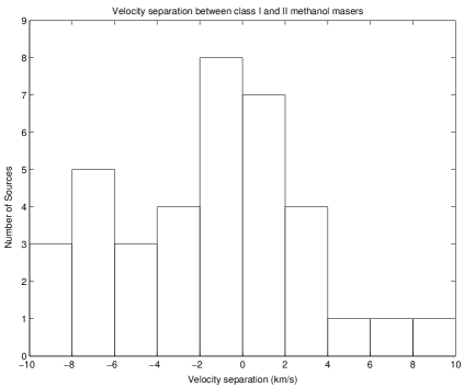
Figure 7: The difference between the velocity ranges of the class I 95.1-GHz methanol masers and the corresponding class II 6.6-GHz transition. A negative value indicates that the emission from the two classes overlaps.

The primary purpose of these observations was to realise a search for 95.1-GHz class I methanol masers towards a statistically complete sample of 6.6-GHz class II methanol masers. Table 4 gives the intensity and velocity of the peak flux density and the velocity range for both the class I and class II methanol masers for all the 6.6-GHz masers detected in the Mt Pleasant survey (not just those in the statistically complete sample) and the additional sources listed in section 2. There are two 6.6-GHz class II methanol maser sources from the statistically complete sample which were accidentally omitted from the sources searched for 95.1-GHz class I masers ($328.254\!-\!0.254$ & $28.201\!-\!0.049$). The data for the class II emission in these sources is included in Table 4. Fortunately the omission of two of sixty-eight sources does not significantly effect the reported statistics or conclusions of this study. For sources where both classes of methanol maser were detected spectra of each are shown on a common velocity scale in Figure 1. Many of the class II methanol maser spectra contain emission from multiple sources, present within a single Mt Pleasant beam (7 arcmin at 6.6 GHz). Where this occurs the emission from the nearby sources is indicated in the spectra. Examination of Fig. 1 shows that the peaks of the two classes of methanol masers essentially never coincide in velocity. The median difference between the peak velocity of the class I and class II transitions is 3.6 $\mbox{km~{}s}^{-1}$ (Fig. 6). This is less than the median velocity width (5 $\mbox{km~{}s}^{-1}$) for the class II methanol masers with associated class I emission, suggesting a significant degree of overlap exists between the velocity ranges of the two classes. This can be examined directly by investigating the minimum separation of the velocity ranges between the class I and II emission (Figure 7). The separation here is defined to be the difference between the lowest velocity of the class with the larger mean velocity, and the highest velocity of the class with the lower mean velocity. For example for $326.475\!+\!0.703$ the class I masers cover a velocity range from $-43$ – $-38$ $\mbox{km~{}s}^{-1}$ (a mean velocity of $-40.5$ $\mbox{km~{}s}^{-1}$), while the class II masers have a velocity range from $-51$ – $-37$ $\mbox{km~{}s}^{-1}$ (a mean velocity of $-44$ $\mbox{km~{}s}^{-1}$), so the class I masers have the higher mean velocity and the separation is $-43--37=-6$ $\mbox{km~{}s}^{-1}$. A negative value in Fig. 7 indicates overlapping velocity ranges and a positive value, non-overlapping velocity ranges. The median separation observed in the sample is -2 $\mbox{km~{}s}^{-1}$, i.e. more than 50 percent of sources show an overlap in the velocity ranges of the two classes. This is contrary to the suggestion of Slysh et al. (1994) who claim an anti-correlation between the velocities of the two classes. Fig. 7 shows that in the majority of cases (23 of 37) there is an overlap in the velocity ranges and sometimes the overlap is large.

Figure 1 shows that there are significant differences in the typical spectral profiles of the two transitions. The class II emission in essentially all the sources consists of one or more narrow ($<$ 1 $\mbox{km~{}s}^{-1}$) spectral features. In contrast the class I emission often contains only a single narrow peak, apparently superimposed on broader emission features. Some class I sources do have multiple narrow spectral features, but these are the exception rather than the rule and essentially all sources have the broad emission features rarely seen in the class II emission. Table 1 gives details of the Gaussian profile fitting for each of the class I maser sources and shows that spectral features with widths $>$ 1 $\mbox{km~{}s}^{-1}$ are ubiquitous. It is not clear whether the broad features are quasi-thermal/quasi-maser emission, or perhaps due to blending of a number of weaker maser features. The degree of symmetry and lack of multiple peaks favours the former interpretation. However, interferometric observations are required to provide a definitive answer. The peak flux density and the noise level in the observations of the two classes are comparable and so it cannot be attributed to poorer signal to noise ratio in the class I observations.

Table 4: Comparison of the peak flux density and velocity range of 6.6-GHz class II and 95.1-GHz class I methanol masers. Notes : ^a sources not within the statistically complete sample of 6.6-GHz methanol masers. References from which the 6.6- and 95.1-GHz information was obtained : * = this paper ; 1 = Val’tts et al. (2000) ; 2 = Ellingsen (1996) ; 3 = Ellingsen et al. (1996); 4 = Caswell (1996). For a comprehensive list of references for each 6.6-GHz masers see Pestalozzi et al. (2004).

Source	95.1-GHz Class I methanol masers				6.6-GHz Class II methanol masers
Name	Peak Flux		Velocity	Ref	Peak Flux		Velocity	Ref
	Density	Velocity	Range		Density	Velocity	Range
	(Jy)	($\mbox{km~{}s}^{-1}$)	($\mbox{km~{}s}^{-1}$)		(Jy)	($\mbox{km~{}s}^{-1}$)	($\mbox{km~{}s}^{-1}$)
$285.32\!-\!0.03$				1	11	0.6	-8 – 3	2
$291.28\!-\!0.71$				1	70	-29.7	-31 – -26	2
$293.84\!-\!0.78$				1	4	36.9	36 – 39	2
$293.95\!-\!0.91$				1	8	41.4		2
$326.475\!+\!0.703$	29	-41.0	-43 – -38	1	109	-38.1	-51 – -37	*
$326.641\!+\!0.613^{a}$	19	-39.9	-41 – -37	1	17	-43.1	-44 – -40	3
$326.662\!+\!0.521$				1	5	-41.0	-42 – -29	3
$326.859\!-\!0.677^{a}$	11	-67.0	-68 – -66	1	10	-57.6	-59 – -57	3
$327.120\!+\!0.511$				*	80	-87.1	-90 – -83	3
$327.392\!+\!0.199$	8	-89.5	-90 – -88	1	9	-84.6	-86 – -82	3
$327.401\!+\!0.445$				*	106	-82.6	-84 – -75	3
$327.402\!+\!0.444$				*	106	-82.6	-84 – -75	3
$327.590\!-\!0.094$				*,1	3	-86.3		3
$327.618\!-\!0.111$	7	-88.4	-89 – -87	1	2	-97.5		3
$327.945\!-\!0.115$				1	7	-51.7	-52 – -51	3
$328.254\!-\!0.532$					425	-37.4	-50 – -36	3
$328.237\!-\!0.548^{a}$	10	-41.3	-45 – -38	*,1	421	-44.9	-46 – -34	3
$328.809\!+\!0.633^{a}$	45	-40.6	-46 – -37	*,1	278	-44.5	-47 – -43	3
$329.031\!-\!0.198$	20	-43.7	-48 – -39	*	25	-41.9	-47 – -41	3
$329.029\!-\!0.205$	18	-43.6	-47 – -37	1	275	-37.5	-41 – -34	3
$329.066\!-\!0.308$	5.6	-42.1	-43 – -40	*,1	24	-43.9	-48 – -43	3
$329.183\!-\!0.314$	8	-50.1	-51 – -47	1	13	-55.7	-60 – -51	3
$329.339\!+\!0.148$				1	14	-106.5	-107 – -105	3
$329.407\!-\!0.459$				*	144	-66.8	-71 – -66	3
$329.469\!+\!0.502$	9	-66.6	-70 – -66	1	13	-72.1	-73 – -65	3
$329.622\!+\!0.138$				1	30	-60.1	-69 – -59	3
$329.610\!+\!0.114$				1	30	-60.1	-69 – -59	3
$330.952\!-\!0.182^{a}$				*	7	-87.6	-89 – -87	3
$331.425\!+\!0.264^{a}$				1	25	-88.6	-91 – -88	3
$331.120\!-\!0.118^{a}$				1	9	-93.2	-95 – -88	4
$331.132\!-\!0.244$	32	-91.2	-81 – -92	*,1	34	-84.4	-92 – -84	3
$331.278\!-\!0.188$				*	165	-78.1	-86 – -78	3
$331.342\!-\!0.346$	13	-65.7	-67 – -65	*,1	66	-67.4	-68 – -64	3
$331.442\!-\!0.187^{a}$	4.9	-91.7	-92 – -87	*,1	70	-88.5	-93 – -84	3
$331.542\!-\!0.066$				*	12	-84.1	-87 – -83	3
$331.556\!-\!0.121^{a}$				*	35	-103.4	-105 – -94	3
$332.094\!-\!0.421$				1	16	-61.4	-62 – -58	3
$332.295\!-\!0.094$	5.9	-49.7	-50 – -48	*,1	6	-47.0	-47 – -42	3
$332.351\!-\!0.436$				1	4	-53.1		3
$332.560\!-\!0.148$				1	5	-51.0	-56 – -49	3
$332.604\!-\!0.167$	10	-45.7	-47 – -45	1	5	-51.0	-56 – -49	3
$332.942\!-\!0.686^{a}$	9	-48.9	-51 – -47	*	21	-52.9	-54 – -52	3
$332.963\!-\!0.679^{a}$	11	-47.4	-51 – -46	*	41	-45.9	-48 – -38	3
$333.029\!-\!0.015$				*	3	-53.6	-61 – -53	3
$333.029\!-\!0.063^{a}$	4.6	-40.9	-42 – -39	*	4	-40.4	-41 – -40	4
$333.068\!-\!0.447$				*	12	-54.5	-55 – -53	3
$333.121\!-\!0.434$	11	-50.7	-56 – -47	*	11	-49.3	-50 – -48	3
$333.128\!-\!0.440$	46	-48.3	-55 – -45	*,1	3	-44.4	-45 – -42	3
$333.130\!-\!0.560^{a}$	10	-59.0	-61 – -54	*	17	-56.8	-63 – -52	3
$333.163\!-\!0.101^{a}$	4.6	-91.2	-92 – -90	*	8	-95.3	-95 – -91	3
$333.184\!-\!0.091$	7	-87.0	-87 – -85	*	7	-82.0	-85 – -81	3
$333.234\!-\!0.062$	150	-87.4	-91 – -84	*,1	7	-84.7	-85 – -81	3
$333.315\!+\!0.105$	4.2	-44.5	-50 – -43	*	9	-43.7	-50 – -41	3
$333.466\!-\!0.164$	12	-42.8	-46 – -40	*	41	-42.4	-49 – -37	3
$333.562\!-\!0.025$	17	-39.8	-41 – -39	*	39	-35.9	-37 – -34	3
$333.646\!+\!0.058^{a}$				*	3	-87.3	-89 – -82	4
$333.683\!-\!0.437$				*	19	-5.2	-6 – -4	3
$333.931\!-\!0.135$				*	7	-36.8	-37 – -36	3
$334.635\!-\!0.015$				*	61	-30.1	-31 – -27	3

Table 5: continued

Source	95.1-GHz Class I methanol masers				6.6-GHz Class II methanol masers
Name	Peak Flux		Velocity	Ref	Peak Flux		Velocity	Ref
	Density	Velocity	Range		Density	Velocity	Range
	(Jy)	($\mbox{km~{}s}^{-1}$)	($\mbox{km~{}s}^{-1}$)		(Jy)	($\mbox{km~{}s}^{-1}$)	($\mbox{km~{}s}^{-1}$)
$334.935\!-\!0.098^{a}$				*	7	-19.5	-22 – -17	4
$335.060\!-\!0.427^{a}$	4.6	-39.1	-41 – -37	*	15	-47.0	-48 – -39	3
$25.386\!+\!0.005$				*	2	95.7	94 – 98	2
$25.411\!+\!0.105$				*,1	8	97.0	96 – 98	2
$25.53+\!0\!.38$				*,1	6	95.6	89 – 96	2
$25.710\!+\!0.044$				*	502	95.7	89 – 101	2
$25.826\!-\!0.178$	58	90.2	90 – 99	*,1	70	91.7	90 – 100	2
$26.528\!-\!0.266$				*	9	104.5	104 – 105	2
$26.602\!-\!0.220$	8	108.1	108 – 114	*	9	103.8	102 – 115	2
$27.223\!+\!0.137$				*	22	117.7	110 – 121	2
$27.286\!+\!0.151^{a}$	4.0	31.7	31 – 34	*	23	34.9	34 – 36	*
$27.369\!-\!0.164$	35	94.2	88 – 96	*	42	100.5	88 – 104	2
$28.151\!-\!0.002$				*	37	101.2	100 – 105	2
$28.201\!-\!0.049$					2	98.9	94 – 99	2
$28.303\!-\!0.389$	4.3	73.9	74 – 75	*	71	81.1	80 – 94	2
$28.829\!+\!0.488$				*	5	83.2	83 – 84	2
$28.863\!-\!0.237$				*	65	83.5	81 – 93	2
$28.810\!+\!0.360$				*	6	91.1	87 – 93	2
$29.313\!-\!0.165$				*	4	48.8	43 – 50	2
$29.867\!-\!0.042$				*	35	101.4	100 – 104	2
$29.865\!-\!0.007$				*	2	103.4	100 – 104	2
$29.895\!-\!0.047$				*	40	96.8	96 – 99	2
$29.907\!-\!0.040$	26	98.2	98 – 99	*	3	99.0	95 – 99	2
$29.918\!-\!0.035$				*	40	96.8	95 – 99	2
$29.923\!+\!0.059$				*	5	99.0	95 – 102	2
$29.974\!-\!0.029$	3.4	96.3	96 – 97	*,1	80	96.0	95 – 100	2
$30.009\!-\!0.017$				*	10	98.3	98 – 103	2

Figure 6: The difference between the peak velocity of the class I 95.1-GHz methanol masers and the corresponding class II 6.6-GHz transition

Focusing on the statistically complete sample of sixty-six class II methanol masers (those masers not included in this sample are noted in Tables 1 and 4), there are a total of twenty-five detections of associated class I masers. This represents a detection rate of $38\pm 6$ per cent for class I methanol masers towards class II sources. However, as the 95.1-GHz transition is not the strongest of the class I transition this figure should be taken as a lower limit. Val’tts et al. (2000) showed that the 44-GHz transition is typically a factor of 3 stronger than the 95.1-GHz transition and so the number of class II methanol masers with an associated class I maser is likely to be of the order of 50 per cent or more.

3.1 Comments on individual sources

326.475$\!+\!$0.703: The class II methanol maser emission in this source is dominated by two strong peaks separated by more than 10 $\mbox{km~{}s}^{-1}$ each of which have a noticeably sharper inner edge than outer edge. The class I maser emission lies in between the two class II peaks, with the red wing of the 95.1-GHz masers overlapping the velocity range of the strongest 6.6-GHz emission. The 6.6-GHz observation spectrum in Fig. 1 is a new observation, however the relative intensity of the two main features appears to have changed little in the 11 years since the discovery of this source (van der Walt, Gaylard & MacLeod, 1995)

326.859$\!-\!$0.667: The class I and II methanol maser emission in this source each have comparable peak flux density and velocity range, but are offset from each other by approximately 10 $\mbox{km~{}s}^{-1}$, one of the largest offsets in the sample.

328.237$\!-\!$0.548: The class II methanol maser emission in this source covers two separate velocity ranges and the class I emission lies in between these. 95.1-GHz class I methanol maser emission was first observed in this source by Val’tts et al. (2000) (who called it $328.24\!-\!0.55$) and there has been no measurable change in the peak flux density of the source in the 12 month period between the two observations.

328.809$\!+\!$0.633: This strong class II methanol maser source is associated with a strong class I methanol maser. The peak flux density of the 95.1-GHz methanol masers is more than a factor four greater than observed by Val’tts et al. (2000) a year earlier. The bulk of the class I maser emission is red-shifted compared to the class II emission, but the wing overlaps the velocity of the strongest class II masers.

329.029$\!-\!$0.205 & 329.031$\!-\!$0.198: These two class II maser sites are separated by 26 arcsec and each also has associated 95.1-GHz class I methanol maser emission. The spectrum of the 95.1-GHz methanol masers in 329.029$\!-\!$0.205 are blue-shifted with respect to the strongest 6.6-GHz class II emission. The class I methanol maser emission in 329.031$\!-\!$0.198 partially overlaps that of 329.029$\!-\!$0.205, but the peak velocity differs slightly. In contrast to 329.029$\!-\!$0.205, in 329.031$\!-\!$0.198 the velocity ranges of the class I and II methanol masers are largely overlapping.

329.469$\!+\!$0.502: This relatively weak, newly discovered 95.1-GHz class I maser source shows weak emission at velocities between the two class II maser velocity ranges in this source.

331.132$\!-\!$0.244: The 95.1-GHz class I masers in this source differ from the majority in showing multiple narrow peaks over a substantial velocity range. The velocity of the class I and II methanol masers in this source overlap to a high degree. The strongest class I emission is at the opposite end of the velocity range to the strongest class II masers. However, the 6.6-GHz methanol masers in this sources are known to be highly variable (Caswell, Vaile & Ellingsen, 1995a). The intensity of the entire 95.1-GHz spectrum has increased compared to that observed by of Val’tts et al. (2000), suggesting that it is also variable.

331.342$\!-\!$0.346: The 95.1-GHz class I maser in this source contains a single narrow peak, lacking the broader velocity feature seen in many sources. The class I maser peak lies in the middle of the class II maser velocity range.

332.942$\!-\!$0.686 & 332.963$\!-\!$0.679: The two regions of 6.6-GHz class II methanol maser emission are separated by 1.3 arcmin, but have non-overlapping velocity ranges. Each region also has newly discovered, class I maser emission, the velocity ranges of which overlap, but have distinct peak velocities. The class I emission in each case lies in between the class II velocity ranges of the two sources.

333.029$\!-\!$0.063: The new 6.6-GHz Mt Pleasant observations of this source failed to detect any class II methanol maser emission stronger than approximately 2 Jy, so only the 95-GHz spectrum is shown for this source. The observations of Caswell (1996) show that the velocity of the peak of the class I and II methanol masers are separated by 0.5 $\mbox{km~{}s}^{-1}$.

333.121$\!-\!$0.434 & 333.128$\!-\!$0.440: There are a number of class II methanol maser sources in this region, two of which also have associated class I maser emission. 333.121$\!-\!$0.434 is a newly discovered 95.1-GHz class I maser source whose velocity range overlaps the class II emission. The 95.1-GHz emission in 333.128$\!-\!$0.440 was also observed by Val’tts et al. (2000), but with a significantly lower peak flux density.

333.130$\!-\!$0.560: The 6.6-GHz methanol maser in this source has an interesting velocity profile consisting of three narrow peaks, the strongest which is bracketed by approximately equal, weaker features. Intriguingly the newly discovered class I 95.1-GHz masers are centred on the same velocity, with symmetrical emission lying within velocity range of the class II methanol masers. This source would be an interesting candidate for high-resolution observations in both transitions to determine the spatial relationship between the two classes.

333.163$\!-\!$0.101: The 95.1-GHz methanol maser emission in this source shows two weak peaks separated in velocity by nearly 20 $\mbox{km~{}s}^{-1}$, one of which is close to the velocity of the class II masers. This velocity range is much greater than that seen in any of the other class I methanol masers in this sample, suggesting that perhaps it is a separated source detected within the same beam. This region of the Galactic Plane has been covered in two independent untargeted searches for 6.6-GHz class II masers (Ellingsen et al., 1996; Caswell, 1996). If the feature at -110 $\mbox{km~{}s}^{-1}$ is indeed an independent source detected by serendipity it suggests there may be a substantial number of class I maser sources associated neither with class II methanol masers, nor high-mass star formation regions known from other tracers.

333.234$\!-\!$0.062 With a peak flux density of 150 Jy the 95.1-GHz class I methanol maser in this source is the strongest in this sample and is one of the strongest class I masers in this transition. Val’tts et al. (2000) observed a significantly lower peak flux density (26 Jy) suggesting either a significant pointing offset in their observations, or variability. The class I maser emission is associated with a weak class II methanol maser which has a single peak and non-overlapping velocity range.

333.315$\!+\!$0.105: This weak, newly discovered 95.1-GHz methanol maser has a velocity range which overlaps completely with the class II maser emission.

333.466$\!-\!$0.164: This newly discovered class I methanol maser source is unusual in that the peak velocity of the class I and II transitions differ by less than 0.5 $\mbox{km~{}s}^{-1}$.

25.826$\!-\!$0.178: This site of this strong, newly discovered 95.1-GHz methanol maser was previously searched by Val’tts et al. (2000), but they report no emission stronger than 3 Jy. There is a difference in the positions observed in this work and by Val’tts et al. (2000) of 30 arcseconds, which is significant, but does not completely account for the non-detection. The class I and II methanol maser emission in this source is notable for having very similar spectra, in terms of peak intensity, velocity range and general shape.

27.286$\!+\!$0.151: The velocity of the maser emission in this source lies outside the range of the original Mt Pleasant survey. However, this source was detected in ATCA follow-up observations of 27.223$\!+\!$0.137. It was also independently discovered by Slysh et al. (1999) and Szymczak et al. (2000). The 6.6-GHz spectrum shown in Fig. 1 is a new observation, the earlier observations each show a lower peak flux density, but otherwise similar spectra. The weak, newly detected class I methanol maser in this source doesn’t overlap in velocity with the class II emission.

28.303$\!-\!$0.389: The marginal detection of 95.1-GHz methanol maser emission in this source requires follow-up to confirm if it is real. It is offset by more than 5 $\mbox{km~{}s}^{-1}$ from the class II emission, which is unusual, but the class II emission does extend over a larger than usual range in this source.

29.907$\!-\!$0.040: There are five additional class II methanol maser sites within a relatively small distance of this source and they have overlapping velocity ranges. A 95.1-GHz class I methanol maser was detected towards a number of the class II sites. However, it appears to be a single source which is strongest at this location. Disentangling the relationship of the different star-formation sites within this complex will require interferometric observations.

29.974$\!-\!$0.029: The marginal detection of 95.1-GHz methanol maser emission in this source requires a follow-up to confirm if it is real. Emission of comparable strength at the same velocity was detected by Val’tts et al. (2000) and so this emission is likely to be real.

4 Discussion

Slysh et al. (1994) claim that there is an anti correlation between the flux density of class I and class II methanol masers within the same region. It is certainly true that the strongest class II masers typically do not have associated class I masers (e.g. W3(OH), NGC6334F) and vice versa. This was one one of the factors in the empirical classes as they were originally defined. However, the current observations show that for typical methanol masers there is no anti-correlation between the peak flux density of the class I and II maser transitions. Considering the twenty-five masers within the statistically complete sample that have an associated class I maser, the 6.6- and 95.1-GHz peak flux densities are in general comparable with a median ratio of 1.25. Figure 8 shows that the distribution of peak flux density ratios is strongly peaked at values slightly greater than one.

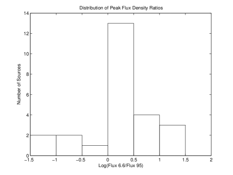
Figure 8: Comparison of the distribution of ratio of the 6.6-GHz peak flux density to the associated 95-GHz peak flux density for the twenty-five methanol masers in the statistically complete sample.

There are significant differences between the typical morphologies observed for class I and class II methanol masers. Class II methanol maser emission occurs in clusters with a maximum size of 30 milli-parsecs Caswell (1997); Phillips et al. (1998). The majority of sources have just one cluster, some have a second cluster separated by a few arcseconds, but more than two separate clusters in one region is very rare. In contrast the emission from class I masers is typically spread over much larger angular scales Kogan & Slysh (1998); Kurtz et al. (2004). This suggests enhanced methanol abundance over a significant fraction of the star formation region, but that conditions suitable for class II masers are relatively rare, while those that favour class I masers are more common.

Early interferometric observations of class I methanol masers suggested that they may be associated with outflows from high-mass star formation regions, perhaps at the interface between the outflow and the molecular cloud (Plambeck & Menten, 1990; Johnston et al., 1992). That they are observed offset from Hii regions, and are collisionally pumped is also consistent with this hypothesis. Further support has recently been provided by the observations of Kurtz et al. (2004) who found a number of sources for which there is a good correspondence between the 44 GHz class I masers and the molecular shock tracers H₂ and SiO.

It is well established that many water masers in star formation regions are associated with outflows, some of which have velocities in excess of 100 km/s and are highly collimated. Interferometric observations of water masers have shown that those with the largest peak flux densities lie in outflows directed at angles close to the plane of the sky (Genzel et al., 1981a, b). With this geometry our line-of-sight looks along the shock-front, giving a long velocity coherent path and hence strong masers. In contrast, masers which are significantly offset from the systemic velocity of the system are in outflows directed close to the line-of-sight, we view the shock-fronts close to face on resulting in short gain paths and weak masers.

The class I methanol masers are clearly not associated with the same outflows (or at least with the same parts of the outflows), as water masers, as they are always within 10-20 $\mbox{km~{}s}^{-1}$ of the velocity of class II masers and thermal emissions. However, we might expect class I methanol masers which are close to the systemic velocity of the region to be associated with outflows directed close to the plane of the sky and, analogous to water masers to be stronger. If we assume that the velocity of the class II masers is close to the systemic velocity of the region (which is generally the case), then we can test this hypothesis by comparing the flux density of class I masers which overlap the velocity range of the class II with those that don’t. Figure 9 shows two histograms which make this comparison. Only those class I methanol masers associated with class II masers in the statistically complete sample are included in Fig. 9. The two samples (18 sources which have overlap and 7 sources which don’t) are too small to allow definitive conclusions to be drawn. However, there may be a higher percentage of stronger class I methanol masers associated with sources where there is a velocity overlap between the two classes.

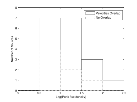
Figure 9: Comparison of the distribution of peak flux density for class I methanol masers which have a velocity range which overlaps the class II masers (solid line) and those which do not (dashed line). Only class I masers associated with class II masers in the statistically complete sample are included in this figure.

Two types of observations suggest that class II methanol masers are associated with the early stages of high-mass star formation.

1. Many class II methanol masers are not associated with an UCHii region (Phillips et al., 1998; Walsh et al., 1998).

2. Class II masers are associated with submillimetre and millimetre dust continuum emission which have SED consistent with deeply embedded high-mass protostellar objects Pestalozzi, Humphreys & Booth (2002); Walsh et al. (2003); Minier et al. (2004)

The current star formation paradigm for low-mass star formation has molecular outflows associated with the earliest stages of the process, the so-called class 0 and class I young stellar objects (Bachiller & Tafalla, 1999). From this we might hypothesise that class I methanol masers may be associated with an even earlier stage of high-mass star formation than is the general case for class II masers. Considering only methanol masers we might expect sources with only class I methanol masers to be the youngest, with those which have both class I and II masers being at an intermediate phase and sources with only class II methanol masers being the most evolved. We can test this hypothesis by looking at the properties of the infrared sources and other maser species associated with the methanol masers and seeing if there is any difference between the class II masers with and without an associated class I maser. If a difference can be found then it would also provide a method of targeting class I methanol maser searches.

The two most common masers associated with high-mass star formation (apart from class II methanol masers) are the 1665-MHz transition of OH and the 22-GHz transition of water. An untargeted search of the southern Galactic plane for main-line OH masers was made with the Parkes telescope in the early 1980s (Caswell et al., 1980; Caswell & Haynes, 1983a, 1987), with some regions more recently searched again at higher sensitivity with the Australia Telescope Compact Array (Caswell, 1998). The Parkes search was sensitive to OH masers with a peak flux density in excess of 1 Jy in the main-line transition at the epoch of the observations. To date there have been no blind searches for southern water masers. However, a search targeted towards the 6.6-GHz methanol masers detected in the Mt Pleasant survey has been undertaken by Hanslow (1997). Table 6 summarises the association of the class II methanol masers from the Mt Pleasant survey with 1665-MHz OH and 22-GHz water masers. Considering only the class II methanol masers in the statistically complete sample, approximately 30 percent have an associated 1665-MHz OH maser and approximately 40 percent have an associated water maser. However, there is no statistically significant correlation, or anti-correlation between the presence of OH or water masers and class I methanol masers.

Table 6: Associations of the class II methanol masers with other maser species and MSX 21-µm flux. The MSX flux is measured directly from the images, for non-detections the flux density at the maser location is given as an upper limit. Notes : ^a sources not within the statistically complete sample of 6.6-GHz methanol masers. References 1 = Caswell & Haynes (1987) ; 2 = Caswell (1998) ; 3 = Caswell & Haynes (1983b) ; 4 = Caswell et al. (1995b) ; 5 = Hanslow (1997)

Source	1665-MHz		22-GHz		MSX
Name	OH maser		$\mbox{H}_{2}\mbox{O}$ maser		21-µm flux
	Assoc	Ref	Assoc	Ref	($\mu$Wm-2sr-1)
$285.32\!-\!0.03$	N	1	Y	5	$<$1.25
$291.28\!-\!0.71$	N	1	Y	5	1600
$293.84\!-\!0.78$	N	1	Y	5	$<$0.15
$293.95\!-\!0.91$	N	1	Y	5	$<$0.77
$326.475\!+\!0.703$	N	2	Y	5	$<$0.87
$326.641\!+\!0.613^{a}$	N	2	Y	5	$<$12.5
$326.662\!+\!0.521$	N	2	Y	5	330
$326.859\!-\!0.677^{a}$	N	2	N	5	$<$3.6
$327.120\!+\!0.511$	Y	2	Y	5	71
$327.392\!+\!0.199$	N	2	N	5	9.6
$327.401\!+\!0.445$	N	2	N	5	55
$327.402\!+\!0.444$	Y	2	Y	5	41
$327.590\!-\!0.094$	N	2	N	5	9.5
$327.618\!-\!0.111$	N	2	N	5	8.1
$327.945\!-\!0.115$	N	2	N	5	57
$328.254\!-\!0.532$	Y	2	Y	5	53
$328.237\!-\!0.548^{a}$	Y	2	Y	5	7.6
$328.809\!+\!0.633^{a}$	Y	2	N	5	510
$329.031\!-\!0.198$	Y	2	Y	5	$<$4.0
$329.029\!-\!0.205$	Y	2	Y	5	$<$3.6
$329.066\!-\!0.308$	Y	2	N	5	20
$329.183\!-\!0.314$	Y	2	Y	5	$<$5.7
$329.339\!+\!0.148$	N	2	N	5	700
$329.407\!-\!0.459$	Y	2	Y	5	19
$329.469\!+\!0.502$	N	2	N	5	$<$4.7
$329.622\!+\!0.138$	N	2	Y	5	$<$0.53
$329.610\!+\!0.114$	N	2	N	5	27
$330.952\!-\!0.182^{a}$	Y	2	Y	5	130
$331.425\!+\!0.264^{a}$	N	2	N	5	$<$3.8
$331.120\!-\!0.118^{a}$	N	2		5	$<$3.1
$331.132\!-\!0.244$	Y	2	Y	5	21
$331.278\!-\!0.188$	Y	2	Y	5	95
$331.342\!-\!0.346$	Y	2	N	5	60
$331.442\!-\!0.187^{a}$	Y	2	Y	5	8.7
$331.542\!-\!0.066$	Y	2	N	5	320
$331.556\!-\!0.121^{a}$	Y	2	Y	5	106
$332.094\!-\!0.421$	N	2	Y	5	480
$332.295\!-\!0.094$	N	2	Y	5	71
$332.351\!-\!0.436$	N	2	N	5	$<$2.8
$332.560\!-\!0.148$	N	2	N	5	$<$11
$332.604\!-\!0.167$	N	2	N	5	$<$3.0
$332.942\!-\!0.686^{a}$	N	2	Y	5	$<$8.6
$332.963\!-\!0.679^{a}$	N	2	N	5	31
$333.029\!-\!0.015$	N	2	N	5	$<$4.8
$333.029\!-\!0.063^{a}$	N	2		5	32
$333.068\!-\!0.447$	N	2	N	5	120
$333.121\!-\!0.434$	N	2	Y	5	420
$333.128\!-\!0.440$	N	2	Y	5	420
$333.130\!-\!0.560^{a}$	N	2	Y	5	$<$7.1
$333.163\!-\!0.101^{a}$	N	2	N	5	58
$333.184\!-\!0.091$	N	2	N	5	$<$11
$333.234\!-\!0.062$	Y	2	Y	5	$<$6.0
$333.315\!+\!0.105$	Y	2	N	5	56
$333.466\!-\!0.164$	Y	2	Y	5	29
$333.562\!-\!0.025$	N	2	N	5	$<$3.9

Table 7: continued

Source	1665-MHz		22-GHz		MSX
Name	OH maser		$\mbox{H}_{2}\mbox{O}$ maser		21-µm flux
	Assoc	Ref	Assoc	Ref	($\mu$Wm-2sr-1)
$333.646\!+\!0.058^{a}$	N	2		5	$<$3.3
$333.683\!-\!0.437$	N	2	N	5	1.3
$333.931\!-\!0.135$	N	2	N	5	10.0
$334.635\!-\!0.015$	N	2	N	5	$<$1.9
$334.935\!-\!0.098^{a}$	N	2		5	$<$1.4
$335.060\!-\!0.427^{a}$	Y	2	Y	5	17
$25.386\!+\!0.005$	N	3	N	5	$<$4.4
$25.411\!+\!0.105$	N	3	N	5	28
$25.53+\!0\!.38$	N	3	N	5	$<$1.7
$25.710\!+\!0.044$	N	3	N	5	21
$25.826\!-\!0.178$	N	3	Y	5	$<$2.8
$26.528\!-\!0.266$	N	3	N	5	$<$7.4
$26.602\!-\!0.220$	N	3	N	5	$<$3.7
$27.223\!+\!0.137$	N	3	N	5	$<$7.4
$27.286\!+\!0.151^{a}$	N	3	N	5	9.3
$27.369\!-\!0.164$	Y	3	Y	5	11
$28.151\!-\!0.002$	N	3	N	5	$<$5.2
$28.201\!-\!0.049$	Y	3	N	5	230
$28.303\!-\!0.389$	N	3	N	5	120
$28.829\!+\!0.488$	N	3	Y	5	$<$1.8
$28.863\!-\!0.237$	Y	3	N	5	$<$3.6
$28.810\!+\!0.360$	N	3	Y	5	$<$1.7
$29.313\!-\!0.165$	N	3	N	5	$<$1.9
$29.867\!-\!0.042$	Y	4	N	5	13
$29.865\!-\!0.007$	N	3	N	5	$<$2.5
$29.895\!-\!0.047$	N	3	N	5	$<$11
$29.907\!-\!0.040$	N	3	N	5	14
$29.918\!-\!0.035$	Y	4	N	5	18
$29.923\!+\!0.059$	N	3	N	5	$<$0.35
$29.974\!-\!0.029$	N	3	Y	5	17
$30.009\!-\!0.017$	N	3	N	5	$<$4.7

4.1 Infrared characteristics of class I and II methanol masers

A number of searches for class II methanol masers have been targeted towards IRAS sources with far-infrared colours within certain ranges (e.g. Schutte et al., 1993; Walsh et al., 1997; Slysh et al., 1999; Szymczak et al., 2000). The current class I maser observations were targeted towards class II methanol maser positions, the vast majority of which are known to sub-arcsecond accuracy. So it is possible to reliably determine whether infrared sources from the IRAS, MSX and 2MASS point sources catalogues are associated with the maser positions. If the sources with class I methanol masers represent a different evolutionary phase from those without then this may lead to an observable difference in the properties of associated infrared sources. In this section we examine the characteristics of IRAS, MSX and 2MASS sources associated with the masers to see if there is any difference between those class II methanol masers with and without associated class I masers. Some readers may prefer to skip to the concluding paragraph of this section where the results are summerised, rather read all the details of the comparisons undertaken that are given below.

Considering only the statistically complete sample of sixty-eight class II methanol masers, 30 have an associated IRAS point source (IRAS Science Working Group, 1985) within 30 arcsec, 45 have an associated MSX point source (Egan et al., 2003) within 30 arcsec and 45 have an associated 2MASS source within 5 arcsec. The names and the distance between the infrared point source and maser positions are summarised in table 8.

There are 11 IRAS sources which exhibit both class I and II methanol maser emission (version 2.1 of the IRAS PSC). This is consistent with the number expected by chance considering the relative proportions of class II methanol maser sources with associated class I masers and IRAS sources. Examining a plot of the $F_{25}/F_{12}$ versus $F_{60}/F_{25}$ colours (where $F_{12},F_{25}$ and $F_{60}$ are the IRAS 12-, 25- and 60-µm flux densities respectively) there is no apparent difference between those IRAS sources with and without an associated class I methanol maser. So there doesn’t appear to be any means of using IRAS colours to select high-mass star forming regions that are more likely to have associated class I methanol masers, beyond the well known ultra-compact Hii region criteria developed by Wood & Churchwell (1989). This implies that any evolutionary difference between class II maser sources with and without associated class I masers cannot be distinguished from IRAS data.

Table 8: Associations of the class II methanol masers with IRAS, MSX and 2MASS point sources. Notes : ^a sources not within the statistically complete sample of 6.6-GHz methanol masers.

Source	IRAS		MSX		2MASS
Name	Name	Distance	Name	Distance	Name	Distance
		(arcsec)		(arcsec)		(arcsec)
$285.32\!-\!0.03$	$10303\!-\!5746$	21.4	G$285.3472\!+\!00.0013$	17.9	$10321294\!-\!5802306$	4.8
$291.28\!-\!0.71$	$11097\!-\!6102$	19.4	G$291.2731\!-\!00.7101$	16.0	$11115460\!-\!6118279$	2.7
$293.84\!-\!0.78$	$11298\!-\!6155$	1.3	G$293.8282\!-\!00.7445$	1.6	$11320631\!-\!6212206$	2.4
$293.95\!-\!0.91$	$11304\!-\!6206$	1.1	G$293.9512\!-\!00.8941$	6.4	$11324316\!-\!6223048$	2.2
$326.475\!+\!0.703$	$15394\!-\!5358$	20.8			$15431671\!-\!5407089$	3.8
$326.641\!+\!0.613^{a}$					$15443293\!-\!5405293$	0.8
$326.662\!+\!0.521$	$15412\!-\!5359$	6.9	G$326.6618\!+\!00.5207$	0.8	$15450281\!-\!5409030$	0.4
$326.859\!-\!0.677^{a}$
$327.120\!+\!0.511$	$15437\!-\!5343$	3.6	G$327.1192\!+\!00.5103$	1.9	$15473282\!-\!5352398$	1.2
$327.392\!+\!0.199$	$15464\!-\!5348$	4.0	G$327.3941\!+\!00.1970$	12.2	$15501855\!-\!5357087$	2.4
$327.401\!+\!0.445$			G$327.4014\!+\!00.4454$	3.4
$327.402\!+\!0.444$			G$327.4014\!+\!00.4454$	4.5	$15491950\!-\!5345096$	4.5
$327.590\!-\!0.094$					$15523652\!-\!5403157$	4.1
$327.618\!-\!0.111$			G$327.6184\!-\!00.1109$	0.4	$15525032\!-\!5402596$	1.3
$327.945\!-\!0.115$	$15507\!-\!5341$	2.8	G$327.9455\!-\!00.1149$	3.5	$15543391\!-\!5350446$	0.1
$328.254\!-\!0.532$	$15541\!-\!5349$	2.7	G$328.2523\!-\!00.5320$	5.9
$328.237\!-\!0.548^{a}$			G$328.2396\!-\!00.5460$	12.3
$328.809\!+\!0.633^{a}$	$15520\!-\!5234$	4.1	G$328.8074\!+\!00.6324$	4.7	$15554848\!-\!5243018$	4.5
$329.031\!-\!0.198$	$15566\!-\!5304$	8.4			$16003085\!-\!5312268$	4.8
$329.029\!-\!0.205$	$15566\!-\!5304$	17.6
$329.066\!-\!0.308$	$15573\!-\!5307$	2.2	G$329.0663\!-\!00.3081$	2.2	$16010999\!-\!5316029$	0.6
$329.183\!-\!0.314$	$15579\!-\!5303$	5.2
$329.339\!+\!0.148$	$15567\!-\!5236$	5.9	G$329.3371\!+\!00.1469$	7.7
$329.407\!-\!0.459$	$15596\!-\!5301$	13.1	G$329.4055\!-\!00.4574$	8.1
$329.469\!+\!0.502$			G$329.4626\!+\!00.5037$	23.2	$15594047\!-\!5223265$	2.6
$329.622\!+\!0.138$					$16020013\!-\!5233578$	2.0
$329.610\!+\!0.114$			G$329.6098\!+\!00.1139$	1.2	$16020313\!-\!5235328$	0.7
$330.952\!-\!0.182^{a}$			G$330.9544\!-\!00.1817$	6.8	$16095195\!-\!5154595$	4.2
$331.425\!+\!0.264^{a}$
$331.120\!-\!0.118^{a}$			G$331.1195\!-\!00.1191$	4.5
$331.132\!-\!0.244$	$16071\!-\!5142$	26.7	G$331.1282\!-\!00.2436$	12.8	$16105979\!-\!5150253$	2.7
$331.278\!-\!0.188$	$16076\!-\!5134$	10.4	G$331.2759\!-\!00.1891$	8.7
$331.342\!-\!0.346$			G$331.3402\!-\!00.3444$	8.5	$16122648\!-\!5146177$	0.9
$331.442\!-\!0.187^{a}$			G$331.4442\!-\!00.1877$	9.0
$331.542\!-\!0.066$			G$331.5414\!-\!00.0675$	5.1	$16120865\!-\!5125488$	3.6
$331.556\!-\!0.121^{a}$	$16086\!-\!5119$	26.6	G$331.5582\!-\!00.1206$	9.5	$16122682\!-\!5127389$	3.7
$332.094\!-\!0.421$	$16124\!-\!5110$	3.8	G$332.0939\!-\!00.4206$	1.3	$16161646\!-\!5118251$	0.3
$332.295\!-\!0.094$	$16119\!-\!5048$	8.1	G$332.2944\!-\!00.0962$	9.7	$16154514\!-\!5055511$	3.4
$332.351\!-\!0.436$	$16137\!-\!5100$	9.6			$16173117\!-\!5108181$	5.0
$332.560\!-\!0.148$			G$332.5555\!-\!00.1429$	23.5
$332.604\!-\!0.167$
$332.942\!-\!0.686^{a}$	$16175\!-\!5046$	23.0	G$332.9419\!-\!00.6849$	3.3
$332.963\!-\!0.679^{a}$	$16175\!-\!5045$	2.8	G$332.9636\!-\!00.6800$	4.3
$333.029\!-\!0.015$			G$333.0274\!-\!00.0131$	9.3	$16184404\!-\!5021487$	2.4
$333.029\!-\!0.063^{a}$			G$333.0299\!-\!00.0645$	7.1	$16185660\!-\!5023542$	1.2
$333.068\!-\!0.447$			G$333.0682\!-\!00.4461$	3.3
$333.121\!-\!0.434$			G$333.1256\!-\!00.4367$	20.2	$16205937\!-\!5035516$	3.2
$333.128\!-\!0.440$			G$333.1256\!-\!00.4367$	14.6	$16210349\!-\!5035505$	2.0
$333.130\!-\!0.560^{a}$					$16213571\!-\!5040527$	1.5
$333.163\!-\!0.101^{a}$	$16159\!-\!5012$	20.3	G$333.1642\!-\!00.0994$	5.6	$16194245\!-\!5019532$	2.0
$333.184\!-\!0.091$					$16194611\!-\!5018365$	5.0
$333.234\!-\!0.062$					$16195102\!-\!5015176$	4.1
$333.315\!+\!0.105$	$16157\!-\!4957$	2.9	G$333.3151\!+\!00.1053$	0.8	$16192910\!-\!5004432$	2.0
$333.466\!-\!0.164$	$16175\!-\!5002$	12.7	G$333.4680\!-\!00.1603$	16.1
$333.562\!-\!0.025$					$16210884\!-\!4959484$	0.5
$333.646\!+\!0.058^{a}$			G$333.6506\!+\!00.0598$	20.2	$16210963\!-\!4952455$	4.8
$333.683\!-\!0.437$	$16196\!-\!5005$	14.0	G$333.6788\!-\!00.4344$	15.5	$16232951\!-\!5012118$	4.1
$333.931\!-\!0.135$	$16194\!-\!4941$	25.0	G$333.9305\!-\!00.1319$	9.4
$334.635\!-\!0.015$	$16220\!-\!4906$	7.9	G$334.6340\!-\!00.0125$	8.6	$16254596\!-\!4913388$	2.6
$334.935\!-\!0.098^{a}$					$16272411\!-\!4904076$	3.9
$335.060\!-\!0.427^{a}$	$16256\!-\!4905$	17.6	G$335.0611\!-\!00.4261$	7.6	$16292288\!-\!4912259$	3.0

Table 9: continued

Source	IRAS		MSX		2MASS
Name	Name	Distance	Name	Distance	Name	Distance
		(arcsec)		(arcsec)		(arcsec)
$25.386\!+\!0.005$			G$025.3865\!+\!00.0036$	6.8
$25.411\!+\!0.105$	$18345\!-\!0641$	4.6	G$025.4118\!+\!00.1052$	3.0	$18371690\!-\!0638304$	2.2
$25.53+\!0\!.38$					$18363259\!-\!0624251$	0.9
$25.710\!+\!0.044$			G$025.7058\!+\!00.0403$	19.1
$25.826\!-\!0.178$					$18390338\!-\!0624096$	3.6
$26.528\!-\!0.266$			G$026.5254\!-\!00.2667$	9.6
$26.602\!-\!0.220$
$27.223\!+\!0.137$			G$027.2220\!+\!00.1361$	5.3	$18403043\!-\!0500569$	1.9
$27.286\!+\!0.151^{a}$					$18403448\!-\!0457137$	0.3
$27.369\!-\!0.164$	$18391\!-\!0504$	12.5	G$027.3652\!-\!00.1638$	12.1
$28.151\!-\!0.002$			G$028.1467\!-\!00.0040$	15.9
$28.201\!-\!0.049$	$18403\!-\!0417$	3.9	G$028.2007\!-\!00.0494$	0.7	$18425811\!-\!0413573$	1.4
$28.303\!-\!0.389$			G$028.3046\!-\!00.3871$	10.0	$18442217\!-\!0417463$	3.0
$28.829\!+\!0.488$					$18421219\!-\!0325376$	4.1
$28.863\!-\!0.237$
$28.810\!+\!0.360$
$29.313\!-\!0.165$	$18427\!-\!0320$	29.5			$18452474\!-\!0317411$	4.8
$29.867\!-\!0.042$			G$029.8620\!-\!00.0444$	20.7	$18455964\!-\!0244453$	2.6
$29.865\!-\!0.007$
$29.895\!-\!0.047$					$18460337\!-\!0243223$	4.9
$29.907\!-\!0.040$					$18460346\!-\!0242394$	3.6
$29.918\!-\!0.035$			G$029.9183\!-\!00.0404$	19.8
$29.923\!+\!0.059$					$18454403\!-\!0239052$	2.7
$29.974\!-\!0.029$			G$029.9738\!-\!00.0364$	28.2	$18460869\!-\!0238420$	2.9
$30.009\!-\!0.017$

The IRAS observations suffered well documented problems with confusion and saturation close to the Galactic Plane and this is thought to be the reason why many class II methanol maser sites have no associated IRAS source. Since if all class II methanol masers are associated with high-mass star formation (as argued the introduction) then they should show far-infrared emission, even those that are very young and enshrouded in cold dust. The MSX and 2MASS observations do not have the same problems as IRAS. However, they were made at shorter, mid- and near-infrared wavelengths. A total of 45 of the class II methanol maser sources in the statistically complete sample have an associated MSX source within 30 arcsec, and of these 14 also have an associated class I methanol maser. Version 2.3 of the MSX point source catalogue was used, which contains more than 25 percent more sources, and has greater photometric accuracy than earlier versions of the catalogue (Egan et al., 2003). If the sources with class I masers represent an earlier evolutionary phase then we would expect them to be more deeply embedded, and likely to show a lower rate of detection in the mid-infrared MSX observations. However, the proportion of class I methanol maser sources with an associated MSX source is within the range expected given the rate of association with the parent sample. Lumsden et al. (2002) investigated the MSX colours of a sample of massive young stellar objects (MYSO) and found that they show $F_{8}<F_{12}<F_{21}$ (where $F_{8}$, $F_{12}$ and $F_{21}$ are the MSX 8-, 12- and 21-µm flux densities respectively) and $F_{21}/F_{8}>2$. Figure 10 shows an MSX colour-colour plot of $F_{14}/F_{12}$ versus $F_{21}/F_{8}$ for the class II methanol maser sources with and without associated class I methanol masers, and included for comparison are all MSX sources within 30 arcsec of $l=326^{\circ}$, $b=0^{\circ}$. The majority of the maser sources meet the Lumsden et al. (2002) criteria for MYSO, that is they lie within the top right section of Fig 10. This is not particularly surprising as 6.6-GHz methanol masers without associated radio continuum emission from Walsh et al. (1998) were part of the sample of sources used to define the criteria. However, that a statistically complete sample of class II methanol masers shows the same characteristics in an MSX colour-colour plot as the IRAS-selected sample of Walsh et al. adds further weight to the widely accepted argument that the new class II methanol masers discovered in untargeted searches are in fact associated with high-mass star formation. The further towards the top-right of Fig 10 a source lies, the cooler the implied dust temperature, so we would expect younger, more deeply embedded sources to lie in this region. The class II methanol masers with and without associated class I masers show the same distribution, again suggesting that there is no significant evolutionary difference between the two groups.

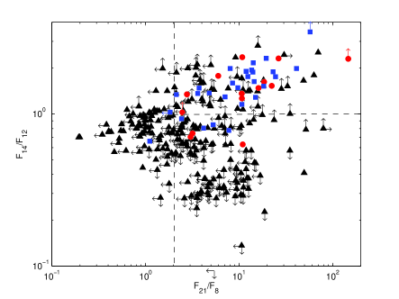
Figure 10: MSX colours $F_{14}/F_{12}$ versus $F_{21}/F_{8}$ for class II methanol masers with (circles) and without (squares) associated class I masers. The triangles are MSX sources within 30 arcsec of $l=326^{\circ}$, $b=0^{\circ}$. Sources with an upper limit in one of the MSX bands making up the ratio are marked with an arrow pointing in the appropriate direction. Sources with an upper limit in both MSX bands for either of the colours have been excluded from the plot. Sources within region within the dashed lines at the top right of the plot meet the MYSO criteria of Lumsden et al. (2002).

The quoted astrometric accuracy of the MSX point source catalogue is better than 2 arcsec (Egan et al., 2003). However, only 8 of the 45 MSX sources are within 2 arcsec of the class II maser position. In total 14 of the class II maser positions are within 5 arcsec and 29 are within 10 arcsec of an MSX point source. This suggests that in general the masers are offset from the MSX point sources, and probably associated with other objects within the larger star formation complex. It suggests that in many cases the colours of the MSX sources in Fig. 10 are not those of the source exciting the methanol masers and so will confuse any attempt to find differences between the class II masers with and without associated class I masers. However, it still may be possible to find such differences directly from the MSX image data. I have examined the 21-µm MSX (E-band) images in the vicinity of each of the maser sources and the results are summarise in Table 6. If the class I masers are associated with a generally earlier evolutionary phase, then we would expect a lower percentage to be projected against 21-µm emission. Considering the sixty-eight class II masers in the complete sample, thirty-five are projected against 21-µm emission, 15 of 26 with class I masers and 21 of 42 without. So approximately 50 percent of class II methanol maser sources are projected against 21-µm MSX emission, but there is no correlation with the presence or absence of associated class I masers. Of those maser sources that are not projected against 21-µm emission, some are near a source, but the majority are not. In contrast, for an IRAS-selected sample of nearly 50 UCHii regions, only one did not have coincident 21-µm MSX emission (Crowther & Conti, 2003).

Near-infrared observations of methanol maser sources are generally of limited use as most sources are thought to be optically thick at these wavelengths. However, for completeness the association of the methanol masers with sources in the 2MASS point source catalogue has been examined. Considering the statistically complete sample of sixty-eight sources, forty-five have a 2MASS point source within 5 arcsec, dropping to 13 within 2 arcsec. The proportion of these sources which also have an associated class I methanol maser matches the proportions for the sample as a whole. As for the MSX sources, it is likely that in many cases the 2MASS point sources are not directly associated with the masers, but rather a nearby source within the same region.

The association of the class II methanol masers in the statistically complete sample with IRAS, MSX and 2MASS sources has been investigated. There is no measurable difference, either in terms of rates of association, or the infrared colours between those class II masers with an associated class I maser and those without. Combining this with the similar finding for the association of other maser species, it suggests that class I methanol masers, like class II, are associated with star formation regions for a moderately long evolutionary period. For example $329.031\!-\!0.198$ is optically thick at a wavelength of 21-µm, suggesting it is deeply embedded and at an early evolutionary phase. In contrast $328.809\!+0\!.633$ has a well developed Hii region with some extended emission (Ellingsen, Shabala & Kurtz, 2005) and shows emission in a number of the rarer excited OH and class II maser transitions (Ellingsen et al., 2004, and references therein), which are believed to be associated with more evolved regions. The lack of any distinguishing characteristics between the class II masers with and without associated class I masers is consistent with the general assumption that the two classes of methanol maser are not directly associated. High-mass stars form in clusters and so it is likely that at any one time there are stars at a variety of evolutionary phases within the one region. If in general the star exciting the class II methanol masers is not the source of the outflow producing the class I masers then we would not expect any clear evolutionary relationship to be manifest. However, there are many other possible complicating factors, for example there is no reason to expect both classes of methanol maser to be associated with exactly the same stellar mass range. This complexity further highlights the general need for high-resolution observations to disentangle a high-mass star formation complex.

5 Conclusions

Class I methanol masers are associated with approximately half of all class II methanol maser sources. In contrast to previous suggestions, there is no anti-correlation between the velocity range of the two maser classes, nor their peak flux densities. The velocity ranges overlap in the majority of sources and there is some evidence that in those sources where there is an overlap the peak flux density of the class I masers is stronger. The peak flux density of the 6.6- and 95.1-GHz transitions in most sources is of the same order of magnitude. This suggests that the peak maser flux density in both transitions may be heavily influenced by a common factor, such as the general methanol abundance within the larger star formation region.

Interferometric observations of the class I masers are required to allow a more detailed examination of the relationship between the two methanol maser classes and their role in the larger high-mass star formation picture. In particular to determine if the overlap in the velocity ranges seen in many sources is associated with coincident or near-coincident emission from the two transitions, or is merely an artefact of turbulent velocity fields.

Investigation of other maser species and infrared sources associated with the methanol masers did not find any statistically significant correlations that can be used to target future class I maser searches. The absence of such correlations is consistent with the hypothesis that the objects responsible for producing class I methanol masers are in general not those that produce main-line OH, water or class II methanol masers, although there are other possible explanations.

References

- Bachiller & Tafalla (1999) Bachiller R., Tafalla M., 1999, in NATO Science series C540, The Origin of Stars and Planetary Systems, ed. C. J. Lada & N. D. Kylafis, 227
- Batrla & Menten (1988) Batrla W., Menten K. M., 1988, ApJ, 329, 117
- Batrla et al. (1987) Batrla W., Matthews H. E., Menten K. M., Walmsley C. M., 1987, Nat, 326, 49
- Caswell (1996) Caswell J. L., 1996, MNRAS, 279, 79
- Caswell (1997) Caswell J. L., 1997, MNRAS, 289, 203
- Caswell (1998) Caswell J. L., 1998, MNRAS, 297, 215
- Caswell & Haynes (1983a) Caswell J. L., Haynes R. F., 1983a, Aust. J Phys., 36, 361
- Caswell & Haynes (1983b) Caswell J. L., Haynes R. F., 1983b, Aust. J Phys., 36, 417
- Caswell et al. (1980) Caswell J. L., Haynes R. F., Goss W. M., 1980, Aust. J Phys., 33, 639
- Caswell & Haynes (1987) Caswell J. L., Haynes R. F., 1987, Aust. J Phys., 40, 215
- Caswell et al. (1995a) Caswell J. L., Vaile R. A., Ellingsen S. P., 1995, PASA, 12, 37
- Caswell et al. (1995b) Caswell J. L., Vaile R. A., Ellingsen S. P., Whiteoak J. B., Norris R. P., 1995, MNRAS, 272, 96
- Cragg et al. (1992) Cragg D. M., Johns K. P., Godfrey P. D., Brown R. D., 1992, MNRAS, 259, 203
- Crowther & Conti (2003) Crowther P. A., Conti P. S., 2003, MNRAS, 343, 143
- De Lucia et al. (1989) De Lucia F. C., Herbst E., Anderson T., Helminger, P., 1989, J. Mol. Spectrosc., 134, 395
- Egan et al. (2003) Egan M. P., Price S. D., Kraemer K. E., Mizuno D. R., Carey S. J., Wright C. O., Engelke C.W., Cohen M., Gugliotti G. M., 2003, The Midcourse Space Experiment Point Source Catalog Version 2.3 Explanatory Guide (AFRL-VS-TR-2003-1589). Natl. Tech. Inf. Serv, Springfield, VA.
- Ellingsen (1996) Ellingsen S. P., 1996, PhD thesis, University of Tasmania
- Ellingsen et al. (1996) Ellingsen S. P., von Bibra M. L., McCulloch P. M., Norris R. P., Deshpande A. A., Phillips C. J., 1996, MNRAS, 280, 378
- Ellingsen et al. (2004) Ellingsen S. P., Cragg D. M., Lovell J. E. J., Sobolev A. M., Ramsdale P. D., Godfrey P. D., 2004, MNRAS, 354, 401
- Ellingsen et al. (2005) Ellingsen S. P., Shabala S. S., Kurtz S. E., 2005, MNRAS, in press
- Genzel et al. (1981a) Genzel R., Reid M. J., Moran J. M., Downes D., 1981, ApJ, 244, 884
- Genzel et al. (1981b) Genzel R., Downes D., Schneps M. H., Reid M. J., Moran J. M., Kogan L. R., Kostenko V. I., Matveenko L. I., Ronnang B., 1981, ApJ 247, 1039
- IRAS Science Working Group (1985) IRAS Point Source Catalog, 1985, IRAS Science Working Group, U.S. Government Printing Office, Washington DC
- Hanslow (1997) Hanslow L. A., 1997, Honours thesis, University of Tasmania
- Houghton & Whiteoak (1995) Houghton S., Whiteoak J. B., 1995, MNRAS, 273, 1033
- Johnston et al. (1992) Johnston K. J., Gaume R., Stolovy, S., Wilson T. L., Walmsley C. M., Menten K. M., 1992, ApJ, 385, 232
- Kogan & Slysh (1998) Kogan L., Slysh V., 1998, ApJ, 497, 800
- Kurtz et al. (2004) Kurtz S., Hofner P., Álvarez C. V., 2004, ApJSS, 155, 149
- Kutner & Ulich (1981) Kutner M. L., Ulich B. L., 1981, ApJ, 250, 341
- Ladd et al. (2004) Ladd N., Phillips C., Purcell C., Kesteven M., 2004, CSIRO Memo “Specification of Freqeuncy and Velocity Scales for Mopra Spectra”
- Lumsden et al. (2002) Lumsden S. L., Hoare M. G., Oudmaijer R. D., Richards D., 2002, MNRAS, 336, 621
- Mehringer & Menten (1997) Mehringer D. M., Menten K. M., 1997, ApJ, 474, 346
- Menten (1991a) Menten K. M., 1991a, in ASP Conf. Ser. 16, Atoms, ions and molecules: New results in spectral line astrophysics, ed. A. D. Haschick & P. T. P. Ho, 119
- Menten (1991b) Menten K. M., 1991b, ApJ, 380, L75
- Minier et al. (2004) Minier V., Burton M. G., Hill T., Pestalozzi M. R., Purcell C., Garay G., Walsh A., Longmore S., 2004, A&A, in press
- Morimoto et al. (1985) Morimoto M., Ohishi M., Kanzawa T., 1985, ApJ, 288, L11
- Müller et al. (2004) Müller H. S. P., Menten K. M., Mäder H., 2004, A&A, 428, 1019
- Peng & Whiteoak (1992) Peng R. S., Whiteoak J. B., 1992, MNRAS, 254, 301
- Pestalozzi et al. (2002) Pestalozzi M., Humphreys E. M. L., Booth R. S., 2002, A&A, 384, L15
- Pestalozzi et al. (2004) Pestalozzi M., Minier V., Booth R., 2004, A&A, in press
- Phillips et al. (1998) Phillips C. J., Norris R. P., Ellingsen S. P., McCulloch P. M., 1998, MNRAS, 300, 1131
- Plambeck & Menten (1990) Plambeck R. L., Menten K. M., 1990, ApJ, 364, 555
- Plambeck & Wright (1988) Plambeck R. L., Wright M. C. H., 1988, ApJ, 330, L61
- Schutte et al. (1993) Schutte A. J., van der Walt D. J., Gaylard M. J., MacLeod G. C., 1993, 261, 783
- Szymczak et al. (2000) Szymczak M., Hrynek G., Kus A. J., 2000, A&AS, 143, 269
- Szymczak et al. (2002) Szymczak M., Kus A. J., Hrynek G., Kepa, A., Pazderski, E., 2002, A&A, 392, 277
- Slysh et al. (1994) Slysh V. I., Kalenskii S. V., Val’tts I. E., Otrupcek R., 1994, MNRAS, 268, 464
- Slysh et al. (1999) Slysh V. I., Val’tts I. E., Kalenskii S. V., Voronkov M. A., Palagi F., Tofani G., Catarzi M., 1999, A&AS, 134, 115
- Sobolev & Deguchi (1994) Sobolev A.M., Deguchi S., 1994, A&A, 291, 569
- Sobolev et al. ( 1997) Sobolev A. M., Cragg D. M., Godfrey P. D., 1997, MNRAS, 288, L39
- Val’tts et al. (2000) Val’tts, I. E., Ellingsen, S. P., Slysh, V. I., Kalenskii, S. V., Otrupcek R., Larinov G. M., 2000, MNRAS, 317, 315
- van der Walt et al. (1995) van der Walt D. J., Gaylard M. J., MacLeod G. C., 1995, A&ASS, 110, 81
- Voronkov et al. (2004) Voronkov M. A., Sobolev A. M., Ellingsen S. P., Ostrovskii A. B., 2004, MNRAS submitted
- Walsh et al. (1997) Walsh A. J., Hyland A. R., Robinson G., Burton M. G., 1997, MNRAS, 291, 261
- Walsh et al. (1998) Walsh A. J., Burton M. G., Hyland A. R., Robinson G., 1998, MNRAS, 301, 640
- Walsh et al. (2003) Walsh A. J., Macdonald G. H., Alvey N. D. S., Burton M. G., Lee J. -K., 2003, A&A, 410, 597
- Wiesemeyer et al. (2004) Wiesemeyer H., Thum C., Walmsley C. M., 2004, 428, 479
- Wilson et al. (1984) Wilson T. L., Walmsley C. M., Snyder L. E., Jewell P. R., 1984, A&A, 134, L7
- Wilson et al. (1985) Wilson T. L., Walmsley C. M., Menten K. M. Hermsen, W., 1985, A&A, 147, L19
- Wood & Churchwell (1989) Wood D. O. S., Churchwell E., 1989a, ApJ, 340, 265