Properties of detached shells around carbon stars

The nature of the mechanism responsible for producing the spectacular, geometrically thin, spherical shells found around some carbon stars has been an enigma for some time. Based on extensive radiative transfer modelling of both CO line emission and dust continuum radiation for all objects with known detached molecular shells, we present compelling evidence that these shells show clear signs of interaction with a surrounding medium. The derived masses of the shells increase with radial distance from the central star while their velocities decrease. A simple model for interacting winds indicate that the mass-loss rate producing the faster moving wind has to be almost two orders of magnitudes higher ($\sim$ 10^-5 M_⊙ yr^-1) than the slower AGB wind (a few 10^-7 M_⊙ yr^-1) preceding this violent event. At the same time, the present-day mass-loss rates are very low indicating that the epoch of high mass-loss rate was relatively short, on the order of a few hundred years. This, together with the number of sources exhibiting this phenomenon, suggests a connection with He-shell flashes (thermal pulses). We report the detection of a detached molecular shell around the carbon star DR~Ser, as revealed from new single-dish CO (sub-)millimetre line observations. The properties of the shell are similar to those characterising the young shell around U~Cam.

1 Introduction

The late evolutionary stages of low- to intermediate-mass stars, as they ascend the asymptotic giant branch (AGB), are characterized by the ejection of gas and dust via a slow (5 $-$ 30 km s^-1) stellar wind. This mass loss (on the order of $10^{-7}$ – $10^{-5}$ M_⊙ yr^-1) is crucial to the evolution of the star and a key process for enriching and replenishing the interstellar medium (e.g., Schröder et al. 1999; Schröder & Sedlmayr 2001). Yet, the mechanisms by which it occurs are not understood in detail. In particular, there is evidence that strong variations in the mass-loss rate, perhaps related to flashes of helium shell burning (Olofsson et al. 1990), can lead to the formation of circumstellar detached shells. The existence of such shells can be inferred from their excess emission at far-infrared wavelengths (due to a lack of hot dust close to the star, Willems & de Jong 1988; Zijlstra et al. 1992), and are confirmed by a ring-like morphology in maps of dust or CO line emission (e.g., Waters et al. 1994; Olofsson et al. 1996; Lindqvist et al. 1999; Olofsson et al. 2000).

Detached CO shells have been observed around about a half-dozen AGB stars (see review by Wallerstein & Knapp 1998), all of them carbon stars. However, only U~Cam (Lindqvist et al. 1996, 1999), TT~Cyg (Olofsson et al. 2000), and S~Sct (Olofsson et al., in prep.) have been mapped in detail with millimetre-wave interferometers. These three cases reveal remarkably symmetric shells expanding away from the stars. However, there are also clear indications of a highly clumped medium. High-resolution molecular line observations offer the possibility not only to confirm detachment, but also to study variations in mass loss on short ($<$100 yr) timescales, related to the shell thickness, and to look for departures from spherical symmetry. Single-dish CO maps provide evidence for detached CO shells also in the cases of R~Scl, U~Ant, and V644~Sco (Olofsson et al. 1996).

González Delgado et al. (2001, 2003) have imaged the circumstellar media of R~Scl and U~Ant in circumstellar scattered stellar light. They found evidence for both dust- and gas-scattered light in detached shells of sizes comparable to those found in the CO line emission. These data provide high-angular-resolution information, but the separation of dust- and gas-scattered light is problematic.

Based on colour-colour diagrams for a large sample of OH/IR stars Lewis et al. (2004) have recently suggested that the vast majority of them could have detached shells, possibly linked to a brief period of intense mass loss for oxygen-rich AGB stars (Lewis 2002). However, no detached CO shell has been found for any oxygen-rich object yet.

Evidence of detached dust shells have been found in the cases of U~Ant (Izumiura et al. 1997), U~Hya (Waters et al. 1994), Y~CVn (Izumiura et al. 1996), and R~Hya (Hashimoto et al. 1998). All, but the last are carbon stars. Except for U~Ant, there has been no detections of detached CO shells for these stars.

Olofsson et al. (1990) suggested that the detached shells were an effect of a mass-loss-rate modulation caused by a He-shell flash (i.e., a thermal pulse). Vassiliadis & Wood (1993) studied this in some more detail, and followed the total mass-loss history of an AGB star. More recently, Schröder et al. (1998), Schröder et al. (1999) and Wachter et al. (2002) combined stellar evolutionary models and mass-loss prescriptions to study the effects on the evolution of an AGB star. They argued that during the low-mass-loss-rate evolution only carbon stars reach a critical (Eddington-like) luminosity that drives an intense mass ejection during a He-shell flash, hence explaining the absence (or at least rare occurrence) of detached shells towards M-type AGB stars. At higher mass-loss rates the detached shells become, in comparison, less conspicuous. Steffen & Schönberner (2000) used hydrodynamical simulations to follow the circumstellar evolution due to changes in the stellar mass-loss rate. They verified that a brief period of very high mass-loss rate translates into an expanding, geometrically thin shell around the star. They also concluded that an interacting-wind scenario is an equally viable explanation for the detached shells.

Less dramatic modulations of the mass-loss rate on shorter time scales have been observed towards the archetypical high-mass-loss-rate carbon star IRC+10216 (Mauron & Huggins 1999, 2000; Fong et al. 2003). Thin arcs, produced by mass-loss-rate modulations while the central star was ascending the AGB, are also seen around PPNe (Hrivnak et al. 2001; Su et al. 2003) and PNe (Corradi et al. 2004).

In this paper we present new single-dish millimetre line observations of R~Scl, U~Cam, V644~Sco, and DR~Ser, Sect. 2. Of particular importance is the detection of a new carbon star with a young detached molecular shell, DR~Ser, increasing the number of such stars to seven. In fact, there is not much hope of increasing this number further since most of the reasonably nearby AGB stars with mass loss have already been searched for circumstellar CO radio line emission. Section 3 describes the analysis of the molecular line and dust emission. Properties of the detached shells (Sect. 4), and the present-day winds (Sect. 5) of seven carbon stars with detached molecular shells, Table 1, are estimated. The results are discussed in Sect. 6, where different scenarios for producing the shells are reviewed. The usefulness of future high spatial resolution, as well as high-$J$ CO observations, in further constraining the shell characteristics are also discussed. Our conclusions are presented in Sect. 7.

Table 1: Carbon stars with detached molecular shells.

$$\begin{array}[]{p{0.3\linewidth}lclccl}\hline\cr\vskip 3.0pt plus 1.0pt minus 1.0pt\cr\lx@intercol{\mathrm{Source}}\hfil\lx@intercol&\lx@intercol\hfil{\mathrm{RA}}(2000.0)\hfil\lx@intercol&&\lx@intercol\hfil{\mathrm{DEC}}(2000.0)\hfil\lx@intercol&&\lx@intercol\hfil{\mathrm{Ref.}}\hfil\lx@intercol\\ &\lx@intercol\hfil[\mathrm{h:m:s}]\hfil\lx@intercol&&\lx@intercol\hfil[{\degr:\arcmin:\arcsec}]\hfil\lx@intercol&&\\ \vskip 3.0pt plus 1.0pt minus 1.0pt\cr\hline\cr\vskip 3.0pt plus 1.0pt minus 1.0pt\cr R Scl&\mbox{01:26:58.09}&&-\mbox{32:32:35.5}&&1\\ U Cam&\mbox{03:41:48.17}&&\phantom{-}\mbox{62:38:54.5}&&2\\ U Ant&\mbox{10:35:12.85}&&-\mbox{39:33:45.3}&&3\\ V644 Sco&\mbox{17:26:18.7}&&-\mbox{40:01:52}&&4\\ DR Ser&\mbox{18:47:21.02}&&\phantom{-}\mbox{05:27:18.6}&&3\\ S Sct&\mbox{18:50:20.04}&&-\mbox{07:54:27.4}&&3\\ TT Cyg&\mbox{19:40:57.00}&&\phantom{-}\mbox{32:37:05.9}&&5\\ \vskip 3.0pt plus 1.0pt minus 1.0pt\cr\hline\cr\end{array}$$

Refs. – 1) Wong et al. (2004), 2) Lindqvist et al. (1999), 3) Hipparcos catalogue, 4) Kholopov et al. (1985), 5) Olofsson et al. (2000).

2 Observations

2.1 Molecular line observations

Olofsson et al. (1996) published molecular line spectra obtained towards all the stars in Table 1, but U~Cam and DR~Ser. Additional (sub)millimetre single-dish spectra used in the present analysis have been published in Olofsson et al. (1993a, b), Schöier & Olofsson (2001), and Wong et al. (2004).

In this paper we present some complementary observational data. The James Clerk Maxwell Telescope (JCMT) located at Mauna Kea was used to collect CO $J=3\rightarrow 2$ (345.796 GHz) and $J=4\rightarrow 3$ (461.041 GHz) line emission from R~Scl, DR~Ser, and U~Cam. The observations were performed in June, July, and October 2003, except for the $J=4\rightarrow 3$ observations towards U~Cam which were done in November 2000. CO $J=1\rightarrow 0$ (115.271 GHz) and $J=2\rightarrow 1$ (230.538 GHz) line emission from U~Cam was obtained in November 1999 using the IRAM 30 m telescope at Pico Veleta. In addition, CO $J=1\rightarrow 0$ line emission towards TT Cyg and ¹³CO $J=2\rightarrow 1$ (220.399 GHz) line emission towards V644~Sco were detected using SEST in April 2002. The HCN $J=1\rightarrow 0$ (88.632 GHz) data for DR~Ser were collected during 1996-1997 using the Onsala Space Observatory (OSO) 20 m telescope. HCN $J=1\rightarrow 0$ and $J=3\rightarrow 2$ (265.886 GHz) observations of V644~Sco were obtained using the Swedish-ESO submillimetre telescope (SEST) at La Silla in April 2002.

Table 2: Summary of single-dish millimetre line observations used in the analysis.

$$\begin{array}[]{p{0.25\linewidth}llcc}\hline\cr\vskip 3.0pt plus 1.0pt minus 1.0pt\cr\lx@intercol{\mathrm{Source}}\hfil\lx@intercol&\lx@intercol\hfil{\mathrm{Telescope}}\hfil\lx@intercol&\lx@intercol\hfil{\mathrm{Transition}}\hfil\lx@intercol&\lx@intercol\hfil\int T_{\mathrm{mb}}\mathrm{d}v\hfil\lx@intercol&\lx@intercol\hfil{\mathrm{Ref.}}\hfil\lx@intercol\\ &&&\lx@intercol\hfil\mathrm{[K\,km\,s}^{-1}]\hfil\lx@intercol\\ \vskip 3.0pt plus 1.0pt minus 1.0pt\cr\hline\cr\vskip 3.0pt plus 1.0pt minus 1.0pt\cr R Scl&\mathrm{IRAM}&\mathrm{CO(1-0)}&76.2&4\\ &\mathrm{IRAM}&\mathrm{CO(2-1)}&67.7&4\\ &\mathrm{SEST}&\mathrm{CO(1-0)}&26.1&4\\ &\mathrm{SEST}&\mathrm{CO(2-1)}&47.8&4\\ &\mathrm{SEST}&\mathrm{CO(3-2)}&63.7&3\\ &\mathrm{JCMT}&\mathrm{CO(2-1)}&50.6&6\\ &\mathrm{JCMT}&\mathrm{CO(3-2)}&62.8&1\\ &\mathrm{JCMT}&\mathrm{CO(4-3)}&63.2&1\\ &\mathrm{SEST}&{}^{13}\mathrm{CO(1-0)}&\phantom{0}1.9&5\\ &\mathrm{SEST}&{}^{13}\mathrm{CO(2-1)}&\phantom{0}4.2&5\\ &\mathrm{SEST}&\mathrm{HCN(1-0)}&\phantom{0}1.3&3\\ &\mathrm{SEST}&\mathrm{HCN(3-2)}&\phantom{0}7.7&3\\ &\mathrm{SEST}&\mathrm{HCN(4-3)}&\phantom{0}3.9&3\\ &\mathrm{HHT}&\mathrm{HCN(3-2)}&\phantom{0}2.4&7\\ &\mathrm{HHT}&\mathrm{HCN(4-3)}&\phantom{0}4.1&7\\ U Cam&\mathrm{IRAM}&\mathrm{CO(1-0)}&21.8&1\\ &\mathrm{IRAM}&\mathrm{CO(2-1)}&97.9&1\\ &\mathrm{JCMT}&\mathrm{CO(3-2)}&66.7&1\\ &\mathrm{JCMT}&\mathrm{CO(4-3)}&54.6&1\\ U Ant&\mathrm{SEST}&\mathrm{CO(1-0)}&10.8&3\\ &\mathrm{SEST}&\mathrm{CO(2-1)}&13.1&3\\ &\mathrm{SEST}&\mathrm{CO(3-2)}&\phantom{0}9.7&3\\ V644 Sco&\mathrm{SEST}&\mathrm{CO(1-0)}&\phantom{0}7.6&3\\ &\mathrm{SEST}&\mathrm{CO(2-1)}&20.7&3\\ &\mathrm{SEST}&\mathrm{CO(3-2)}&21.4&3\\ &\mathrm{JCMT}&\mathrm{CO(2-1)}&22.2&6\\ &\mathrm{JCMT}&{}^{13}\mathrm{CO(2-1)}&\phantom{0}1.1&1\\ &\mathrm{SEST}&\mathrm{HCN(1-0)}&\phantom{0}0.3&1\\ &\mathrm{SEST}&\mathrm{HCN(3-2)}&\phantom{0}0.4&1\\ DR Ser&\mathrm{SEST}&\mathrm{CO(1-0)}&\phantom{0}3.7&2\\ &\mathrm{NRAO}&\mathrm{CO(2-1)}&11.3&2\\ &\mathrm{JCMT}&\mathrm{CO(3-2)}&14.7&1\\ &\mathrm{JCMT}&\mathrm{CO(4-3)}&\phantom{0}8.5&1\\ &\mathrm{OSO}&\mathrm{HCN(1-0)}&\phantom{0}0.6&1\\ S Sct&\mathrm{SEST}&\mathrm{CO(1-0)}&\phantom{0}5.8&3\\ &\mathrm{SEST}&\mathrm{CO(2-1)}&\phantom{0}4.3&3\\ &\mathrm{SEST}&\mathrm{CO(3-2)}&\phantom{0}3.1&3\\ &\mathrm{SEST}&{}^{13}\mathrm{CO(1-0)}&\phantom{0}0.2&3\\ TT Cyg&\mathrm{SEST}&\mathrm{CO(1-0)}&\phantom{0}5.0&1\\ &\mathrm{OSO}&\mathrm{CO(1-0)}&\phantom{0}6.4&3\\ &\mathrm{IRAM}&\mathrm{CO(1-0)}&\phantom{0}7.5&3\\ &\mathrm{IRAM}&\mathrm{CO(2-1)}&\phantom{0}6.0&3\\ \vskip 3.0pt plus 1.0pt minus 1.0pt\cr\hline\cr\end{array}$$

Refs. – 1) This paper. 2) Schöier & Olofsson (2001). 3) Olofsson et al. (1996). 4) Olofsson et al. (1993b). 5) Schöier & Olofsson (2000). 6) JCMT public archive. 7) Bieging (2001).

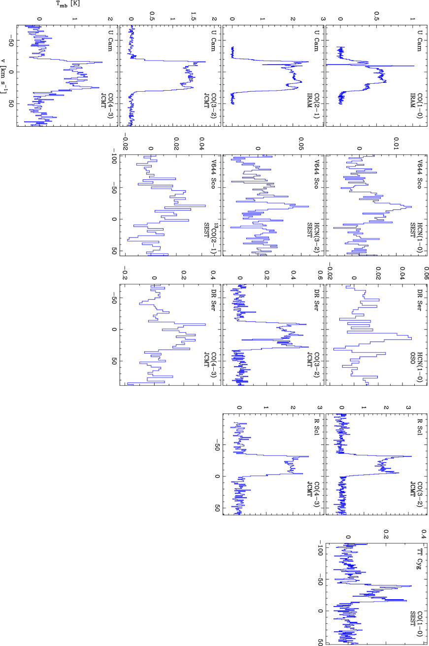
Figure 1: New observations of CO and HCN radio line emission.

All observations were made in a dual beamswitch mode, where the source is alternately placed in the signal and the reference beam, using a beam throw of about $2\arcmin$ at JCMT, $4\arcmin$ at IRAM, $11\arcmin$ at OSO, and $12\arcmin$ at SEST. This method produces very flat baselines. Regular pointing checks made on strong continuum sources (JCMT and IRAM) or SiO masers (OSO and SEST) were found to be consistent within $\approx$ 3$\arcsec$.

The observed spectra are presented in Fig. 1 and velocity-integrated intensities are reported in Table 2. The intensity scales are given in main beam brightness temperature, $T_{\mathrm{mb}}$ = $T_{\mathrm{A}}^{*}/\eta_{\mathrm{mb}}$, where $T_{\mathrm{A}}^{\star}$ is the antenna temperature corrected for atmospheric attenuation using the chopper wheel method, and $\eta_{\mathrm{mb}}$ is the main beam efficiency. For the CO $J=3\rightarrow 2$ and $J=4\rightarrow 3$ observations at the JCMT we have used main-beam efficiencies of 0.62 and 0.5, respectively. For the IRAM CO $J=1\rightarrow 0$ and $J=2\rightarrow 1$ observations we have used main-beam efficiencies ($B_{\mathrm{eff}}/F_{\mathrm{eff}}$) of 0.7 and 0.5, respectively. For the HCN $J=1\rightarrow 0$ data obtained at OSO $\eta_{\mathrm{mb}}=0.65$ was used. For the SEST $\eta_{\mathrm{mb}}=0.75$ was used for the HCN $J=1\rightarrow 0$ data, $\eta_{\mathrm{mb}}=0.7$ for the CO $J=1\rightarrow 0$ data, and $\eta_{\mathrm{mb}}=0.5$ for the HCN $J=3\rightarrow 2$ and ¹³CO $J=2\rightarrow 1$ observations. The uncertainty in the absolute intensity scale is estimated to be about $\pm 20$%.

The data was reduced in a standard way, by removing a first order baseline and then binned in order to improve the signal-to-noise ratio, using XS.

A summary of the available data, relevant to the analysis in this paper, are given in Table 2.

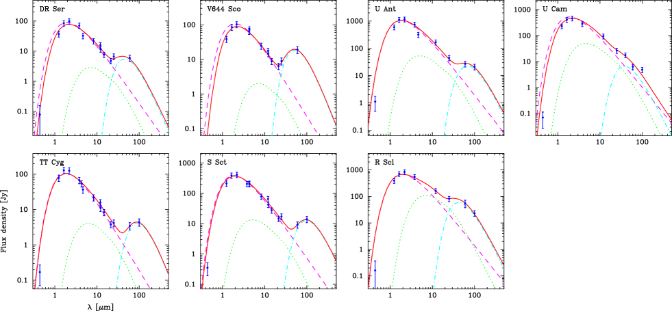
Figure 2: Observed SEDs for the seven carbon stars with detected detached molecular shells. Best-fit models to the observed SEDs are overlayed (solid line). The model SEDs are composed of a stellar part (dashed line), a present-day wind (dotted line), and a detached shell (dash-dotted line). The model SEDs have been corrected for interstellar extinction. Stellar and envelope parameters are summarized in Tables 3 and 4.

2.2 Continuum observations

The observed spectral energy distribution of each source is used to constrain the dust modelling. We have selected observations that contain the total source flux at a specific wavelength. In addition to IRAS fluxes (12–100 $\mu$m), near-infrared (NIR) JHKLM-photometric data have been obtained from the literature (see Kerschbaum 1999 and references therein). The IRAS and NIR data for a particular source were generally not obtained at the same epoch, while the NIR photometry data was. No reliable 100 $\mu$m IRAS flux estimates are available for DR~Ser and V644~Sco, due to cirrus contamination. For V644~Sco, DR~Ser, S~Sct, and TT~Cyg there exist observations from the Midcourse Space Experiment (MSX) in the range $8-21\mu$m which have been used in the analysis.

S~Sct has the largest detached shell of the sample sources with a diameter of approximately $140\arcsec$. This is comparable to the size of the IRAS beam at 60 $\mu$m ($120\arcsec$) and resolution effects start to become important. Groenewegen & de Jong (1994), in their modelling of S~Sct, estimated that about 30% of the flux was resolved out. Given the larger beam ($220\arcsec$) the effect at 100 $\mu$m is much lower as it is for all other sources in the sample. For this reason resolution effects has not been taken into account in the analysis.

We have obtained archival data taken by the Short Wavelength Spectrometer (SWS) onboard the Infrared Space Observatory (ISO) for U~Cam and estimated the flux at 40 $\mu$m. U~Cam is the source with the smallest detached shell of $15\arcsec$ in diameter, smaller than the ISO aperture ($17\arcsec\times 40\arcsec$) at 40 $\mu$m.

The observed SEDs are presented in Fig. 2.

3 Radiative transfer

This section describes the basic assumptions made in the analysis of the observed molecular line and continuum emission, and the methods used in the treatment of the radiative transfer.

3.1 General considerations

The CSEs are assumed to consist of two spherically symmetric components: an attached CSE (aCSE), i.e., a normal continuous AGB wind, and a detached, geometrically thin, CSE (dCSE) of constant density and temperature. Both components are assumed to be expanding at constant, but different, velocities. From the observed line spectra and SEDs it is clear that in many cases it is not easy to separate the contribution from the present-day wind and the detached shell. In these cases the parameters describing the shell need to be varied together with the mass-loss rate describing the present-day wind.

In what follows the procedures applied to determine the properties of the shells, as well as those of the present-day winds, from both continuum and millimetre line observations, are descibed.

The best fit model is found by minimizing

$$\chi^{2}=\sum^{N}_{i=1}\left[\frac{(F_{\mathrm{mod},\lambda}-F_{\mathrm{obs},\lambda})}{\sigma_{\lambda}}\right]^{2},$$ (1)

where $F_{\lambda}$ is the flux, and $\sigma_{\lambda}$ the uncertainty in the measured flux, at wavelength $\lambda$, and the summation is done over $N$ independent observations.

3.2 Molecular line modelling

A detailed non-LTE radiative transfer code, based on the Monte Carlo method (Bernes 1979), is used to perform the excitation analysis and to model the observed circumstellar line emission. The code is described in detail in Schöier & Olofsson (2001) and has been benchmarked, to high accuracy, against a wide variety of molecular line radiative transfer codes in van Zadelhoff et al. (2002) and van der Tak et al. (in prep.).

The excitation analysis includes radiative excitation through vibrationally excited states, and a full treatment of line overlaps between various hyperfine components in the case of HCN, see e.g. Lindqvist et al. (2000). Relevant molecular data are summarized in Schöier et al. (2005) and are made publicly available at http://www.strw.leidenuniv.nl/$\sim$moldata.

Table 3: Stellar properties.

$$\begin{array}[]{p{0.25\linewidth}ccccccccc}\hline\cr\vskip 3.0pt plus 1.0pt minus 1.0pt\cr\lx@intercol\mathrm{Source}\hfil\lx@intercol&\lx@intercol\hfil\mathrm{Var.\ type}\hfil\lx@intercol&&\lx@intercol\hfil P\hfil\lx@intercol&&\lx@intercol\hfil D\hfil\lx@intercol&&\lx@intercol\hfil L_{\star}\hfil\lx@intercol&&\lx@intercol\hfil T_{\star}\hfil\lx@intercol\\ &&&\lx@intercol\hfil\mathrm{[days]}\hfil\lx@intercol&&\lx@intercol\hfil[\mathrm{pc}]\hfil\lx@intercol&&\lx@intercol\hfil[\mathrm{L}_{\sun}]\hfil\lx@intercol&&\lx@intercol\hfil[\mathrm{K}]\hfil\lx@intercol\\ \vskip 3.0pt plus 1.0pt minus 1.0pt\cr\hline\cr\vskip 3.0pt plus 1.0pt minus 1.0pt\cr R Scl&\mathrm{SRb}&&370&&290^{2}&&4300&&2625\\ U Cam&\mathrm{SRb}&&400&&430^{2}&&7000&&2695\\ U Ant&\mathrm{Lb}&&\mbox{---}&&260^{1}&&5800&&2810\\ V644 Sco&\mathrm{Lb}&&\mbox{---}&&700^{3}&&4000&&2615\\ DR Ser&\mathrm{Lb}&&\mbox{---}&&760^{3}&&4000&&2650\\ S Sct&\mathrm{SRb}&&148&&400^{1}&&4900&&2755\\ TT Cyg&\mathrm{SRb}&&118&&610^{1}&&3200&&2825\\ \vskip 3.0pt plus 1.0pt minus 1.0pt\cr\hline\cr\end{array}$$

¹ Hipparcos distance (Knapp et al. 2003)
² From period-luminosity relation (Knapp et al. 2003)
³ From adopting $L_{\star}$ = 4000 L_⊙

3.3 Continuum modelling

An independent estimate of the properties of the detached shell and the present-day wind can be made from the excess emission observed at wavelengths longer than $\approx$ 5 $\mu$m and 20 $\mu$m, respectively. The dust emissions from both the shell and the present-day wind are expected to be optically thin at all relevant wavelengths ($\gtrsim$ 1 $\mu$m). The assumption of optically thin emission greatly simplifies the radiative transfer of the continuum emission. The simple model presented in detail below has been verified against a full radiative transfer code (Schöier, in prep.) for the densest winds encountered in this project, and they are found to agree within the numerical accuracy of the code itself ($\lesssim 5\%$).

In the optically thin limit the contribution to the SED can be separated into a stellar component $F^{\mathrm{star}}_{\nu}$, a component from the present-day wind $F_{\nu}^{{\mathrm{wind}}}$, and that from the detached shell $F_{\nu}^{{\mathrm{shell}}}$, which are solved for individually. The total SED is then obtained from $F_{\nu}=F^{\mathrm{star}}_{\nu}+F_{\nu}^{{\mathrm{wind}}}+F_{\nu}^{{\mathrm{shell}}}$ (note that the violation of energy conservation introduced in this way is negligible, $\lesssim$ 5%). Note that we ignore any beam filling effects (see Sect. 2.2).

The flux $F_{\nu}^{\mathrm{wind}}$ received by an observer located at a distance $D$ from an expanding, spherically symmetric wind produced by a constant rate of mass-loss is

$$F_{\nu}^{{\mathrm{wind}}}=\frac{4\pi^{2}a^{2}_{\mathrm{gr}}Q_{\nu}}{D^{2}}\int^{R_{\mathrm{e}}}_{R_{\mathrm{i}}}n_{\mathrm{dust}}(r)B_{\nu}(T_{\mathrm{dust}}(r))r^{2}\mathrm{d}r,$$ (2)

where $Q_{\nu}$ is the absorption efficiency of a spherical dust grain with radius $a_{\mathrm{gr}}$, $n_{\mathrm{dust}}$ the number density of dust grains, $B_{\nu}$ the blackbody brightness at the dust temperature $T_{\mathrm{dust}}$, and the integration is made from the inner ($R_{\mathrm{i}}$) to the outer ($R_{\mathrm{e}}$) radius of the CSE.

For an extended, geometrically thin, isothermal shell at constant density, adequate for describing the detached shells treated here, Eq. (2) reduces to

$$F_{\nu}^{{\mathrm{shell}}}=\frac{9Q_{\nu}}{4a_{\mathrm{g}r}\rho_{\mathrm{gr}}D^{2}}B_{\nu}(T_{\mathrm{dust}})M_{\mathrm{dust}},$$ (3)

where the dust mass of the shell, $M_{\mathrm{dust}}$, and the specific density of a grain, $\rho_{\rm gr}$, have been introduced.

The local dust temperature, $T_{\mathrm{dust}}(r)$, is determined by balancing the heating ($H$) provided by absorption of infalling radiation and cooling ($C$) by subsequent re-emission. The heating term can be expressed as

$$H=\pi a^{2}_{\mathrm{gr}}n_{\mathrm{dust}}(r)\int F^{\mathrm{star}}_{\nu}(r)Q_{\nu}\mathrm{d}\nu,$$ (4)

where the dust grains are assumed to be of the same size and spherical. The dust grains are assumed to locally radiate thermal emission according to Kirchoff’s law and the resulting cooling term is

$$C=4\pi^{2}a^{2}_{\mathrm{gr}}n_{\mathrm{dust}}(r)\int B_{\nu}(T_{\mathrm{dust}}(r))Q_{\nu}\mathrm{d}\nu.$$ (5)

Modelling the SED provides information only on the density structure of the dust grains, $\propto\dot{M}_{\mathrm{dust}}/v_{\mathrm{dust}}$, where $\dot{M}_{\mathrm{d}}$ is the dust-mass-loss rate and $v_{\mathrm{dust}}$ the dust velocity. In order to calculate $\dot{M}_{\mathrm{dust}}$, and eventually the gas mass-loss rate $\dot{M}_{\mathrm{gas}}$, one has to rely upon some model describing the dynamics of the wind. There are now growing evidence that the winds of AGB stars are driven by radiation pressure from stellar photons exerted on dust grains. Through momentum-coupling between the dust and gas, molecules are dragged along by the grains. The stationary solution to such a problem has been extensively studied (e.g., Habing et al. 1994). The terminal (at large radii) gas velocity, $v_{\mathrm{gas}}$, is given by

$$v_{\mathrm{gas}}=\sqrt{2GM_{\star}(\Gamma-1)/r_{0}},$$ (6)

where $G$ is the gravitational constant, $M_{\star}$ the stellar mass, $L_{\star}$ the luminosity, and $\Gamma$ the ratio of the drag force and the gravitational force on the gas, given by

$$\Gamma=\frac{3(Q_{\mathrm{F}}/a_{\mathrm{gr}})L_{\star}\Psi}{16\pi GcM\rho_{\mathrm{gr}}}\frac{v_{\mathrm{gas}}}{v_{\mathrm{dust}}},$$ (7)

where $Q_{\mathrm{F}}$ is the flux-averaged momentum-transfer efficiency, $c$ the speed of light, and $\Psi$ the dust-to-gas mass-loss-rate ratio. The drift velocity $v_{\mathrm{dr}}=v_{\mathrm{dust}}-v_{\mathrm{gas}}$ can be obtained from

$$v_{\mathrm{dr}}=\sqrt{\frac{v_{\mathrm{gas}}Q_{\mathrm{F}}L_{\star}}{c\dot{M}_{\mathrm{gas}}}}.$$ (8)

In the modelling, amorphous carbon dust grains with the optical constants presented in Suh (2000) were adopted. The properties of these grains were shown to reproduce, reasonably well, the SEDs from a sample of carbon stars. For simplicity, the dust grains are assumed to be spherical and of the same size with $a_{\mathrm{gr}}$ = 0.1 $\mu$m and $\rho_{\rm gr}$ = 2 g cm^-3. The absorption and scattering efficiencies were then calculated using standard Mie theory (Bohren & Huffman 1983). For the dynamical solution we further assume a stellar mass of $M$ = 1 M_⊙ and adopt an inner radius of the envelope $r_{0}$ = 8$\times$10¹³ cm (corresponding to a dust condensation temperature of $\approx$ 1200 K).

4 Dust modelling

The state of the dust grains will have a great impact on the gas modelling, affecting both its dynamics and molecular excitation. However, the reverse is not true so the dust modelling can safely be done without bothering about the state of the gas, except for the terminal gas velocity which enters in the solution of the dynamics and allows the total mass-loss rate to be estimated. Fortunately, the terminal gas velocity is an observable.

4.1 Stellar parameters

The first step in the modelling is to determine the luminosity (alternatively, the distance) from fitting the SED shortward of $\approx$ 10 $\mu$m where the stellar emission fully dominates in these optically thin envelopes. The stellar emission, $F_{\nu}^{\mathrm{star}}$, is assumed to be that of a blackbody. The stellar effective temperatures, $T_{\star}$, for our sample sources were adopted from Bergeat et al. (2001). Accurate Hipparcos parallaxes exist only for U~Ant, S~Sct, and TT~Cyg (Knapp et al. 2003), and other means of determining the distance to the remaining objects need to be adopted. For R~Scl and U~Cam we used the period-luminosity relation by Knapp et al. (2003) to obtain the distances, adopting the periods listed by Kholopov et al. (1985) and Knapp et al. (2003). The distances to the irregular variables V644~Sco and DR~Ser were obtained after adopting a luminosity of 4000 L_⊙. All the stellar parameters are listed in Table 3. In the fitting procedure, interstellar extinction was accounted for by adopting the extinction law of Cardelli et al. (1989) and using the vales for extinction in the visual, $A_{\mathrm{V}}$, listed in Bergeat et al. (2001).

4.2 Detached shell and present-day wind

The observational constraints, in the form of SEDs covering the wavelength range $\approx$ 10 $-$ 100 $\mu$m are analyzed using the $\chi^{2}$-statistic defined in Eq. (1). A calibration uncertainty of 20% was added to the total error budget and will, in most cases, dominate the error which in turn means that fluxes at various wavelengths typically have the same weight in the $\chi^{2}$-analysis. It should be noted that the present-day mass loss is more difficult to estimate than the properties of the detached shell given its lower contrast with respect to the stellar contribution.

For the present-day wind there is only one adjustable parameter in the modelling, the gas-mass-loss rate. The emission from the shell is fully described by adjusting the temperature of the dust grains ($T_{\mathrm{dust}}$) and the total dust mass in the shell ($M_{\mathrm{dust}}$). The best fit models all have reduced $\chi^{2}$ values of $\approx 1$, indicating good fits. The parameters obtained are listed in Table 4. The dust-to-gas ratio ($\Psi$) in the present-day wind obtained from the dynamical model is also listed. The sensitivity of the results to the adjustable parameters are illustrated in Fig. 3 for the young shell around DR~Ser and the older shell around TT~Cyg. The final fits to the observed SEDs are presented in Fig. 2, where also the contribution of each of the three components (stellar, present-day wind, and detached shell) are indicated.

The dust temperature in the shell can be translated into a radial distance of the shell from balancing the heating [Eq. (4)], provided by the central star, and the cooling [Eq. (5)], provided by the re-emission of the observed photons at longer wavelengths, as in the case of the present-day wind. The distances obtained are given in Table 4. As shown in Fig. 4, although the errors involved are quite large, there is a clear correlation between the radial distance of the shell and its mass, $M_{\mathrm{dust}}\propto R_{\mathrm{s}}^{1.36\pm 0.53}$. Pearson’s correlation coefficient $r$ is 0.97 indicating an almost complete positive correlation. The fact that the mass increases with distance suggests that matter is being swept up as the shell expands away from the star. Such a scenario will be further elaborated in Sect. 6.1.

U~Cam is the source which has the lowest contrast between the stellar and shell contributions to the SED. It is the youngest shell in the sample located close to the central star, Sect. 5., complicating also its separation from the present day wind. This makes it hard from the dust modelling to constrain the properties of the circumstellar dust for this particular source.

Groenewegen & de Jong (1994) modelled the SED of S~Sct and found a shell dust mass of $\approx$ 2$\times$10^-4 M_⊙. Given the uncertainties in the adopted dust properties, this is consistent with the mass derived in the present analysis. Placing the dust shell at the same location as that of CO we derive a dust mass of $\approx$ 8$\times$10^-5 M_⊙ for our somewhat smaller distance.

Izumiura et al. (1997) in their analysis of HIRAS images found evidence for two separate dust shells around U~Ant where the inner of the two shells is coinciding with that of CO. They derive a total mass for this shell of $\approx$ 5$\times$10^-3 M_⊙ consistent within the uncertainties with our estimate of $\approx$ 2$\times$10^-3 M_⊙ from the CO modelling. The outer shell, which has no known molecular counterpart, is similarly thought to have been produced in another thermal pulse some $\sim$ 10⁴ yr before. The dust mass contained in this shell is estimated to be $\approx$ 4$\times$10^-5 M_⊙ and its contribution to the SED is $\approx$ 15% at 60 $\mu$m.

Table 4: Results from dust modelling (with 1$\sigma$ errors)

.

$$\begin{array}[]{p{0.15\linewidth}cccccccccccc}\hline\cr\vskip 3.0pt plus 1.0pt minus 1.0pt\cr&\lx@intercol\hfil\mathrm{dCSE}\hfil\lx@intercol&&&&\lx@intercol\hfil\mathrm{aCSE}\hfil\lx@intercol\\ \cline{2-6}\cr\cline{10-12}\cr\lx@intercol\mathrm{Source}\hfil\lx@intercol&\lx@intercol\hfil M_{\mathrm{dust}}\hfil\lx@intercol&&\lx@intercol\hfil T_{\mathrm{dust}}\hfil\lx@intercol&&\lx@intercol\hfil R_{\mathrm{s}}\hfil\lx@intercol&&&&\lx@intercol\hfil\dot{M}_{\mathrm{gas}}\hfil\lx@intercol&&\lx@intercol\hfil\Psi\hfil\lx@intercol\\ &\lx@intercol\hfil[\mathrm{M}_{\sun}]\hfil\lx@intercol&&\lx@intercol\hfil[\mathrm{K}]\hfil\lx@intercol&&\lx@intercol\hfil[\mathrm{cm}]\hfil\lx@intercol&&&&\lx@intercol\hfil[\mathrm{M}_{\sun}\,{\mathrm{yr}}^{-1}]\hfil\lx@intercol&&\\ \vskip 3.0pt plus 1.0pt minus 1.0pt\cr\hline\cr\vskip 3.0pt plus 1.0pt minus 1.0pt\cr R Scl&(3.2\pm 2.0)\times 10^{-5}&&75\pm 15&&(1.2\pm 0.6)\times 10^{17}&&&&{\phantom{<}}3.8\times 10^{-7}&&1.7\times 10^{-3}\\ U Cam&1.5\times 10^{-6}-1.0\times 10^{-3}&&70\pm 45&&\mbox{---}&&&&{\phantom{<}}4.0\times 10^{-7}&&1.2\times 10^{-3}\\ U Ant&(1.3\pm 1.2)\times 10^{-4}&&55\pm 20&&(5.1\pm 4.0)\times 10^{17}&&&&{\phantom{<}}7.0\times 10^{-8}&&3.0\times 10^{-3}\\ V644 Sco&(1.4\pm 0.9)\times 10^{-4}&&61\pm 9\phantom{0}&&(1.8\pm 0.7)\times 10^{17}&&&&<5.0\times 10^{-8}&&\mbox{---}\\ DR Ser&(3.5\pm 2.5)\times 10^{-5}&&68\pm 13&&(1.5\pm 0.7)\times 10^{17}&&&&<7.0\times 10^{-8}&&\mbox{---}\\ S Sct&(8.0\pm 7.0)\times 10^{-4}&&34\pm 9\phantom{0}&&(1.3\pm 0.8)\times 10^{18}&&&&<8.0\times 10^{-8}&&\mbox{---}\\ TT Cyg&(4.3\pm 3.7)\times 10^{-4}&&39\pm 10&&(6.9\pm 4.1)\times 10^{17}&&&&<3.2\times 10^{-8}&&\mbox{---}\\ \vskip 3.0pt plus 1.0pt minus 1.0pt\cr\hline\cr\end{array}$$

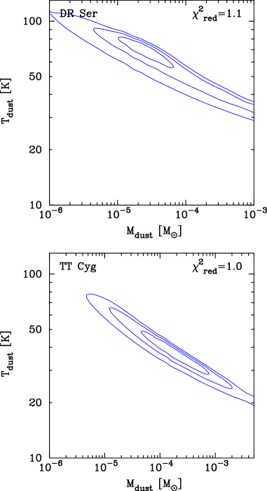
Figure 3: $\chi^{2}$-maps showing the sensitivity of the adjustable parameters $T_{\mathrm{dust}}$ and $M_{\mathrm{dust}}$ in the dust modelling of the detached shells around DR~Ser and TT~Cyg. Contours are drawn at $\chi^{2}_{\mathrm{min}}+(2.3,6.2,11.8)$ indicating the 68% (‘1$\sigma$’), 95% (‘2$\sigma$’), and 99.7% (‘3$\sigma$’) confidence levels, respectively. The quality of the best fit model can be estimated from the reduced chi-squared statistic $\chi^{2}_{\mathrm{red}}$=$\chi^{2}_{\mathrm{min}}$/($N$$-$2) shown in the upper right corner.

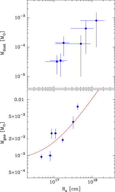
Figure 4: The shell dust ($M_{\mathrm{dust}}$; upper panel) and gas ($M_{\mathrm{gas}}$; lower panel) masses plotted as a function of the radius of the shell ($R_{\mathrm{s}}$). The solid line shows the mass-radius relation of the interacting wind model presented in Sect. 6.2.

5 Molecular line modelling

5.1 Line profiles

Many of the observed CO spectra exhibit a triple-peaked line profile, e.g., Olofsson et al. (1996). The, usually narrow, peaks at the extreme velocities arise from a spatially resolved shell, whereas the central component is produced by the present-day wind, i.e., a normal low-mass-loss-rate AGB wind. Since the present-day wind is in general expanding at a significantly lower velocity, $v_{\rm p}$, than that of the shell, $V_{\rm s}$, emission at velocities between $v=v_{\star}\pm v_{\rm p}$ and $v=v_{\star}\pm V_{\rm s}$ should contain only the contribution from the shell. Each of these velocity intervals is further divided into two separate components so that the total $\chi^{2}$-statistic also contains information on the line profile.

Information on the properties of the present-day mass-loss rate is contained in the intensity in the range $v=v_{\star}\pm v_{\rm p}$. However, there is also generally a contribution here from the detached shell and a good model for the shell is required in order to investigate the present-day wind. This makes it particularly difficult to separate the two components in all cases except U~Ant, S~Sct, and TT~Cyg, (e.g., Olofsson et al. 1996). In the case of U~Cam the present-day wind is separated in the CO line interferometer data (Lindqvist et al. 1999). In the cases of R~Scl, V644~Sco, and DR~Ser the detected HCN emissions indicate expansion velocities about a factor of two lower than in the case of the CO emission. The HCN emission is interpreted as arising predominantly in the present-day wind. This was also the conclusion reached by Wong et al. (2004) for R~Scl.

Table 5: Results from molecular line modelling (with 1$\sigma$ errors bars)

.

$$\begin{array}[]{p{0.15\linewidth}ccccccccccccc}\hline\cr\vskip 3.0pt plus 1.0pt minus 1.0pt\cr&\lx@intercol\hfil\mathrm{dCSE}\hfil\lx@intercol&&&&\lx@intercol\hfil\mathrm{aCSE}\hfil\lx@intercol\\ \cline{2-8}\cr\cline{12-14}\cr\lx@intercol\mathrm{Source}\hfil\lx@intercol&\lx@intercol\hfil M_{\mathrm{gas}}\hfil\lx@intercol&&\lx@intercol\hfil T_{\mathrm{kin}}\hfil\lx@intercol&&\lx@intercol\hfil R_{\mathrm{s}}\hfil\lx@intercol&\lx@intercol\hfil V_{\mathrm{s}}\hfil\lx@intercol&\lx@intercol\hfil\mathrm{age}\hfil\lx@intercol&&&&\lx@intercol\hfil\dot{M}_{\mathrm{gas}}\hfil\lx@intercol&\lx@intercol\hfil v_{\mathrm{p}}\hfil\lx@intercol&\lx@intercol\hfil\mathrm{Molecule}^{1}\hfil\lx@intercol\\ &\lx@intercol\hfil[\mathrm{M}_{\sun}]\hfil\lx@intercol&&\lx@intercol\hfil[\mathrm{K}]\hfil\lx@intercol&&\lx@intercol\hfil[\mathrm{cm}]\hfil\lx@intercol&\lx@intercol\hfil[\mathrm{km\,s}^{-1}]\hfil\lx@intercol&\lx@intercol\hfil[\mathrm{yr}]\hfil\lx@intercol&&&&\lx@intercol\hfil[\mathrm{M}_{\sun}\,{\mathrm{yr}}^{-1}]\hfil\lx@intercol&\lx@intercol\hfil[{\mathrm{km}}\,{\mathrm{s}}^{-1}]\hfil\lx@intercol&\\ \vskip 3.0pt plus 1.0pt minus 1.0pt\cr\hline\cr\vskip 3.0pt plus 1.0pt minus 1.0pt\cr R Scl&(2.5\pm 0.5)\times 10^{-3}&&>20\phantom{0}&&8.7\times 10^{16}&15.5&1800&&&&3.0\times 10^{-7}&10.5&\mathrm{HCN}\\ U Cam&(9.5\pm 1.0)\times 10^{-4}&&>130&&4.7\times 10^{16}&23.0&\phantom{0}650&&&&2.0\times 10^{-7}&12.0&\mathrm{CO}\\ U Ant&(1.9\pm 0.2)\times 10^{-3}&&>200&&1.7\times 10^{17}&19.0&2800&&&&2.0\times 10^{-8}&\phantom{0}4.0&\mathrm{CO}\\ V644 Sco&(2.5\pm 0.3)\times 10^{-3}&&170\pm 100&&(1.1\pm 0.2)\times 10^{17}&23.0&1500&&&&5.0\times 10^{-8}&\phantom{0}5.0&\mathrm{HCN}\\ DR Ser&(1.0\pm 0.2)\times 10^{-3}&&>100&&(8.0\pm 1.5)\times 10^{16}&20.0&1300&&&&3.0\times 10^{-8}&\phantom{0}5.0&\mathrm{HCN}\\ S Sct&(7.5\pm 1.0)\times 10^{-3}&&>60\phantom{0}&&4.2\times 10^{17}&16.5&8100&&&&2.0\times 10^{-8}&\phantom{0}4.0&\mathrm{CO}\\ TT Cyg&(4.0\pm 1.0)\times 10^{-3}&&>200&&3.2\times 10^{17}&12.5&8100&&&&3.2\times 10^{-8}&\phantom{0}4.0&\mathrm{CO}\\ \vskip 3.0pt plus 1.0pt minus 1.0pt\cr\hline\cr\end{array}$$

¹ The molecular line emission used for estimating the properties of the aCSEs. Note that in the analysis of the dCSEs CO line emission was used in all cases.

5.2 The detached shells

In the analysis there exist four adjustable parameters: the H₂ number density ($n_{\mathrm{H}_{2}}$), kinetic gas temperature ($T_{\mathrm{kin}}$), thickness ($\Delta R_{\mathrm{s}}$) and location of the shell ($R_{\mathrm{s}}$). The fractional abundance of CO (in relation to H₂), $f_{\mathrm{CO}}$, is assumed to be equal to 1.0$\times$10^-3. In three cases (TT Cyg, Olofsson et al. (2000); U Cam, Lindqvist et al. (1999); S Sct, Olofsson et al., in prep.) the sizes of the shells are well known from interferometric CO observations. In the case of U Ant the size of the shell is reasonably well known from single-dish CO mapping. R~Scl has a prominent detached shell at $\approx$ 8.7$\times$10¹⁶ cm seen in scattered light (González Delgado et al. 2001). In these five cases the position of the shell was fixed to match the observations. Although high-spatial-resolution observations exist, little is known about the actual thickness of these shells. CO interferometric observations do not resolve the radial thickness of the shells. Here we adopt a value of 1.0$\times$10¹⁶ cm. The best-fit model is found from minimizing the $\chi^{2}$-statistic as described above.

As an example, in Fig. 5 $\chi^{2}$-maps obtained from the modelling of the shell around V644~Sco are shown. The location of the shell ($R_{\mathrm{s}}$) is unknown and used as an adjustable parameter. However, it turns out that the shell radial distance from the central star is the best constrained parameter in the modelling, together with the mass contained in the shell. Fig. 5 (lower panel) shows the sensitivity of the model to changes in $R_{\mathrm{s}}$ and $n_{\mathrm{H_{2}}}$ for a fixed temperature of 100 K. In a broad temperature range we find that good fits are obtained for $R_{\mathrm{s}}$=(1.1$\pm$0.2)$\times$10¹⁷ cm. Fixing the radial distance to 1.1$\times$10¹⁷ cm, the density and temperature are constrained to $1050\pm 150$ cm^-3 and $170\pm 100$ K, respectively (Fig. 5; upper panel). The mass contained in the shell is $M_{\mathrm{gas}}$ = (2.5$\pm$0.3)$\times$10^-3 M_⊙.

The derived mass in the shell is not very sensitive to the adopted thickness of the shell since the emission in almost all observed lines is optically thin. The density in the shell, however, goes roughly as $n_{\mathrm{H_{2}}}$ $\propto$ $\Delta R_{\mathrm{s}}^{-1}$. There is also a weak temperature dependence.

The CO line emission from the lower rotational transitions is not very sensitive to changes in the kinetic gas temperature once $T_{\mathrm{kin}}$ $>$ 50 $-$ 100 K. In order to better constrain the temperature in the shell transitions involving higher $J$-levels needs to be observed as illustrated in Sect. 6.4.

The properties of all dCSEs determined from the CO line modelling are summarized in Table 5. Fig. 4 illustrates that, as in the case of the dust emission, there is a clear trend that the gas mass of the shell increases with its radial distance from the central star. Again a strong correlation is found $M_{\mathrm{gas}}\propto R_{\mathrm{s}}^{0.85\pm 0.18}$ ($r=0.93$) further supporting a scenario where matter is being swept up as discussed in Sect. 6.1. Also in indicated in Table 5 is the age of the dCSEs estimated from $R_{\mathrm{s}}/V_{\mathrm{s}}$. Since there is a clear trend that $V_{\mathrm{s}}$ decrease with $R_{\mathrm{s}}$ (Sect. 6.1) these ages are strictly upper limits to the age since the expansion was likely faster at earlier epochs.

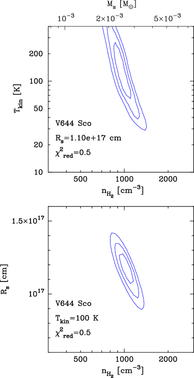
Figure 5: $\chi^{2}$-maps showing the sensitivity of the adjustable parameters $n_{\mathrm{H_{2}}}$, $T_{\mathrm{kin}}$, and $R_{\mathrm{s}}$ in the CO modelling of the detached shell around V644~Sco. Contours are drawn at $\chi^{2}_{\mathrm{min}}+(2.3,6.2,11.8)$ indicating the 68% (‘1$\sigma$’), 95% (‘2$\sigma$’), and 99.7% (‘3$\sigma$’) confidence levels, respectively. The quality of the best fit model can be estimated from the reduced chi-squared statistic $\chi^{2}_{\mathrm{red}}$=$\chi^{2}_{\mathrm{min}}$/($N$$-$2) shown in the lower left corner. Also indicated is the value of the parameters that is kept fixed in these maps.

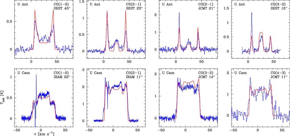
Figure 6: Best fit models (solid line) including both the present-day wind and detached shell emission overlayed on observed spectra (histograms) for U~Ant and U~Cam. The uncertainty in the intensity scale is $\pm 20$%. The narrow spikes found near the blue wing in the spectra of U Cam are of interstellar origin.

5.3 The present-day winds

Once the properties of the detached shell are determined and its contribution to the observed CO line emission is estimated, the corresponding estimates for the present-day wind can be can be made. In the modelling of the present-day wind the temperature structure is solved for self-consistently as described in Schöier & Olofsson (2001) using the results from the dust modelling performed in Sect. 4 to describe the properties of the dust entering in the heating of the gas envelope. It should be emphasised that the actual CO line intensities are not very sensitive to the temperature structure since the excitation is dominated by the radiation field from the central star in these low-mass-loss-rate objects (Schöier & Olofsson 2001).

Adopting a CO abundance of 1.0$\times$10^-3 relative to H₂ leaves just the mass-loss rate, $\dot{M}_{\mathrm{gas}}$, as an adjustable parameter in the modelling. The expansion velocity of the present-day wind is fixed from matching the observed lines with the model (assuming a micro-turbulent line broadening of $1.0$ km s^-1, in addition to the thermal motion). The CO envelope size is calculated from the photodissociation model of Mamon et al. (1988). The applicability of these results to the present-day wind in these objects is a bit questionable since the shell itself may provide shielding against photodissociation. In the modelling, the CO $J=1\rightarrow 0$ intensity is most sensitive to the size of the envelope (Schöier & Olofsson 2001).

For some of the younger detached shell sources like R~Scl, V644~Sco, and DR Ser it is difficult, given the current set of CO observations available, to estimate reliable mass-loss rates. In these objects the observed HCN line emission has been used instead. HCN is only probing the present-day wind since it is readily photodissociated at the distances where the detached shells are found. Note, however, that there is some indication that HCN $J=1\rightarrow 0$ emission from the shell is detected in V644~Sco (Fig. 1). As in the case of the CO modelling an assumption of the HCN abundance distribution needs to be made in order to estimate the mass-loss rate. HCN is a species with a photospheric origin. Olofsson et al. (1993a) estimated HCN abundances in the photospheres of four of the sample stars and obtained values of $\sim 0.8-5.4\times 10^{-5}$ relative to H₂. Here we adopt a generic value of $2\times 10^{-5}$ for the analysis. The size of the HCN envelope was then calculated from a photodissociation model based on the results from Lindqvist et al. (2000). It should be pointed out that for each HCN model a CO model using the same mass-loss rate needs to be calculated first in order to obtain the correct temperature profile to use. This also makes it possible to check if the CO model is consistent with the observed CO lines. In all three cases it is.

U~Cam is the only source where the abundance of HCN in the aCSE can be determined based on the results from the CO modelling. Using the mass-loss rate and expansion velocities from Table 5, an HCN abundance of approximately $4\times 10^{-5}$ (relative to that of H₂) is obtained using the results from Lindqvist et al. (2000) to calculate the HCN envelope size. A more detailed investigation of the HCN and CN envelopes around U~Cam based on new high-spatial-resolution interferometric observations is underway (Lindqvist et al., in prep.). U Cam, together with V644 Sco, are the only sources where HCN emission from the detached shell is detected.

The expansion velocities and derived mass-loss rates for the present-day wind (aCSE) are presented in Table 5. The uncertainties in the mass-loss-rate estimates, within the adopted circumstellar model, are about $\pm 50\%$ for estimates based on CO observations and as high as a factor $\sim 5$ when HCN emission is used, mainly due to the larger uncertainty in the adopted photospheric HCN abundance. Examples of line profiles taken from the best-fit models, including both contribution from the present day wind and detached shell, are given in Fig. 6 for U~Cam and U~Ant.

In Fig. 7 the present-day-wind mass-loss rates and gas expansion velocities are plotted against the size of the detached shell. Even though the uncertainties in the mass-loss rates are substantial (particularly those based on HCN emission) we conclude that there is a trend of decreasing present-day mass-loss rate with increasing size of the shell. This is further corroborated by the similar decrease in the gas expansion velocity with increasing size of the shell. The velocity is an observational property that can be determined with high accuracy, and it is known to correlate reasonably well with the mass-loss rate for ‘normal’ CSEs (e.g., Olofsson 2003). The implications of this result is further discussed in Sect. 6.

5.4 The detached shell around R~Scl

R~Scl deserves a separate discussion. From the dust modelling it appears to be a normal detached shell source (see Table 4). However, the CO line modelling of the main isotope places the shell at about half the distance of what is actually determined from scattered-light observations (González Delgado et al. 2001). The mass of the shell is also unusually high $\approx$ 1.0$\times$10^-2 M_⊙ for such a young shell. Modelling of the rarer ¹³CO isotopomer, however, gives results consistent with the larger radial position of the shell, and a much lower shell mass of approximately 2.5$\times$10^-3 M_⊙ is obtained [adopting the photospheric ¹²C/¹³C ratio of 19 determined by Lambert et al. (1986)]. The properties of the detached shell around R~Scl reported in Table 5 are based on the ¹³CO modelling.

The reason for the discrepancy obtained from the ¹²CO modelling is not known. Possibly, the mass-loss-rate history of this object is more complicated. Therefore, detailed interferometric CO observations are important for resolving this issue.

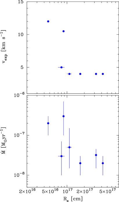
Figure 7: The present-day-wind gas expansion velocity (upper panel) and mass-loss rate (lower panel) plotted as a function of the radius of the shell ($R_{\mathrm{s}}$).

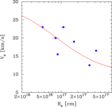
Figure 8: The shell expansion velocity ($V_{\mathrm{s}}$) plotted against the shell radius ($R_{\mathrm{s}}$; as determined from CO line data). The solid line shows the expected velocity-radius relation of the interacting wind model presented in Sect. 6.2

.

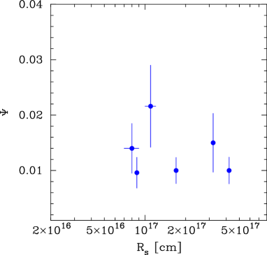
Figure 9: The dust-to-gas ratio ($\Psi$) plotted against the radius of the shell ($R_{\mathrm{s}}$; assuming that the dust and gas shells coincide spatially).

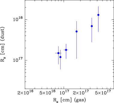
Figure 10: Relation between the radius of the shell as determined from dust and gas modelling, respectively.

6 Discussion

6.1 Evidence for interacting winds

As shown in Fig. 4 there is compelling evidence from both the dust and gas modelling that a detached shell gains mass as it expands away from the central star. This would indicate that material is being swept up in the process. Further support for such a scenario comes from the observed width of the CO line emission emanating from the shell. Fig. 8 shows a correlation ($r$ = $-0.64$) between the expansion velocity of the shell, $V_{\mathrm{s}}$, and its location, $R_{\mathrm{s}}$ in that the farther away the shell is located the lower its velocity. This could be naturally explained if the shell is indeed interacting with some other medium. In addition, the high inferred kinetic temperatures (actually lower limits) are also a signpost of interaction.

The strongest argument for the $M_{\rm s}$–$R_{\rm s}$ relation is that it is obtained in two completely independent ways. Nevertheless, the possibilities of systematic errors in the analysis and observational biases should be investigated. One way of looking for possible systematic errors in the analysis, which also includes both the dust and the gas estimates, is to calculate the dust-to-gas mass-loss-rate ratio ($\Psi$) in the shells. To do this we have placed both the gas and dust shells at the same radial distance. The resulting values for $\Psi$ as a function of the radial distance of the shell are shown in Fig. 9. There is no apparent correlation ($r$ $=$ 0.49) between the two quantities, and the results are consistent with the same value of $\Psi$ in all the shells, $\approx$ 0.012. This result provides no indication of a systematic error. On the other hand, the dust-to-gas mass-loss-rate ratios derived for the present day winds (Table 4) are much lower (by a factor 3-10) than those found for the shells, but fully consistent with those normally quoted for low to intermediate mass-loss-rate carbon stars (Groenewegen et al. 1998). As shown by Groenewegen et al. (1998) there is a trend that the dust-to-gas ratio increases with mass-loss rate and that for $\dot{M}$ $\gtrsim$ 5$\times$10^-6 M_☉ yr^-1 (representative of the high-mass-loss-rate epoch producing the detached shell) $\Psi$ $\sim$ 0.01.

The fact that the locations of the dCSEs as determined from the dust modelling correlate very well with those estimated from CO observations, as shown in Fig. 10, suggests that the dust and gas shells are located relatively close spatially. González Delgado et al. (2003) in their study of scattered stellar light in the CSE around U~Ant found that the dust shell is located about $7\arcsec$ further out than that of CO (corresponding to a drift velocity of $\approx$ 3 km s^-1).

The most important parameter in the dust analysis is the dust temperature. The derived dust mass scales as $T_{\rm dust}^{-1}$ in the Rayleigh-Jeans limit and as $\exp(h\nu/kT_{\rm dust})$ in the Wien’s regime, and the inferred shell radius as $T_{\rm dust}^{-2.5}$ (if the grain emissivity scales as $\nu$). This means that even in the case of identical shells a spread in estimated dust temperatures will result in a mass–radius relation (with a scatter depending on the properties of the central stars). Thus, in the dust analysis the accuracy of the dust temperature estimate is crucial. As shown in Table 4 these are rather well constrained (even though longer-wavelength data, free of cirrus contamination, are highly desirable), and we conclude that the dust temperature estimates are not the reason for the mass-radius relation.

There is possibly an observational bias in the sense that low-mass shells of large radii would be difficult to detect in both dust and CO line emission. We cannot exclude that such shells exist. On the other hand, we see no reason (other than the scarcity of stars with detached shells) why high-mass shells of small size should be missed, and are therefore reasonably certain about the upper envelope of the shell mass for a given shell size.

6.2 A simple interacting-wind scenario

Thus, we conclude that the observed mass-radius relations are most likely correct, and use a simple interacting-wind model to estimate whether our data can be explained in such a scenario using reasonable assumptions on AGB winds. Kwok et al. (1978) presented the results of a fully momentum-coupled wind interaction. In the model a fast moving wind is running into a slower moving wind. Both winds are assumed to be spherically symmetric, have constant mass-loss rates, and expand at constant velocities. The qualitative validity of this simple picture has been verified by detailed modelling performed by Steffen & Schönberner (2000).

In our case it should be noted that the high velocities observed for the younger detached shell sources strongly suggests that the mass-loss rate forming the fast moving wind was also very high, say about 10^-5 M_⊙ yr^-1, since the mass-loss rate and gas expansion velocity correlates positively for normal CSEs (e.g., Olofsson 2003). Based on Fig. 4 it is reasonable to assume that the initial mass of the shell is of the order 10^-3 M_⊙, i.e., with a mass-loss rate of 10^-5 M_⊙ yr^-1 the ejection period is about 10² years. Thus, a brief period of very high mass-loss rate is inferred producing a fast moving shell.

We have modified the model of Kwok et al. (1978) to treat a scenario in which a fast moving shell is running into a slower moving wind. Conservation of the total momentum contained in the shell (both ejected and swept-up material) gives an expression for the shell velocity $V_{\mathrm{s}}$

$$V_{\mathrm{s}}=\frac{M_{\mathrm{ej}}V_{\mathrm{ej}}+M_{\mathrm{sw}}V_{\mathrm{sl}}}{M_{\mathrm{ej}}+M_{\mathrm{sw}}}$$ (9)

where $M_{\mathrm{ej}}$ is the mass contained in the initial fast moving shell at constant velocity $V_{\mathrm{ej}}$, and $V_{\mathrm{sl}}$ the constant velocity of the slower moving wind. The mass of the initial slow wind swept-up by the shell, $M_{\mathrm{sw}}$, is given by

$$M_{\mathrm{sw}}=\frac{\dot{M}_{\mathrm{sl}}}{V_{\mathrm{sl}}}R_{\mathrm{s}},$$ (10)

i.e., the shell mass ($M_{\mathrm{s}}=M_{\mathrm{ej}}+M_{\mathrm{sw}}$) will increase linearly with radius.

Assuming $V_{\mathrm{ej}}$=30 km s^-1 and $M_{\mathrm{ej}}$=8$\times$10^-4 M_⊙, further adopting the median values for the mass-loss rate and the gas expansion velocity of a sample of irregular and semiregular carbon stars, $\dot{M}_{\mathrm{sl}}$=3$\times$10^-7 M_⊙ yr^-1 and $V_{\mathrm{sl}}$=10 km s^-1 (Schöier & Olofsson 2001) as typical values for the slow wind, we find that the velocity of the shell decrease as illustrated in Fig. 8. The mass-radius relation predicted by the model is shown in Fig. 4. In all, this simple interacting wind model explains the observed properties of detached shells, bearing in mind that individual objects very likely have different characteristics.

Under the assumption that the slow stellar wind is that of a typical AGB star there is still the need of a very brief period of high mass loss also in the interacting wind scenario. These eruptive events are most likely linked to a He-shell flash (thermal pulse) as originally suggested by Olofsson et al. (1990) and Vassiliadis & Wood (1993).

It is possible that the swept-up material is depleted in CO due to it being photodissociated to some degree. This would be most pronounced for the older shells. At the densities and temperatures prevailing in the shells there are no means of effectively producing CO (Mamon et al. 1988). In this sense the estimated gas shell masses should be regarded as lower limits, in particular for the larger shells.

The cooling time scales are $\sim$ $10^{2}$ $-$ $10^{3}$ yr for gas cooling and as high as $\sim$ $10^{5}$ $-$ $10^{6}$ yr for the dust (Burke & Hollenbach 1983). Even the gas cooling time scale is rather long compared with the shell formation and dynamical time scales. However, the time scales will be significantly reduced in a clumpy medium. A clumpy medium, with gas and dust well mixed, would also explain why the dust shells show effects of swept-up material despite the fact that the dust mean-free path is rather long for the densities derived assuming homogeneous shells.

Finally, we have found evidence that the present-day mass-loss rate is decreasing with the size of the shell. The most reasonable interpretation of this is that the mass-loss rate declines to very low levels after the brief period of very high mass loss on a time scale of a few thousand years. Thus, there should be material inside the shells. There is no indication of this in the interferometer CO line maps, suggesting that here the CO molecules have been photodissociated. In the shells the densities are higher and the CO molecules survive longer. This is supported by the detections of ¹³CO in some cases. However, it should be noted that interferometers are notoriously insensitive to weak extended emission and that Lindqvist et al. (1999) and Olofsson et al. (2000) only recover about 50% of the total flux in their interferometric maps.

6.3 Photodissociation

The ¹²CO/¹³CO-ratio in the shells of V644~Sco and S~Sct are 25 and 20, respectively. For S~Sct there exist photospheric estimates of the ¹²C/¹³C-ratio. Lambert et al. (1986) have estimated this ratio to be 45, significantly larger than the value of 14 subsequently obtained by Ohnaka & Tsuji (1996) in a different analysis. The rather low values for the circumstellar ratio, and in the case of S~Sct a rough agreement with the estimated photospheric ratio, suggest that photodissociation of CO molecules is low in the shells. If photodissociation would be effective this ratio should be much higher due to the lower ability of self-shielding for the rarer ¹³CO isotopomer. The fact that the CO molecules appear to survive even out to distances of $\approx$ 5$\times$10¹⁷ cm would suggest that the medium is clumpy to a large degree, as indeed suggested by observations (Olofsson et al. 1996; Lindqvist et al. 1999; Olofsson et al. 2000).

6.4 Predictions for future sub-millimetre observations

To date only three sources have been studied in detail using interferometry. It is of importance also to map the remaining three sources, in particular R~Scl. However, high-$J$ CO observations are also useful, in particular to constrain the kinetic gas temperature in the shell. To illustrate this, predictions for high-frequency CO observations have been calculated based on the best-fit model for V644~Sco using a 15 m telescope. The results are presented in Table 6 for three different temperatures in the shell. Note that the density has been decreased slightly when the temperature was raised in order to maintain a good fit to the observed CO lines ($J=1\rightarrow 0,2\rightarrow 1,3\rightarrow 2$).

These results show the potential of single-dish telescopes such as CSO, JCMT and the upcoming APEX to further constrain the properties of detached shells.

Table 6: Predicted CO line intensities (in K km s^-1) for the detached shell around V644~Sco.

$$\begin{array}[]{p{0.3\linewidth}ccccc}\hline\cr\vskip 3.0pt plus 1.0pt minus 1.0pt\cr\lx@intercol{\mathrm{Transition}}\hfil\lx@intercol&\lx@intercol\hfil T_{\mathrm{kin}}[\mathrm{K}]\hfil\lx@intercol\\ \cline{2-6}\cr&\lx@intercol\hfil 100\hfil\lx@intercol&&\lx@intercol\hfil 200\hfil\lx@intercol&&\lx@intercol\hfil 400\hfil\lx@intercol\\ \vskip 3.0pt plus 1.0pt minus 1.0pt\cr\hline\cr\vskip 3.0pt plus 1.0pt minus 1.0pt\cr$J=1\rightarrow 0$&\phantom{0}6.5\phantom{0}&&\phantom{0}5.8\phantom{0}&&\phantom{0}5.1\phantom{0}\\ $J=2\rightarrow 1$&22.6\phantom{0}&&22.8\phantom{0}&&22.6\phantom{0}\\ $J=3\rightarrow 2$&20.7\phantom{0}&&22.9\phantom{0}&&25.5\phantom{0}\\ $J=4\rightarrow 3$&\phantom{0}7.8\phantom{0}&&12.5\phantom{0}&&13.2\phantom{0}\\ $J=6\rightarrow 5$&\phantom{0}0.58&&\phantom{0}1.2\phantom{0}&&\phantom{0}2.3\phantom{0}\\ $J=7\rightarrow 6$&\phantom{0}0.15&&\phantom{0}0.41&&\phantom{0}1.0\phantom{0}\\ $J=8\rightarrow 7$&\phantom{0}0.04&&\phantom{0}0.15&&\phantom{0}0.44\\ \vskip 3.0pt plus 1.0pt minus 1.0pt\cr\hline\cr\end{array}$$

7 Conclusions

We report the detection of a detached molecular shell around the carbon star DR~Ser. The properties of the shell are similar to the young shells found around the carbon stars U~Cam and V644~Sco. With DR~Ser the total number of carbon stars with molecular detached shells are seven. In fact, there is not much hope of increasing this number further since most of the reasonably nearby AGB stars with mass loss have already been searched for circumstellar CO radio line emission, and for the more distant objects the double-peaked line profiles become less pronounced and detached shell sources accordingly more difficult to identify. We therefore considered the time ripe for a systematic analysis of the existing objects.

Based on radiative transfer modelling of both observed molecular line emission and continuum emission the properties of the dust and gas in these shells, as well as the present-day stellar mass loss have been investigated. It turns out that there is a clear trend that both the dust and gas shell masses increase with radial distance from the central stars. At the same time the velocity by which the shells recede from the stars decreases with radial distance. The most plausible explanation for this behaviour is that the shell is sweeping up material from a surrounding medium.

We find that an interacting wind scenario where a brief period ($\sim$ 10² yr) of high mass-loss rate ($\sim$ 10^-5 M_⊙ yr^-1) results in a high-velocity shell ($\lesssim$ 30 km s^-1) that expands into a previous slow, low-mass-loss-rate AGB wind gives an adequate description of the observations. There is also evidence that the mass-loss rate, following the short period of very intense mass loss, decreases on a time scale of a few thousand years to reach a low level (a few 10^-8 M_⊙ yr^-1). The most plausible scenario for such a mass-loss-rate modulation is a He-shell flash (thermal pulse).

The gas kinetic temperature is the least well constrained parameter in the modelling. We suggest that observing high-$J$ transitions from CO using current and future single-dish telescopes should help to constrain this parameter.

Among the seven stars with known detached molecular shells, R~Scl clearly stands out. The modelling of its ¹²CO line emission suggests a shell located about a factor of two closer to the star compared with observations of scattered stellar light. Also the derived mass is significantly higher than obtained from dust and ¹³CO line modelling. This could possibly indicate that R Scl has had a significantly different mass-loss-rate history than the other detached shell sources, and this warrants further study, in particular through interferometric CO observations.