The extended Lyman-$\alpha$ emission surrounding the $z=3.04$ radio-quiet QSO1205-30: Primordial infalling gas illuminated by the quasar?

We present spectroscopic observations obtained with the FORS1 instrument on the ESO VLT under good seeing conditions of the radio-quiet $z_{\rm em}=3.04$ quasar Q1205-30 and its associated extended Ly$\alpha$ emission. The extended Ly$\alpha$ emission was originally found in a deep narrow band image targeting a $z_{\rm abs}\approx z_{\rm em}$ Lyman-limit system in the spectrum of the QSO. Using spectral point-spread function fitting to subtract the QSO spectrum, we clearly detect the extended Ly$\alpha$ emission as well as two foreground galaxies at small impact parameters ($2.12\pm 0.04$ and $2.77\pm 0.07$ arcsec). The redshifts of the two foreground galaxies are found to be $z=0.4732$ and $z=0.865$. We determine the redshift and velocity profile for the extended Ly$\alpha$ emission, and analyzing the velocity offsets between eight QSO emission lines we refine the quasar redshift determination. We use the new redshifts to infer the geometry of the complex. We find that the extended Ly$\alpha$ emission is clearly associated with the quasar. A Ly$\alpha$ luminosity of $5.6\times 10^{43}\text{\leavevmode\nobreak\ erg\leavevmode\nobreak\ s}^{-1}$ places this extended emission at the high luminosity end of the few previous detections around radio-quiet quasars. The extended Ly$\alpha$ emission is best explained by hydrogen falling into the dark matter halo inhabited by the quasar.

1 Introduction

Quasar host galaxies are visible tracers of the close environment of this powerful type of active galactic nuclei (AGN). The feeding of the central engine from the host galaxy, and the feedback of the quasar to the host are important unknown factors in current numerical models, which need to be understood. The study of quasar host galaxies is difficult, because of the high contrast between the bright point-source quasar and the faint, extended host galaxy. Surveys of AGN host galaxies have primarily targeted radio-loud quasars (RLQs) and radio galaxies (RGs) (e.g. Lehnert et al. 1992, 1999; Reuland et al. 2003; Sánchez & González-Serrano 2003), despite the fact that the majority of quasars are radio-weak or radio-quiet. In such surveys it has been found that RLQs and RGs at low $z$ (here taken to mean $z<1$) reside in luminous elliptical galaxies, while radio-quiet quasars (RQQs) are found in both elliptical and early spiral galaxies. At intermediate redshifts ($1\lesssim z\lesssim 2$) galaxies in general appear to have more disturbed morphologies, making it difficult to apply the simple classification of “ellipticals” and “spirals”. Studies have found that host galaxies of RQQs are $1-2$ mag fainter than hosts of RLQs with similar luminosity (Falomo et al. 2001; Kukula et al. 2001). Similarly, in a study of quasars out to $z=2.1$ the black holes of RLQs are typically found to be $45\%$ more massive than their radio-quiet counterparts (McLure & Jarvis 2004). At $z>2$ the cosmological surface brightness dimming makes it increasingly difficult to make secure detections of the host galaxies. For RLQs some $20$ examples of $z>2$ hosts are seen (Hu et al. 1991; Heckman et al. 1991a,b; Steidel et al. 1991; Lehnert et al. 1992, 1999; Wilman et al. 2000), but only few surveys have targeted RQQs and with limited success (Bremer et al. 1992; Lowenthal et al. 1995; Fynbo et al. 2000a; Møller et al. 2000; Ridgway et al. 2001; Bunker et al. 2003). The relatively faint hosts of RQQs compared to RLQs makes them more difficult to detect. A promising method is narrow-band imaging tuned to the Ly$\alpha$ line at the quasar redshift (Hu & Cowie 1987; Hu et al. 1996). Haiman & Rees (2001) predict that gas enshrouding a quasar between redshifts 3 and 8 would be photoionized by the quasar UV emission and should be detectable at a surface brightness of $10^{-18}$ to $10^{-17}\text{\leavevmode\nobreak\ erg\leavevmode\nobreak\ s}^{-1}\text{\leavevmode\nobreak\ cm}^{-2}\text{\leavevmode\nobreak\ arcsec}^{-2}$ in the Ly$\alpha$ line. These limits have only been reached for very few surveys.

In this paper we report on a spectroscopic study of the sightline towards the radio-quiet quasar Q1205-30 at $z=3.04$ and its associated extended Ly$\alpha$ emission detected by Fynbo et al. (2000b) (hereafter Paper I).

The paper is organized as follows: In Sect. 2 we present the observations and data reductions. We continue in Sect. 3 with the results of our analysis. In Sect. 4 we discuss the foreground galaxies, and we present a simple model for the extended Ly$\alpha$ emission in Sect. 5. We end in Sect. 6 with a discussion of the origin of the extended emission. Unless stated otherwise we will use $\Omega_{\rm m}=0.3$, $\Omega_{\Lambda}=0.7$, $H_{0}=100h\text{ km s}^{-1}\text{Mpc}^{-1}=70\text{ km s}^{-1}\text{Mpc}^{-1}$. In this model a redshift of $3.04$ corresponds to a luminosity distance $D_{L}=25.8$ Gpc and a distance modulus of $47.1$. One arcsec on the sky corresponds to a projected distance of $7.67$ proper kpc and the lookback time is $11.4$ Gyr ($84.5\%$ of the time since Big Bang).

2 Observations and data reduction

The observations were carried out with the Unit Telescope 1 (Antu) of the ESO Very Large Telescope (VLT) on March 4–5, 2000, under photometric and good seeing conditions. The data were acquired with the FOcal Reducer/low dispersion Spectrograph (FORS1) instrument in Multi Object Spectroscopy (MOS) mode with the red G600R and blue G600B grisms as a part of a larger campaign (see Fynbo et al. 2001). The slitlet used was $1.2$ arcsec wide and $20$ arcsec long, and the positions on the CCD resulted in a wavelength coverage of approximately $4000-6000$ Å (G600B) and $5800-7800$ Å (G600R). The slitlets had position angles of $67.20^{\circ}$ (PA1) and $7.90^{\circ}$ (PA2) East of North centred on the quasar (see below). For the observations we used the standard resolution collimator. During observations with the G600B grism the CCD was binned $2\times 2$, and resulting in a pixel size of $0.4$ arcsec by $2.4$ Å for G600B and $0.2$ arcsec by $1.2$ Å for G600R. The seeing in the combined science frames was measured to be $0.9$ arcsec (PA1) and $0.7$ arcsec (PA2) at a wavelength of $\sim 5100$ Å, leading to spectral resolutions of $5$ Å (PA1) and $4$ Å (PA2). The exposure times are given in Table 1.

Table 1: Observation log.

	PA	Grism	Seeing	Exp-time
PA1	$67.20^{\circ}$	G600B	0$\aas@@fstack{\prime\prime}$91	$4\times 1800$ s
PA1	$67.20^{\circ}$	G600R	0$\aas@@fstack{\prime\prime}$69	$2\times 1800$ s
PA2	$7.90^{\circ}$	G600B	0$\aas@@fstack{\prime\prime}$69	$4\times 1800$ s
PA2	$7.90^{\circ}$	G600R	0$\aas@@fstack{\prime\prime}$73	$3\times 1800$ s

Contour plots of the $18\times 18$ arcsec² field of Q1205-30 imaged in $I$ and Ly$\alpha$ narrow band is shown in Fig. 1 taken from Paper I. We shall here follow the naming convention of that paper, i.e. g1 is the blue galaxy SW of the quasar, g2 is the red galaxy NE of the quasar, and S6 is the extended Ly$\alpha$ emission N and NE of the quasar. The projected distances from the QSO are $2.12\pm 0.04$ arcsec for g1 and $2.77\pm 0.07$ arcsec for g2. For PA1 the slitlet covers g1, g2, the QSO and a part of S6, whereas for PA2 the slitlet covers the central part of S6 and the QSO.

Figure 1: The $18\times 18$ arcsec² field of Q1205-30. Upper panels: Contour plot of the $I$-band image before (a) and after (b) PSF subtraction of the quasar. North is up and East is left. Lower panels: Contour plot of the narrow band image before (a) and after (b) PSF subtraction of the quasar. North is up and East is left. Taken from Paper I.

2.1 Basic reductions

The individual science frames were bias subtracted using standard techniques. The flat fielding was done by first filtering the flat fields along the dispersion axis with a $61\times 1$ pixels ($146$ Å long) median filter for the G600B grism, and a $121\times 1$ pixels ($145$ Å long) median filter for the G600R grism. Then the flat fields were normalized by dividing the unfiltered flat fields by the filtered ones, and finally we divided the science frames by these normalized flat fields. In order to obtain a mean sky spectrum spatial bins on both sides of the quasar spectrum were filtered using a $1\times 13$ pixels median filter (i.e. only filtering along the spatial axis) to remove cosmic ray hits and averaged. Regions used for determining the sky spectrum were never closer than $5$ arcsec to the QSO on the side of the extended emission and $4$ arcsec on the opposite side. The mean sky spectrum was expanded to a two dimensional spectrum by duplicating the 1D spectrum and subtracted from the unfiltered science frame.

2.2 Spectral extractions

The science frames were coadded and the quasar spectrum was optimally extracted using the code described in Møller (2000). After spectral point-spread-function (SPSF) fitting and removal of the QSO, the extended Ly$\alpha$ emission of S6 was clearly visible at both PA1 and PA2 (see Fig. 2).

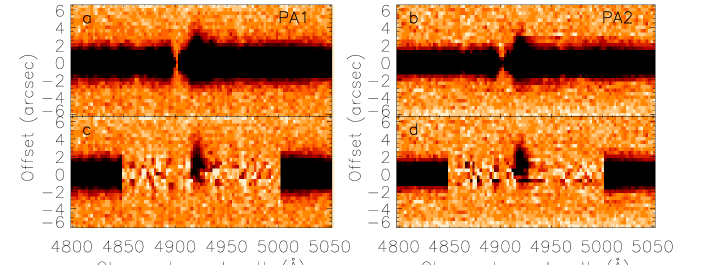
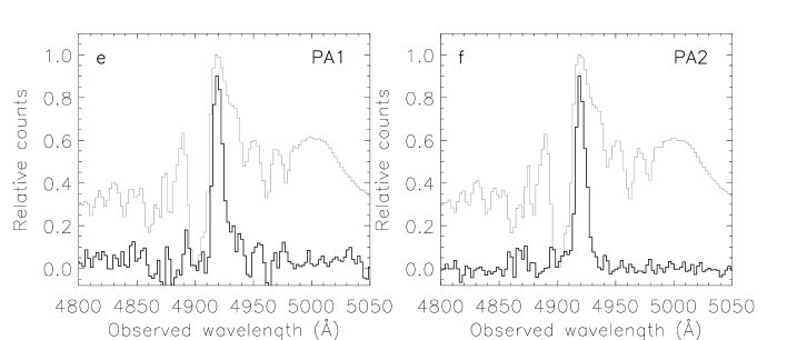
Figure 2: Spectra at PA1 (left column) and PA2 (right column). a) – b) The 2D quasar spectrum. c) – d) The 2D quasar spectrum has been subtracted between $4850$ Å and $5000$ Å revealing the extended Ly$\alpha$ emission. The zero point of the spatial axis is set to the centroid of the QSO. Note the large residuals from the quasar SPSF subtraction, which are due to the large shot noise near the centroid. e) – f) The spectrum of the QSO Ly$\alpha$ emission line (light grey curve) and the spatially averaged spectrum of the extended Ly$\alpha$ emission (black curve). The maximum flux of the extended Ly$\alpha$ emission is scaled to $90\%$ of the maximum QSO flux. The total line flux in extended Ly$\alpha$ is around $1\%$ of the flux from the QSO Ly$\alpha$ line. The overall flux scale in this plot is arbitrary.

PA1 was aligned with the two galaxies g1 and g2 (see Fig. 1) and centred on the QSO, so in this case we had to decompose the spectrum into its individual components. We employed an iterative procedure to separate the contributions from g1 and S6 to the total quasar flux: i) Extract and remove the QSO spectrum. ii) Extract and remove the spectrum of g1 and S6. The procedure converged to a stable solution after three iterations. For the PA1 observations using grism G600R the seeing conditions were slightly better than for those using G600B (see Table 1), so the projected distances of g1 and g2 were enough to bring them outside the QSO point-spread function (PSF) and we could make a normal extraction of the quasar spectrum.

Figure 3: Extracted spectrum of Q1205-30. The most prominent emission lines are indicated. The spectrum has not been extinction corrected nor flux calibrated.

Figure 4: Surface brightness and velocity profiles of the extended Ly$\alpha$ emission based on spectra at PA1 (left column) and PA2 (right column). a) – b) Surface brightness profile. The error bars are based on photon statistics only. Systematic errors due to the flux calibration are not considered. The thick dashed line shows our $5\sigma$ detection limit. c) – d) Velocity profile of the extended Ly$\alpha$ emission measured relative to the systemic redshift of the quasar (see Sect. 3.2). The uncertainties are statistical uncertainties on the position of the maximum of a fitted Gauss curve (Landman et al. 1982). In both PAs the most distant detection was too faint to allow a secure determination of the velocity. A rest-frame velocity of $600$ km s^-1 relative to the systemic quasar redshift (see Sect. 3.2) corresponds to a redshift $z=3.049$.

In the PA2 spectra we had only the QSO and S6 on the slit. In order to make sure that the extended flux of S6 was not modifying the quasar SPSF, we here used an option in the code which allowed us to exclude a wavelength region from the construction of the quasar SPSF. In the region from 4902 Å to 4987 Å the code therefore only fitted and extracted the QSO spectrum, it did not update the SPSF lookup table (for details see Møller 2000). For the general problem of decomposing a 2D spectrum of two superimposed objects there is a certain degeneracy of solutions. One may choose to assign the maximum amount of flux to one object, to the other object, or to aim for somewhere in between. In this case we decided to opt for a solution in between, which avoids digging a hole in the extended Ly$\alpha$ emission near the QSO centroid. The degeneracy has no consequence at distances larger than 1 arcsec from the QSO, but closer to the QSO the Ly$\alpha$ surface brightness of S6 is very uncertain.

The output from the code is the optimally extracted 1D and 2D spectrum of the QSO as well as the 2D spectrum of the extended Ly$\alpha$ emission. The 2D spectrum of the extended Ly$\alpha$ emission and the 1D spectrum of the QSO (with cosmic ray hits removed) are shown in Fig. 2a-2d and Fig. 3, respectively. For comparison we show a zoom of the Ly$\alpha$ emission of the quasar and the spatially averaged extended Ly$\alpha$ emission in Fig. 2e-2f.

2.3 Wavelength and flux calibrations

The spectra in Fig. 2 were wavelength calibrated using the dispcor task in IRAF. The RMS of the deviations from a 4.^th order Chebychev polynomial fit to 12-19 lines were $0.6$ Å for the G600B spectra and $0.08-0.16$ Å for 28-33 lines in the G600R spectra.

The flux calibration was done as follows. First we estimated the continuum of the QSO away from the emission lines. We divided the spectrum by the continuum, obtaining a flat spectrum, and forced it onto an arbitrary power-law. Measuring the Bessel $B-I$ colour on the resulting spectrum and comparing to the observed $B-I$ colour (Paper I) we calculated the slope of the power-law which would bring the two in agreement ($\alpha=0.65$). We then forced the spectrum onto this power and normalized it to agree with our photometric measurements. The advantage of this procedure is that to the first several orders all absolute and differential slit losses as well as atmospheric absorption are automatically taken into account for all point source objects on the slit. We estimate the absolute flux calibration to be correct to within $10\%$ while the relative is better. This applies to point sources, but not to extended sources for which there are additional slit losses. We present surface brightness profiles and rest-frame velocity curves of the extended Ly$\alpha$ emission (relative to the systemic redshift of the quasar, see Sect. 3.2) in Fig. 4.

3 Results

3.1 Redshifts of the galaxies g1 and g2

The primary purpose of this study is to clarify the nature of the extended Ly$\alpha$ emission at $z\approx 3.04$. As pointed out in Paper I the galaxies g1 and in particular g2 may have a lensing effect, enhancing and stretching the Ly$\alpha$ patch. Therefore we first set out to determine their redshifts.

We identify four emission lines in the spectrum of the blue galaxy g1. The AB-magnitudes of g1 are $B(AB)=24.8$, $I(AB)=23.3$, $n(AB)=24.1$ (Paper I). Disregarding the weak and noisy O iii $\lambda 4960$ line, we derive a mean redshift of $z=0.4732\pm 0.00011$ (Table 2). In the 2D spectrum (Fig. 5) we see along the slit a tilt of the emission lines caused by the rotation of g1. The $\lambda 4960$ line is too weak, but for the three remaining lines O ii $\lambda 3727$, H$\beta$, and O iii $\lambda 5007$, we mapped out their rotation profiles. The three profiles are identical within the errors, so we combined the profiles and performed a joint fit (see Fig. 6). From linear extrapolation of the rotation profile down to the position of the QSO ($b=0$ kpc), we find that g1 would cross the QSO spectrum at $-212\pm 20$ km s^-1 corresponding to $z=0.4722\pm 0.0001$. Assuming instead a flattened rotation curve after the observed point closest to the QSO, we find that g1 would cross the QSO spectrum at $-100\pm 10$ km s^-1 corresponding to $z=0.4727\pm 0.0001$. We shall return to a search for absorption at this redshift in Sect. 4.

Table 2: Emission lines of g1.

Line	$\lambda_{\rm vac}$	$z_{\rm em}$
	(Å)
O ii $\lambda 3727$	$5492.21$	$0.4733(5)$
H$\beta$ $\lambda 4862$	$7163.67$	$0.4731(9)$
O iii $\lambda 4960$	$7308.07$	$0.4733(2)$
O iii $\lambda 5007$	$7377.66$	$0.4731(1)$

The red galaxy g2 has no emission but absorption lines (see Fig. 7). The AB-magnitudes of g2 are $B(AB)>26.5$, $I(AB)=22.22$, $n(AB)>24.8$ (Paper I). It was suggested in Paper I that g2 most likely is a normal elliptical galaxy at $z\gtrsim 0.5$. Minimum-$\chi^{2}$ fitting to redshifted template elliptical galaxy spectra (Kinney et al. 1996) gave a best fit redshift of $z=0.865\pm 0.003$, confirming the prediction of Paper I. The observed spectrum and the best-fit template are shown in Fig. 7. The observed I-band magnitude of g2 corresponds roughly to an absolute B-band magnitude of $M_{B}=-22.1$, which is $0.7$ mag brighter than $M_{B}^{*}$ for field galaxies in the redshift interval $0.75<z<1.0$ (Cross et al. 2004)

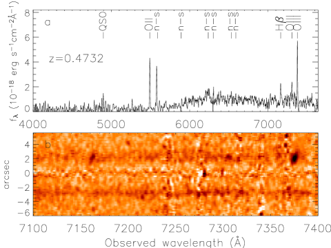
Figure 5: a) Spectrum of the blue galaxy g1 smoothed with a $7$ Å wide boxcar filter. The identified lines are indicated, and strong residuals from night sky lines are marked “n–s”. b) 2D spectrum of the QSO residuals (at $0$ arcsec), the blue galaxy g1 (at $2.12$ arcsec), and the red galaxy g2 (at $-2.77$ arcsec). The rotation profile of g1 is clearly visible in the emission lines H$\beta$ at 7162 Å and O iii at 7376 Å.

Figure 6: Rotation profile of galaxy g1 mapped out from the O ii $\lambda 3727$ ($\square$), H$\beta\leavevmode\nobreak\ \lambda 4862$ ($\diamond$) and O iii $\lambda 5007$ ($\times$) lines. The straight line is the best combined fit to all velocity profiles. The $x$-axis denotes the distance from the QSO in arcsec (bottom) and kpc (top), whereas the $y$-axis is the velocity relative to the redshift of O iii $\lambda 5007$ ($z=0.47311$).

Figure 7: Spectrum of g2 (thin line) smoothed with a $35$ Å wide boxcar filter, and template of an elliptical galaxy (thick line) at $z=0.865$ (Kinney et al. 1996). Strong residuals from night sky lines are marked “n–s”.

3.2 The systemic redshift of the QSO

The quasar spectrum contains a Lyman-limit system (LLS) very close to the redshift of the quasar (Lanzetta et al. 1991). In order to establish the relation between the QSO, the LLS and the extended Ly$\alpha$ emission we need to determine the precise redshifts of all three. For QSOs this is not entirely straight forward. It is well known that high-ionization lines are blueshifted with respect to the QSO systemic redshift by typically several hundred km s^-1 (e.g. Tytler & Fan 1992). For low-ionization lines the blueshifts are known to be small or zero.

We measure equivalent widths, line fluxes and vacuum-corrected wavelengths for eight both high- and low-ionization emission lines in the quasar spectrum after removing absorption lines from intervening systems. The results are presented in Table 3. Because the LLS redshift is very close to the QSO redshift, the quasar Ly$\alpha$ emission line is heavily absorbed, so the observed centre wavelength is dependent on how the line is reconstructed, resulting in an uncertainty of $20$ Å. We calculate the systemic redshift of the quasar using the subset of the lines listed in Table 3 which also appear with blueshift-adjusted rest-frame wavelengths in Tytler & Fan (1992). The five lines used are N v, Si ii / O i, Si iv / O iv], C iv, and C iii]. The inverse-variance weighted average of these lines provides a final $z_{\rm QSO}=3.041\pm 0.001$.

Table 3: Measured characteristics of eight QSO emission lines. The columns show the line identification, the observed wavelength in vacuum, the equivalent widths in observers frame and rest frame, the line flux, the blueshift-adjusted rest wavelengths from Tytler & Fan (1992), and the corresponding redshift. The error associated with the placement of the continuum is included in the errors on $W_{\mathrm{obs}}$, $W_{\mathrm{rest}}$ and the line flux. The Ly$\alpha$ line is heavily absorbed, so the redshift derived from this line (shown in square brackets) is not used in the calculation of the systemic QSO redshift.

Line	$\lambda_{\rm rest}$a	$\lambda_{\mathrm{vac}}$	$W_{\mathrm{obs}}$	$W_{\mathrm{rest}}$	Line flux	$\lambda_{\rm TF}$	$z_{\rm TF}$
	(Å)	(Å)	(Å)	(Å)	$(10^{-16}$ erg s-1 cm${}^{-2})$	(Å)
Ly$\alpha$	$1215.67$	$4918\pm 20$	$281\pm 15$	$69\pm 4$	$541\pm 33$	$1214.97\pm 0.07$	[$3.048\pm 0.016$]
N v	$1240.15$	$5005\pm 5$	$96\pm 4$	$24\pm 1.0$	$183\pm 27$	$1239.16\pm 0.28$	$3.039\pm 0.004$
Si ii	$1263.31$	$5101\pm 7$	$6\pm 2$	$1.5\pm 0.5$	$10\pm 3$	—	—
Si ii / O i	$1305.57$	$5281\pm 7$	$15\pm 2$	$3.8\pm 0.6$	$22.7\pm 1.5$	$1304.24\pm 0.30$	$3.049\pm 0.005$
C ii	$1335.31$	$5400\pm 3$	$9\pm 2$	$2.2\pm 0.5$	$11\pm 2$	—	—
Si iv / O iv]	$1399.55$	$5647\pm 3$	$62\pm 9$	$15\pm 2$	$81\pm 4$	$1398.62\pm 0.19$	$3.037\pm 0.002$
C iv	$1549.05$	$6249\pm 5$	$180\pm 15$	$44\pm 4$	$195\pm 11$	$1547.46\pm 0.04$	$3.038\pm 0.003$
C iii]	$1908.73$	$7722\pm 7$	$100\pm 12$	$25\pm 3$	$94\pm 9$	$1906.53\pm 0.09$	$3.050\pm 0.004$

^a Taken from Wilkes (2000).

3.3 Absorption line systems

In the quasar spectrum we identify 12 C iv absorption systems between the Ly$\alpha$ and C iv emission lines. In Fig. 8 we plot this section of the QSO spectrum normalized to the continuum. The line identifications are presented in Table 4, and the redshifts and identified lines for the 12 systems are summarized in Table 5. We expect to detect $5.2\pm 1$ C iv absorbers per unit redshift (Fig. 5 in Sargent et al. 1988). We find $13.9$ systems per unit redshift between the Ly$\alpha$ ($z=2.17$) and C iv ($z=3.04$) lines of the QSO. Applying the same selection criteria as the S2 sample of Sargent et al., namely rest equivalent widths $W_{\rm rest}>0.15$ Å for both lines in the C iv doublet, a rest-frame velocity relative to the QSO $v<-5000$ km s^-1 (in this case corresponding to $z_{\rm abs}<2.974$), and grouping systems separated by less than $1000$ km s^-1, we are left with $5.8\pm 2.4$ systems per unit redshift. Using these criteria Sargent et al. find $2.2^{+0.7}_{-0.5}$ systems per unit redshift at $z=2-3$ (Fig. 6 in Sargent et al. 1988). Our result is higher than normally observed, but still marginally consistent with the Sargent et al. study.

Table 4: Identified absorption lines redwards of Ly$\alpha$. The columns show the line number, the observed wavelength in vacuum, the observed equivalent width, the inferred redshift and the absorption line and system identification. The error bars are $1\sigma$ errors due to read-out noise and photon statistics only. The error associated with the position of the continuum is not considered. The line numbers refer to the numbering in Fig. 8.

#	$\lambda_{\rm vac}$	$W_{\rm obs}$	$z_{\rm abs}$	Identification
	(Å)	(Å)
1	$4945.0$	$1.92\pm 0.02$	$2.9917$	N v	I
2	$4963.0$	$3.82\pm 0.02$	$2.9934/3.0063$	N v	I / J
3	$4979.4$	$2.16\pm 0.02$	$3.0066$	N v	J
4	$4989.6$	$0.18\pm 0.02$	$2.8318$	O i	E
5	$4996.8$	$0.03\pm 0.02$	$2.8308$	Si ii	E
6	$5067.6$	$0.83\pm 0.03$	$2.2732$	C iv	A
7	$5075.7$	$0.57\pm 0.02$	$2.2730$	C iv	A
8	$5083.5$	$1.02\pm 0.03$	$3.0332$	Si ii	K
9	$5110.4$	$0.20\pm 0.02$	$2.8293$	C ii	E
10	$5118.5$	$0.73\pm 0.03$	$2.6725$	Si iv	D
11	$5134.1$	$0.20\pm 0.03$	$2.9427$	O i	G
12	$5142.2$	$0.10\pm 0.02$	$2.9423$	Si ii	G
13	$5152.5$	$0.50\pm 0.04$	$2.6731$	Si iv	D
14	$5187.2$	$0.07\pm 0.03$	$2.8869$	C ii	F
15	$5195.0$	$0.04\pm 0.02$	$2.9895$	O i	I
16	$5201.9$	$0.01\pm 0.02$	$2.9880$	Si ii	I
17	$5215.3$	$0.06\pm 0.03$	$3.0051$	O i	J
18	$5251.8$	$0.40\pm 0.03$	$3.0331$	O i	K
19	$5261.6$	$0.05\pm 0.03$	$2.9426$ / $3.0338$	C ii / Si ii	G / K
20	$5338.7$	$0.23\pm 0.03$	$2.8305$	Si iv	E
21	$5347.0$	$1.48\pm 0.03$	$2.4537$	C iv	B
22	$5356.1$	$0.97\pm 0.03$	$2.4538$	C iv	B
23	$5373.3$	$0.13\pm 0.03$	$2.8305$	Si iv	E
24	$5382.5$	$0.97\pm 0.03$	$3.0332$	C ii	K
25	$5414.5$	$0.04\pm 0.02$	$2.8848$	Si iv	F
26	$5448.5$	$0.07\pm 0.03$	$2.8841$	Si iv	F
27	$5495.2$	$0.34\pm 0.03$	$2.9427$	Si iv	G
28	$5531.5$	$0.29\pm 0.03$	$2.9433$	Si iv	G
29	$5563.2$	$0.22\pm 0.03$	$2.9915$	Si iv	I
30	$5577.1$	$0.28\pm 0.05$	$2.6023$	C iv	C
31	$5587.2$	$0.13\pm 0.02$	$2.6028$	C iv	C
32	$5621.7$	$1.05\pm 0.03$	$3.0335$	Si iv	K
33	$5657.9$	$0.63\pm 0.02$	$3.0334$	Si iv	K
34	$5686.9$	$2.29\pm 0.02$	$2.6732$	C iv	D
35	$5696.4$	$1.41\pm 0.02$	$2.6732$	C iv	D
36	$5932.1$	$0.58\pm 0.02$	$2.8316$	C iv	E
37	$5942.5$	$0.43\pm 0.03$	$2.8320$	C iv	E
38	$6015.8$	$0.92\pm 0.02$	$2.8857$	C iv	F
39	$6025.8$	$0.49\pm 0.02$	$2.8857$	C iv	F
40	$6103.9$	$1.69\pm 0.02$	$2.9425$	C iv	G
41	$6114.8$	$1.12\pm 0.02$	$2.9430$	C iv	G
42	$6137.3$	$1.19\pm 0.02$	$2.9641$	C iv	H
43	$6146.9$	$1.01\pm 0.33$	$2.9637$	C iv	H
44	$6159.3$	$0.36\pm 0.02$	$3.0344$	Si ii	K
45	$6165.9$	$0.10\pm 0.02$	$2.8334$	Fe ii	E
46	$6180.0$	$1.41\pm 0.02$	$2.9918$	C iv	I
47	$6190.2$	$0.97\pm 0.02$	$2.9917$	C iv	I
48	$6205.3$	$2.52\pm 0.02$	$3.0081$	C iv	J
49	$6215.7$	$2.20\pm 0.02$	$3.0081$	C iv	J
50	$6245.2$	$1.55\pm 0.01$	$3.0338$	C iv	K
51	$6256.0$	$1.47\pm 0.01$	$3.0341$	C iv	K
52	$6267.3$	$0.29\pm 0.01$	$3.0481$	C iv	L
53	$6278.8$	$0.08\pm 0.01$	$3.0488$	C iv	L

Figure 8: Zoom on the normalized spectrum of Q1205-30 between the Ly$\alpha$ and C iv QSO emission lines. The numbering of the absorption lines correspond to the numbering in Table 4.

Table 5: Overview of the absorption systems in the spectrum of Q1205-30.

System	Detected lines	$z_{\rm abs}$
A	C iv $\lambda\lambda 1548$, $1550$	$2.2731\pm 0.0001$
B	C iv $\lambda\lambda 1548$, $1550$	$2.4538\pm 0.0001$
C	C iv $\lambda\lambda 1548$, $1550$	$2.6026\pm 0.0004$
D	Si iv $\lambda\lambda 1393$, $1402$, C iv $\lambda\lambda 1548$, $1550$	$2.6730\pm 0.0004$
E	O i $\lambda 1302$, Si ii $\lambda 1304$, C ii $\lambda 1334$, Si iv $\lambda\lambda 1393$, $1402$, C iv $\lambda\lambda 1548$, $1550$, Fe ii $\lambda 1608$	$2.8309\pm 0.0009$
F	C ii $\lambda 1334$, Si iv $\lambda\lambda 1393$, $1402$, C iv $\lambda\lambda 1548$, $1550$	$2.885\pm 0.001$
G	O i $\lambda 1302$, Si ii $\lambda 1304$, C ii $\lambda 1334$, Si iv $\lambda\lambda 1393$, $1402$, C iv $\lambda\lambda 1548$, $1550$	$2.9427\pm 0.0003$
H	C iv $\lambda\lambda 1548$, $1550$	$2.9639\pm 0.0003$
I	N v $\lambda\lambda 1238$, $1242$, O i $\lambda 1302$, Si ii $\lambda 1304$, Si iv $\lambda 1393^{a}$, C iv $\lambda\lambda 1548$, $1550$	$2.991\pm 0.002$
J	O i $\lambda 1302$, N v $\lambda\lambda 1238$, $1242$, C iv $\lambda\lambda 1548$, $1550$	$3.007\pm 0.001$
K	Si ii $\lambda\lambda 1260$, $1304$, $1526$, O i $\lambda 1302$, C ii $\lambda 1334$, Si iv $\lambda\lambda 1393$, $1402$, C iv $\lambda\lambda 1548$, $1550$	$3.0336\pm 0.0004$
L	C iv $\lambda\lambda 1548$, $1550$	$3.0485\pm 0.0005$

^a Si iv $\lambda 1403$ was too weak to be detected.

The LLS at $z\approx 3.034$, which was the original target (Paper I), is identical to the absorption system K, for which both low- and high-ionization lines are detected. This is in agreement with the findings for other $z_{\rm abs}\approx z_{\rm em}$ absorbers (Savaglio et al. 1994; Hamann 1997; Møller et al. 1998). By fitting line profiles to the Ly$\alpha$ and Ly$\beta$ lines we find the H i column density to be in the interval $17\leq\log N_{{H\textsc{i}}}\leq 19.9$. The best fit gives $\log N_{{H\textsc{i}}}=19.5$. In Fig. 9 we plot the absorption lines originating from system K in velocity space relative to the redshift obtained from the O i absorption line, $z_{\rm OI}=3.0331\pm 0.0002$. We notice that high-ionization lines have systematically higher redshifts than low-ionization lines. We use the redshift from the O i line as the redshift of the low-ionization region, and we take the redshift obtained from the C iv doublet, $z_{\rm CIV}=3.0340\pm 0.0002$, to be the redshift of the high-ionization region. We find that the region of highly ionized elements moves with a velocity of $\sim 60$ km s^-1 relative to the low-ionization region. Furthermore, we notice an H i absorption system in the red wing of both the Ly$\alpha$ and Ly$\beta$ lines of the LLS (see Fig. 9). This system, which we will call system K1, has a redshift of $3.039\pm 0.002$, and we find no associated metal-lines.

We detect high-ionization N v absorption for the systems I and J. If the high degree of ionization is caused by the high UV flux from the quasar, the systems must be located between the QSO and the LLS at $z\approx 3.034$, since no UV photons pass through the LLS. The redshifts of systems I and J are lower than that of the LLS (system K), which suggests that systems I and J are high-velocity clouds. Furthermore, the high degree of ionization suggests that they are associated with the QSO. The apparent line-locking between N v $\lambda 1242$ of system I and N v $\lambda 1238$ of system J strengthens this hypothesis. The line-locking effect is thought to occur in clouds driven by radiation pressure and accelerated via absorption until the wavelength of the feature falls in the shadow of another line in a neighbouring cloud (Vilkoviskij et al. 1999; Srianand et al. 2002). The velocities of the absorption systems are $-4050$ km s^-1 (system I) and $-2850$ km s^-1 (system J) relative to the systemic redshift of the quasar.

Figure 9: Velocities of lines originating from absorption system K (the LLS) relative to $z_{\rm OI}=3.0331$. The model plotted for Ly$\alpha$ and Ly$\beta$ has an H i column density of $\log N_{{H\textsc{i}}}=19.5$. The Si ii $\lambda 1304$ transition is not included here due to the probable blend with C ii $\lambda 1334$ at $z=2.9426$ (see Table 4).

4 Foreground galaxies

A classical way to search for galaxies at intermediate or high redshifts has been to look for absorption systems in the spectra of background QSOs (e.g. Weymann et al. 1979). Studies of the galaxy counterparts of Mg ii absorption systems have concluded that the galaxies responsible for the absorption are bright galaxies which can be found at impact parameters of $\sim 100$ kpc (Bergeron & Boissé 1991, Guillemin & Bergeron 1997). Using a sample of damped Ly$\alpha$ absorbers (DLAs) Lanzetta et al. (1995) found that most galaxy counterparts of DLAs at $z\lesssim 1$ have gaseous haloes extending over $\sim 230$ kpc. This is in contrast to studies at high redshift ($z=2-3.5$), where Møller et al. (2002) have found that galaxy counterparts of DLAs reside at impact parameters $\sim 10$ kpc. The large impact parameters have been used to advocate a picture of galaxies surrounded by a large, homogeneous gaseous envelope which is responsible for the absorption, but doubt has arisen whether the galaxies at large projected distances are the true absorbers (Yanny & York 1992; Vreeswijk et al. 2003; Jakobsson et al. 2004).

We have looked for absorption lines in the QSO spectrum due to the foreground galaxies g1 and g2 located at impact parameters $12.6$ kpc and $21.3$ kpc, respectively. Considering the redshifts of g1 and g2, the only lines covered by our spectrum are Ca ii H and K, Mg ii $\lambda\lambda 2796$, $2804$, Mg i $\lambda 2853$ for both galaxies, as well as Fe ii $\lambda\lambda 2344$, $2374$, $2383$, $2587$, $2600$ for g2. Lines in the Lyman-forest are not well-constrained due to the large number of Ly$\alpha$ lines. We fitted and removed lines corresponding to Ly$\alpha$, Ly$\beta$ and O vi absorption from the C iv systems listed in Table 5. In the residuals we identify two absorption lines (see Fig. 10) which may be due to Mg ii at $z=0.4722$. Alternatively, they could be two Lyman-forest lines. In Table 6 we list the $2\sigma$ upper limits on the equivalent widths of the other lines.

We find no absorption lines in the QSO spectrum outside the Lyman-forest due to the two foreground galaxies g1 and g2 down to a $2\sigma$ upper limit on the equivalent widths of $\sim 90$ mÅ (rest frame), but we cannot exclude that g1 is a Mg ii absorber with equivalent width less than $\sim 1$ Å, as the lines would fall in the Lyman forest. Assuming that the g1 Mg ii doublet candidate is correctly identified, we cannot exclude that g1 is a DLA (see Fig. 24 in Rao & Turnshek 2000). Conversely, it is unlikely that g2 is a DLA system (Fig. 25 and 26 in Rao & Turnshek 2000).

Old elliptical galaxies have recently been found up to a redshift $z=1.9$ (Cimatti et al. 2004), but not much is known about the gas content in elliptical galaxies at these early times. The combination of a small impact parameter (corresponding to $21.3$ kpc) and strict upper limits on absorption for the elliptical galaxy g2 indicates that it has no significant gas column density at these radii. The redshift $z=0.865$ of g2 corresponds to a lookback time of $7.1$ Gyr.

Figure 10: Spectrum of Q1205-30 normalized to the continuum. In the spectrum we have subtracted lines corresponding to Ly$\alpha$, Ly$\beta$ and O vi absorption from the systems listed in Table 5. The dashed line shows the model of a possible Mg ii doublet from g1.

Table 6: Absorption line search in the QSO spectrum due to g1 and g2. The quoted upper limits are $2\sigma$ limits on the equivalent widths. The error associated with the placement of the continuum is taken into account for lines not in the Lyman-forest ($\lambda_{\rm obs}>4900$ Å).

	Ion	$\lambda_{\rm rest}$	$\lambda_{\rm expected}$	$W_{\rm rest}$
		(Å)	(Å)	(Å)
g1	Mg ii	$2796.4$	$4116.8$	$1.2^{a}$
	Mg ii	$2803.5$	$4127.4$	$1.1^{a}$
	Mg i	$2853.0$	$4200.1$	$<0.20$
	Ca ii	$3934.7$	$5792.8$	$<0.095$
	Ca ii	$3969.6$	$5844.0$	$<0.068$
g2	Fe ii	$2344.2$	$4372.0$	$<0.4$
	Fe ii	$2374.4$	$4428.4$	$<0.4$
	Fe ii	$2382.8$	$4443.9$	$<0.5$
	Fe ii	$2586.6$	$4824.1$	$<0.5$
	Fe ii	$2600.2$	$4849.3$	$<0.6$
	Mg ii	$2796.4$	$5215.2$	$<0.097$
	Mg ii	$2803.5$	$5228.6$	$<0.107$
	Mg i	$2853.0$	$5320.8$	$<0.059$
	Ca ii	$3934.7$	$7338.4$	$<0.089$
	Ca ii	$3969.6$	$7403.3$	$<0.073$

^a The line is in the Lyman-forest, so it may be Ly$\alpha$ at an intermediate redshift. The identification is therefore not secure.

4.1 Gravitational lensing

The position of g2 could introduce a lensing effect on S6. Knowing the true redshift of g2, we can repeat the calculation in Paper I of the radius of its Einstein ring. For easy comparison to Paper I we assume that g2 has a singular isothermal mass distribution with a velocity dispersion $\sigma=300$ km s^-1, in which case the radius of the Einstein ring is

$$\theta_{E}=4\pi\left(\frac{\sigma}{c}\right)^{2}\frac{d_{LS}}{d_{S}}=1.4\leavevmode\nobreak\ \text{arcsec}$$ (1)

(from the equation following Eq. 4.14 in Peacock 1999), where $d_{LS}$ is the lens-source angular distance and $d_{S}$ is the observer-source angular distance. Gravitational lensing will introduce stretching and distortion perpendicular to the radius vector from g2, most notably at a distance of one Einstein radius. Emission appearing within one Einstein radius of the centre of g2 (roughly corresponding to the dotted circle in the lower right part of Fig. 1) is expected to originate from the same small region. This stretching effect would result in a flat velocity profile along PA1, which is seen in Fig. 4c over a distance of up to $4$ arcsec from the QSO centre towards g2.

The fact that we only detect one lensed image of the quasar constrains the mass of g2 within a projected distance corresponding to the g2 – quasar angular distance (2.77 arcsec). Following the calculations of Le Brun et al. (2000), we may calculate a model independent upper limit on the projected mass $M^{\Sigma}_{\rm max}(<r_{\rm I})$ enclosed within a radius $r_{\rm I}=d_{L}\theta_{\rm I}=21.3$ kpc:

$$M^{\Sigma}_{\rm max}(<r_{\rm I})=\pi r_{\rm I}^{2}\Sigma_{\rm crit}=2.8\times 10^{12}M_{\odot},$$ (2)

where $\Sigma_{\rm crit}=\frac{c^{2}}{4\pi G}\frac{d_{S}}{d_{L}d_{LS}}$ is the critical surface density. This corresponds to an upper limit to the radius of the Einstein ring of $\theta_{E}<2.77$ arcsec.

Conversely, the following lower limit to the size of the Einstein ring allows us to constrain from below the projected mass. From Fig. 4c it is evident that the Einstein radius is at least $0.8$ arcsec (the constant part of the velocity profile between galaxy g2 at $\sim 2.8$ arcsec and out to the most distant measurement at $3.6$ arcsec). Thus $\theta_{E}>\theta_{\rm min}=0.8$ arcsec, and

$$M(<r_{\rm I})>M(<d_{L}\theta_{E})>\frac{\theta_{\rm min}^{2}c^{2}}{4G}\frac{d_{S}d_{L}}{d_{LS}}=2.3\times 10^{11}M_{\odot}.$$ (3)

Thus the projected mass of galaxy g2 is between $2.3\times 10^{11}M_{\odot}$ and $2.8\times 10^{12}M_{\odot}$ within a radius of $2.77$ arcsec ($21.3$ kpc). This is consistent with the super-$M_{B}^{*}$ finding of Sect. 3. In terms of velocity dispersion the range is $230\text{ km s}^{-1}<\sigma<420\text{ km s}^{-1}$, assuming a singular isothermal mass distribution.

5 A model of the extended Ly$\alpha$ emission

In trying to understand the extended Ly$\alpha$ emission, we have constructed a numerical model, where the quasar lies in the centre of a large, optically thin H i cloud. This model was already prosposed in Weidinger et al. (2004; hereafter Paper II) together with the main conclusions. The details of our calculations were not included in that paper, but they will now be presented here.

The quasar emission is collimated in a cone with a full opening angle $\Psi$, and the system is seen under an inclination angle $\theta$ (see Fig. 3a of Paper II). The H i within the cone is photoionized by the quasar UV photons, causing it to emit Ly$\alpha$ photons when recombining. For the calculation of the extended Ly$\alpha$-emission, we follow the treatment of the optically thin case given in Gould & Weinberg (1996). The ionization rate of a hydrogen atom at a distance $r$ from the quasar is

$$\Gamma(r)=\int_{\nu_{L}}^{\infty}\phi(\nu)\sigma(\nu)d\nu,$$ (4)

where $\phi(\nu)$ is the photon flux density

$$\phi(\nu)=\frac{f_{\nu}(r)}{h\nu}$$ (5)

and the H i ionization cross section is

$$\sigma(\nu)\approx 6.3\times 10^{-18}\text{ cm}^{2}\left(\frac{\nu}{\nu_{L}}\right)^{-2.75}.$$ (6)

Here $h\nu_{L}=13.6$ eV is the hydrogen ionization potential, and $f_{\nu}(r)$ is the frequency-specific flux at a distance $r$ from the QSO. The production rate of Ly$\alpha$ photons per unit volume is

$$\dot{n}_{{\rm Ly}\alpha}(r)=\eta_{\rm thin}n_{{H\textsc{i}}}(r)\Gamma(r),$$ (7)

where $\eta_{\rm thin}=0.42$ is the fraction of recombinations that result in a Ly$\alpha$ photon. We assume a power-law hydrogen density profile, $n_{{H\textsc{i}}}(r)=n_{{{H\textsc{i}}},1}\left(\frac{r}{1\text{ kpc}}\right)^{-\gamma}$. By integrating along the line of sight, $l$, we obtain the surface brightness (in erg s^-1 cm^-2 arcsec^-2)

$$\Sigma_{{\rm Ly}\alpha}=\frac{\int E_{{\rm Ly}\alpha}\dot{n}_{{\rm Ly}\alpha}(r)dl}{4\pi D_{L}^{2}}\frac{D_{A}^{2}}{d\Omega}.$$ (8)

Here $E_{{\rm Ly}\alpha}=10.4$ eV is the energy of a Ly$\alpha$ photon, and $D_{L}$ the quasar luminosity distance. $D_{A}$ is the angular distance, such that $\frac{d\Omega}{D_{A}^{2}}$ is the conversion from cm² to arcsec².

The flux emitted from the quasar close to the Lyman-limit frequency, $\nu_{L}$, is given by

$$f_{\nu}(r)=\begin{cases}f_{\nu_{L},\text{ obs}}\left(\frac{D_{L}}{r}\right)^{2}\left(\frac{\nu}{\nu_{L}}\right)^{-\alpha}&\text{inside the cone,}\\ 0&\text{outside the cone.}\end{cases}$$ (9)

We obtain the observed Lyman-limit flux, $f_{\nu_{L},\text{ obs}}$, using the slope of the quasar spectrum and an observed flux, $f_{\nu_{0},\text{ obs}}$, on the continuum at $\nu_{0}$, that is

$$f_{\nu_{L},\text{ obs}}=f_{\nu_{0},\text{ obs}}\left(\frac{\nu_{L}}{\nu_{0}}\right)^{-\alpha}.$$ (10)

The free parameters of the model are the observed flux at $\nu_{0}$, $f_{\nu_{0},\text{ obs}}$, the spectral slope, $\alpha$, the redshift, $z$, the angles $\Psi$ and $\theta$, the neutral hydrogen density at a distance of $1$ kpc, $n_{{{H\textsc{i}}},1}$, and the density slope, $\gamma$.

5.1 Model parameters

Several free parameters are determined directly via observations. We measure the observed continuum flux at a given point in the spectrum. For the spectral index $\alpha$ we use the value found in the flux calibration in Sect. 2.3. The obtained values for these parameters are listed in Table 7. In Paper II a method to obtain a relation between the opening angle and the inclination angle is described. The free parameters in our model are now reduced to the opening angle, $\Psi$, the hydrogen density scale, $n_{{{H\textsc{i}}},1}$, and the density slope, $\gamma$.

The numerical implementation of the model was carried out by incorporating the cone into a cubic grid inclined at an angle $\theta$. The Ly$\alpha$ production rate was calculated in each grid point within the cone, and the process of integrating along the line of sight was simply to sum along the grid $z$-axis.

Table 7: Input parameters of the model.

Description	Symbol	Value
Observed flux	$f_{\lambda_{0},\text{ obs}}$	$1.3\times 10^{-16}$ erg s-1 cm-2 Å-1
Reference wavelength	$\lambda_{0}$	$5946$ Å
Spectral slope	$\alpha$	$0.65$
Redshift	$z$	$3.041$

Figure 11: Best-fit surface brightness profiles as seen through a $1.2$ arcsec wide slit with a seeing of $0.7$ arcsec for opening angles of $90^{\circ}$ (dotted), $110^{\circ}$ (solid), $130^{\circ}$ (long dashes), $150^{\circ}$ (solid), and $170^{\circ}$ (short dashes). The model parameters are listed in Table 8. Overplotted is the measured surface brightness profile of S6 shown in Fig. 4b. Note that three marginal measurements at negative offsets are included.

Table 8: Best-fit values for $\theta$, $n_{{{H\textsc{i}}},1}$, $\gamma$, and $M_{200}$ for various opening angles.

$\Psi$	$\theta$	$n_{{{H\textsc{i}}},1}$	$\gamma$	$M_{200}$
		$(10^{-8}\text{ cm}^{-3})$		$(10^{12}M_{\odot})$
$90^{\circ}$	$22.5^{\circ}$	$9.8$	$0.018$	2.6
$110^{\circ}$	$27.2^{\circ}$	$9.3$	$0.072$	3.5
$130^{\circ}$	$31.8^{\circ}$	$8.2$	$0.093$	5.3
$150^{\circ}$	$36.5^{\circ}$	$6.4$	$0.064$	6.5
$170^{\circ}$	$41.1^{\circ}$	$5.5$	$0.054$	6.5

5.2 Results of the model

Using the parameters listed in Table 7, and assuming a given opening angle and corresponding best-fit inclination angle, we now fit the model to the observed surface brightness profile, leaving the hydrogen density scale, $n_{{{H\textsc{i}}},1}$, and slope, $\gamma$, as free parameters. The best-fit values for each opening angle are listed in Table 8, and the corresponding surface brightness profiles are plotted in Fig. 11.

The numerical model described in Paper II and above is purely geometrical. Assuming in addition that the gas is in free fall into a dark matter (DM) halo introduces a velocity field in the gas. In Paper II this was used to fit the virial mass, $M_{200}$, to the observed velocity profile. The obtained virial masses are also listed in Table 8. The conclusions are presented in Paper II.

6 Discussion

Returning to the main topic of the origin of the extended Ly$\alpha$ emission, there are several elements of this puzzle that now can to be pieced together. There is a LLS at $z=3.0336\pm 0.0004$ (absorber K, see Table 5), an additional absorber at $z=3.039\pm 0.002$ (K1, see Sect. 3.3), the systemic redshift of the quasar is $z=3.041\pm 0.001$ (Sect. 3.2), the absorber L at $z=3.0485\pm 0.0005$ (Table 5) and finally the extended Ly$\alpha$ emission S6 at $z\approx 3.049$ (see caption of Fig. 4c-d). We assume that the high-ionization, line locked systems I and J are intrinsic to the central engine and will not consider them here.

6.1 The origin of the extended Ly$\alpha$ emission

The separation of the low- and high-ionization lines in the LLS suggests that it is heated by the quasar UV photons and expanding. However, the large velocity offset between the LLS and the extended Ly$\alpha$ emission ($\sim 1000$ km s^-1) makes it very unlikely that the two are physically associated as previously thought (Paper I). Since the LLS absorbs all UV photons, the extended emission must be located between the LLS and the QSO, which makes an association between the extended Ly$\alpha$ emission and the QSO the most likely one. It was suggested by Haiman & Rees (2001) that neutral gas falling into the dark matter halo around a quasar could be photoionized by the quasar UV flux, causing the gas to emit Ly$\alpha$ photons.

Interpreting the observations in the Haiman & Rees (2001) picture as described in the numerical model (Sect. 5; Paper II), we identify K1 as absorption due to a large hydrogen cloud around the quasar, in which case the redshift of K1 should be close to that of the quasar. A part of this large cloud is pulled into the DM halo of the QSO where it is photoionized and gives rise to the Ly$\alpha$ emission of S6. S6 therefore lies between us and the quasar, and the higher redshift is due to infall. The velocity of S6 is $\sim 500$ km s^-1 relative to the quasar and the surrounding cloud (K1). The absorption system L is located somewhere between the emitting and the absorbing part of the hydrogen cloud. There are at least two possibilities for placing the LLS. i) It is very close to the quasar and moving at high velocity ($\sim-500$ km s^-1). In this case the LLS has to be very small in order for the majority of the UV photons to pass by and photoionize the surrounding hydrogen cloud. ii) The LLS is sufficiently distant for the Ly$\alpha$ photons produced in the cloud surrounding the quasar to be redshifted out of the resonance wavelength and pass through the LLS unhindered. Because the low- and high-ionization lines in the LLS are only mildly separated in velocity space ($\sim 60$ km s^-1) we favour the latter possibility.

Table 9: Redshifts, fluxes and luminosities of the Ly$\alpha$ emission from the host galaxies of radio-quiet quasars.

Quasar	$z$	Ly$\alpha$ flux	Ly$\alpha$ luminosity	Reference
		$(10^{-17}$ erg s-1 cm${}^{-2})$	$(10^{42}$ erg s${}^{-1})$
Q 0054-284	$3.616$	$6$	$7.3$	Bremer et al. (1992)
Q 0055-26	$3.656$	$8$	$10$	Bremer et al. (1992)
Q 1548+0917	$2.746$	$47$	$29$	Steidel et al. (1991)
Q 1205-30	$3.041$	$70$	$56$	This work
BR 1202-0725	$4.69$	$26$	$58$	Hu et al. (1996), Petitjean et al. (1996)

The extended Ly$\alpha$ emission could possibly be explained by other scenarios rather than the projected ionization cone. However, the combination of imaging and spectroscopic data enables us to rule out most of these other scenarios (Paper II). i) Jets are believed to be present in radio-quiet quasars. They are predicted to extend out to only $\sim 0.1$ kpc (Blundell et al. 2003), more than two orders of magnitude less than the $\sim 30$ kpc extent of the emission around Q1205-30. ii) Outflowing galactic winds are generally thought to be triggered by the cumulative effect of many supernovae exploding inside the galaxy, which would metal-enrich the outflowing gas. Around radio-loud quasars this is typically seen as extended C iv emission with strength $7-10\%$ of that of the extended Ly$\alpha$ line (Heckman et al. 1991b). Our detection limit at the position of redshifted C iv is $4\times 10^{-18}$ erg s^-1 cm^-2 arcsec^-2 ($3\sigma$), which would have enabled us to detect the typical C iv line seen around some radio-loud quasars (a strength of $10\%$ of the Ly$\alpha$ line corresponds to $7\times 10^{-18}$ erg s^-1 cm^-2 arcsec^-2). The fact that we do not detect this line makes it unlikely that it is a supernova powered outflow. The most plausible explanation that remains is cosmological infall of hydrogen.

6.2 Extending the sample

To date only a handful of detections of extended Ly$\alpha$ emission around RQQs has been reported (Steidel et al. 1991; Bremer et al. 1992; Hu et al. 1996; Petitjean et al. 1996; Bunker et al. 2003). Hu et al. (1991) find no extended Ly$\alpha$ emission in their sample of seven radio-quiet quasars down to a limiting flux of $2\times 10^{-16}$ erg s^-1 cm^-2. We have compiled a list of fluxes and luminosities for the detections of extended Ly$\alpha$ emission (see Table 9). We measure an average Ly$\alpha$ surface brightness of $\sim 7\times 10^{-17}$ erg s^-1 cm^-2 arcsec^-2 around Q1205-30. Assuming a spatial extent of $10$ arcsec², we infer a Ly$\alpha$ flux of $\sim 7\times 10^{-16}$ erg s^-1 cm^-2. The luminosity in the Ly$\alpha$ line of S6 is at the high end of the ones listed in Table 9.

It is important for the study of the link between galaxy and quasar formation to understand how frequent and under which circumstances extended Ly$\alpha$ emission arises around RQQs. The most efficient method to detect Ly$\alpha$ emission around QSOs is narrow band imaging. The study of extended Ly$\alpha$ emission can successfully be combined with narrow band searches for Ly$\alpha$ emitting (proto)-galaxies around QSOs (e.g. Fynbo et al. 2001; Fynbo et al. 2003). The follow-up multi-object spectroscopy needed to confirm candidate Ly$\alpha$ emitters may conveniently be utilized to study any extended Ly$\alpha$ emission associated with the QSO. Alternatively, integral field spectroscopy is a promising method for very detailed studies of extended emission at high redshifts (Bower et al. 2004). The method makes it possible to map out the entire velocity field of the extended emission, strongly constraining any model.

It is imperative for any search for extended Ly$\alpha$ emission around RQQs to go to very deep detection limits. Haiman & Rees (2001) predict that haloes of infalling gas around quasars should be seen in Ly$\alpha$ emission with a typical surface brightness around $10^{-18}-10^{-17}$ erg s^-1 cm^-2 arcsec^-2 and typical angular sizes between $2-3$ arcsec, i.e. with typical fluxes around $3\times 10^{-18}-7\times 10^{-17}$ erg s^-1 cm^-2. This limit has only been reached for very few surveys.

A larger sample of QSOs with extended Ly$\alpha$ emission will make it possible to address primary issues like morphology, environment, luminosity function etc. The corresponding DM halo masses obtained in a similar fashion as in Paper II may be compared to black hole masses obtained via the correlation between $M_{\rm BH}$ and quasar emission line widths (Vestergaard 2002; McLure & Jarvis 2002). A $M_{\rm DM}-M_{\rm BH}$ correlation could provide a powerful consistency check of $N$-body hydrodynamical simulations.

We are currently looking for extended Ly$\alpha$ emission in a small sample of quasars using an analysis similar to what has been employed in this paper.

- (1) Barkana, R., & Loeb, A. 2003, Nature, 421, 341
- (2) Bergeron, J., & Boissé, P. 1991, A&A, 243, 344
- (3) Blundell, K. M., Beasley, A. J., & Bicknell, G. V. 2003, ApJ, 591, L103
- (4) Bower, R. G., Morris, S. L., Bacon, R., et al. 2004, MNRAS, 351, 63
- (5) Bremer, M. N., Fabian, A. C., Sargent, W. L. W., et al. 1992, MNRAS, 258, 23
- (6) Bunker, A., Smith, J., Spinrad, H., Stern, D., & Warren, S. J. 2003, Ap&SS, 284, 357
- (7) Cimatti, A., Daddi, E., Renzini, A., et al. 2004, Nature, 430, 184
- (8) Cross, N. J. G., Bouwens, R. J., Benítez, N., et al. 2004, AJ, 128, 1990
- (9) Elvis, M. A. 2000, ApJ, 545, 63
- (10) Falomo, R., Kotilainen, J., & Treves, A. 2001, ApJ, 547, 124
- (11) Fynbo, J. P. U., Burud, I., & Møller P. 2000a, A&A, 358, 88
- (12) Fynbo, J. P. U., Ledoux, C., Møller, P., Thomsen, B., & Burud, I. 2003, A&A, 407, 147
- (13) Fynbo, J. P. U., Thomsen, B., & Møller, P. 2000b, A&A, 353, 457 (Paper I)
- (14) Fynbo, J. P. U., Møller, P., & Thomsen, B. 2001, A&A, 374, 443
- (15) Guillemin, P., & Bergeron, J. 1997, A&A, 328, 499
- (16) Gould, A., & Weinberg, D. 1996, ApJ, 468, 462
- (17) Haiman, Z., & Rees, M. J. 2001, ApJ, 556, 87
- (18) Hamann, F. 1997, ApJS, 109, 279
- (19) Heckman, T. M., Lehnert, M. D., van Breugel, W., & Miley, G. K. 1991a, ApJ, 370, 78
- (20) Heckman, T. M., Lehnert, M. D., Miley, G. K., & van Breugel, W. 1991b, ApJ, 381, 373
- (21) Hu, E. M., & Cowie, L. L. 1987, ApJ, 317, L7
- (22) Hu, E. M., Songaila, A., Cowie, L. L., & Stockton, A. 1991, ApJ, 368, 28
- (23) Hu, E. M., McMahon, R. G., & Egami, C. 1996, ApJ, 459, L53
- (24) Jakobsson, P., Hjorth, J., Fynbo, J. P. U., et al. 2004, A&A, 427, 785
- (25) Kinney, A. L., Calzette, D., Bohlin, R. C., et al. 1996, ApJ, 467, 38
- (26) Kukula, M. J., Dunlop, J. S., McLure, R. J., et al. 2001, MNRAS, 326, 1533
- (27) Landman, D. A., Roussel-Dupre, R., & Tanigawa, G. 1982, ApJ, 261, 732
- (28) Lanzetta, K. M., Bowen, D. V., Tytler, D., & Webb, J. K. 1995, ApJ, 442, 538
- (29) Lanzetta, K. M., McMahon, R. G., Wolfe, A. M., et al. 1991, ApJS, 77, 1
- (30) Lawrence, A. 1991, MNRAS, 252, 586
- (31) Le Brun, V., Smette, A., Surdej, J., & Claeskens, J.-F. 2000, A&A, 363, 837
- (32) Lehnert, M. D., Heckman, T. M., Chambers, K. C., & Miley, G. K. 1992, ApJ, 393, 68
- (33) Lehnert, M. D., van Breugel, W., Heckman, T. M., & Miley, G. K. 1999, ApJS, 124, 11
- (34) Lowenthal, J. D., Heckman, T. M., Lehnert, M. D., & Elias, J. H. 1995, ApJ, 439, 588
- (35) McLure, R. J., & Jarvis, M. J. 2002, MNRAS, 337, 109
- (36) McLure, R. J., & Jarvis, M. J. 2004, MNRAS, 353, L45
- (37) Møller, P. 2000, The ESO Messenger, 99, 31
- (38) Møller, P., Warren, S. J., & Fynbo, J. P. U. 1998, A&A, 330, 19
- (39) Møller, P., Warren, S. J., Fall, S. M., Jakobsen, P., & Fynbo, J. U. 2000, The ESO Messenger, 99, 33
- (40) Møller, P., Warren, S. J., Fall, S. M., Fynbo, J. P. U., & Jakobsen, P. 2002, ApJ, 574, 51
- (41) Navarro, J.F., Frenk, C. S., & White, S. D. M. 1997, ApJ, 490, 493
- (42) Peacock, J. A. 1999, “Cosmological Physics”, Cambridge University Press
- (43) Petitjean, P., Pécontal, E., Valls-Gabaud, D., & Charlot, S. 1996, Nature, 380, 411
- (44) Rao, S. M., & Turnshek, D. A. 2000, ApJS, 130, 1
- (45) Reuland, M., van Breugel, W., Röttgering, H., et al. 2003, ApJ, 592, 755
- (46) Ridgway, S. E., Heckman, T. M., Calzetti, D., & Lehnert, M. 2001, ApJ, 550, 122
- (47) Sánchez, S. F. & González-Serrano, J. I. 2003, A&A, 406, 435
- (48) Sargent, W. L. W., Boksenberg, A., & Steidel, C. C. 1988, ApJS, 68, 539
- (49) Savaglio, S., D’Odorico, S., & Møller, P. 1994, A&A, 281, 331
- (50) Srianand, R., Petitjean, P., Ledoux, C., & Hazard, C. 2002, MNRAS, 336, 753
- (51) Steidel, C. C., Sargent, W. L. W., & Dickinson, M. 1991, AJ, 101, 1187
- (52) Tytler, D., & Fan, X. 1992, ApJS, 79, 1
- (53) Vestergaard, M. 2002 ApJ, 571, 733
- (54) Vilkoviskij, E. Y., Efimov, S. N., Karpova, O. G., & Pavlova, L. A. 1999, MNRAS, 309, 80
- (55) Vreeswijk, P. M., Møller, P., & Fynbo, J. P. U. 2003, A&A, 409, L5
- (56) Weidinger, M., Møller, P., & Fynbo, J. P. U. 2004, Nature, 430, 999 (Paper II)
- (57) Weymann, R. J., Williams, R. E., Peterson, B. M., & Turnshek, D. A. 1979, ApJ, 234, 33
- (58) Wilkes, B. J., 2000, in: “Allen’s astrophysical quantities” (ed. Cox, A. N.), Springer Verlag
- (59) Wilman, R. J., Johnstone, R. M., & Crawford, C. S. 2000, MNRAS, 317, 9
- (60) Yanny, B., & York, D. G. 1992, ApJ, 391, 569