The Prevalence of Cooling Cores in Clusters of Galaxies at $z\approx$ 0.15–0.4

Abstract

We present a Chandra study of 38 X-ray luminous clusters of galaxies in the ROSAT Brightest Cluster Sample (BCS) that lie at moderate redshifts ($z\approx 0.15$–0.4). Based primarily on power ratios and temperature maps, we find that the majority of clusters at moderate redshift generally have smooth, relaxed morphologies with some evidence for mild substructure perhaps indicative of recent minor merger activity. Using spatially-resolved spectral analyses, we find that cool cores appear to still be common at moderate redshift. At a radius of 50 kpc, we find that at least 55 per cent of the clusters in our sample exhibit signs of mild cooling ($t_{\rm cool}<10$ Gyr), while in the central bin at least 34 per cent demonstrate signs of strong cooling ($t_{\rm cool}<2$ Gyr). These percentages are nearly identical to those found for luminous, low-redshift clusters of galaxies, indicating that there appears to be little evolution in cluster cores since $z\approx 0.4$ and suggests that heating and cooling mechanisms may already have stabilised by this epoch. Comparing the central cooling times to catalogues of central H$\alpha$ emission in BCS clusters, we find a strong correspondence between the detection of H$\alpha$ and central cooling time. We also confirm a strong correlation between the central cooling time and cluster power ratios, indicating that crude morphological measures can be used as a proxy for more rigorous analysis in the face of limited signal-to-noise data. Finally, we find that the central temperatures for our sample typically drop by no more than a factor of $\sim$3–4 from the peak cluster temperatures, similar to those of many nearby clusters.

1 Introduction

By the time a cluster of galaxies reaches a relatively relaxed state, the hot gas in the centre is likely to have a radiative cooling time which is shorter than the expected cluster age and a temperature which drops toward the centre, due to energy losses from X-ray emission (e.g., Fabian, 1994). This effect, termed a “cooling flow”, provides a mechanism by which matter can condense out of the hot intracluster medium (ICM) and is observationally detected as an enhanced X-ray surface brightness peak in the cores of clusters. The final state of this cooling gas is still a matter of intense debate (e.g., Peterson et al., 2001; Tamura et al., 2001; Peterson et al., 2003; Kaastra et al., 2004), as the temperatures of the cooling gas are found to generally drop by less than a factor of $\sim$3–4 with very little cooler gas (presumably due to some form of heating, such as from an active galactic nucleus). Despite this cooling “floor”, and the fact that the mass of gas cooling to zero represents only a tiny fraction of the overall hot phase of the ICM, cooling cores remain an observational phenomenon which inexplicably trace the physical processes by which clusters of galaxies form. In general, the central regions of a cluster of galaxies must remain relatively relaxed both to establish and maintain a cooling core. Strong disturbances to the cluster, such as might be caused by merging for example, should mix the cluster gas and could disrupt the cooling core. The extent to which the cooling core can be suppressed or destroyed, in fact, depends on a number of factors such as the initial strength of the cooling core, how off-centre the merger is, and the mass ratio of merging systems (e.g., McGlynn & Fabian, 1984; Edge, Stewart, & Fabian, 1992; Allen et al., 2001; Gómez, Loken, Roettiger, & Burns, 2002; Ritchie & Thomas, 2002). Thus, a proper census of cooling cores in clusters as a function of lookback time should provide important constraints on the robustness of cooling cores, the nature of cluster buildup and allow further refinements to structure formation models.

Central surface brightness peaks in clusters of galaxies (the observational signature of cool cores) appear to be remarkably widespread, residing in 70–90 per cent of the clusters with $z<0.10$, and occasionally even dominating their bolometric output (e.g., Edge, Stewart, & Fabian, 1992; Peres et al., 1998). The ages of these cooling cores, typically considered to be the time since their last disruption, are estimated to be $<4$ Gyr in $\sim$50 per cent of the objects (Allen & Fabian, 1997; Allen et al., 2001). By observing galaxy clusters at $z\approx 0.15$–0.4 (i.e., lookback times of 2–4 Gyr), we can probe the conditions of these objects during a potentially important disruption period. The question of how common cooling cores are in the more distant past remains completely unexplored. We report here on a large sample of moderate redshift clusters with Chanda observations. The sub-arcsecond spatial resolution afforded by Chandra is extremely important in this effort, as it allows the detection and quantification of cooling cores out to much larger distances than was previously accessible with past X-ray observatories such as Einstein and ROSAT.

We describe our X-ray sample in $\S$2, analysis of the Chandra data in $\S$3, and finally, our results in $\S$4. Throughout this paper, we adopt $H_{0}=70$ km s^-1 Mpc^-1, $\Omega_{\rm M}=0.3$, and $\Omega_{\Lambda}=0.7$. Unless explicitly stated otherwise, quoted errors are for a $1\sigma$ (68 per cent) confidence level.

2 Sample Selection

We selected our sample from the ROSAT Brightest Cluster Sample (BCS; Ebeling et al., 1998) and Extended ROSAT Brightest Cluster Sample (EBCS; Ebeling et al., 2000), both of which are derived from ROSAT All-Sky Survey data. When combined (hereafter simply BCS), they represent one of the largest and most complete X-ray-selected cluster samples compiled to date. Figure 1 highlights the fraction of BCS sources with Chandra observations, shown in the 0.1–2.4 keV luminosity versus redshift plane. Importantly, a large fraction of the most luminous and most distant BCS sources have already been observed by Chandra. We adopt a selection criterion of $z>0.15$ to maximize the average redshift of the sample, while still providing a statistically useful number of objects with Chandra observations. Of the 51 clusters with $z>0.15$, 38 (75 per cent) have publicly available Chandra exposures as of 2003 October. The vast majority of these are of sufficient quality (i.e., $\ga$5000 counts) to assess crudely the nature of any potential cooling core. Thus, our sample should be sufficiently complete to provide reliable statistics on luminous clusters of galaxies at moderate redshifts. As a local comparison sample, we use the Brightest 55 sample studied by Peres et al. (hereafter B55; 1998). The B55 sample is a 2–10 keV flux limited sample of X-ray emitting clusters which is nearly complete and comprised of sources which are all close enough to have been imaged properly with previous X-ray instruments (i.e., ROSAT). To make the B55 sample more comparable with ours, we have cropped two clusters with $z>0.15$ and excluded clusters with $L_{0.1--2.4~{}keV}<4\times 10^{44}$. We have converted the B55 values to our adopted cosmology.

Figure 1: X-ray luminosity versus redshift for the BCS sample (circles). Filled circles denote BCS clusters observed with Chandra as of 2003 October. Our sample consists of those sources with $z\geq 0.15$.

Table 1: Summary of Chandra Observations for the $z>0.15$ BCS Sample.

(1)	(2)	(3)	(4)	(5)	(6)
Cluster	ObsID	Date	ACIS	Exp.	Bgd
A68	3250	2002-09-07	I	9.9	1.039
A115a	3233	2002-10-07	I	50.0	1.045
A115b	3233	2002-10-07	I	50.0	1.045
A267	1448	1999-10-16	I	7.8	1.052
A520	528	2000-10-10	I	9.3	1.010
A586	530	2000-09-05	I	9.8	1.148
A665	3586	2002-12-28	I	30.1	1.068
	531	1999-12-29	I	8.8	1.126
A697	4217	2002-12-15	I	19.7	0.955
	532	1999-10-21	I	4.4	1.765*
A750	924	2000-10-02	I	29.1	1.123
A773	533	2000-09-05	I	11.1	1.071
A781	534	2000-10-03	I	9.9	1.032
A963	903	2000-10-11	S	36.3	0.991
A1204	2205	2001-06-01	I	23.9	0.984
A1423	538	2000-07-07	I	9.5	1.019
A1682	3244	2002-10-19	I	9.6	1.784!
A1758a	2213	2001-08-28	S	58.6	1.516!
A1763	3591	2003-08-28	I	19.2	0.935
A1835	495	1999-12-11	S	19.7	1.327!
	496	2000-04-29	S	10.6	1.323*
A1914	542	1999-11-21	I	7.8	1.329!
A2111	544	2000-03-22	I	10.1	1.084
A2204	499	2000-07-29	S	10.1	1.679!
A2218	1666	2001-08-30	I	46.7	1.010
	1454	1999-10-19	I	11.4	1.245*
	553	1999-10-19	I	5.7	1.219*
A2219	896	2000-03-31	S	42.5	1.573!
A2259	3245	2002-09-16	I	9.9	0.990
A2261	550	1999-12-11	I	9.1	1.310!
A2294	3246	2001-12-24	I	9.8	1.106
A2390	500	2000-10-08	S	9.6	1.038
	501	1999-11-05	S	8.8	1.344*
Hercules A	1625	2001-07-25	S	14.8	1.167!
RXJ0439.0+0520	527	2000-08-29	I	9.6	1.003
RXJ0439.0+0715	3583	2003-01-04	I	18.7	0.948
	1449	1999-10-16	I	6.0	1.132
RXJ1532.9+3021	1649	2001-08-26	S	9.3	1.056
	1665	2001-09-06	I	9.9	1.020
RXJ1720.1+2638	4361	2002-08-19	I	25.7	0.990
	3224	2002-10-03	I	23.8	1.035
	1453	1999-10-19	I	7.8	1.291*
RXJ2129.6+0005	552	2000-10-21	I	9.9	0.942
Z1953	1659	2000-10-22	I	24.9	0.971
Z2701	3195	2001-11-04	S	27.0	1.563!
Z3146	909	2000-05-10	I	46.4	0.987
Z5247	539	2000-03-23	I	9.1	1.116
Z7160	543	2000-05-19	I	9.6	1.055

Col. 1: Cluster name. Col. 2: Chandra observation number. All observations are used for image analysis, while only the first observation is used for spectral analysis. Col. 3: Observation date. Col. 4: Whether observation was ACIS-I or ACIS-S (i.e., cluster centre was positioned on chip I3 or S3, respectively). Col. 5: Useful exposure time after the data were cleaned and background flares removed, in units of ks. Col. 6: Ratio of the average 0.3–10 keV background count rate for each observation versus the ACIS quiescent-background calibration values (i.e., 0.31 cts s^-1 per ACIS-I chip and 0.86 cts s^-1 per ACIS-S3 chip; see Sect. 3.1). Symbols indicate that the observation has a high background, but was used only for image analysis (“*”) or for both image and spectral analysis (“!”).

Table 2: General Properties of the Cool Core Sample.

(1)	(2)	(3)	(4)	(5)	(6)	(7)	(8)	(9)	(10)	(11)	(12)	(13)
Cluster	Position (J2000)	$N_{\rm H}$	$kT$	$z$	$F_{\rm X}$	$L_{\rm X}$	$H\alpha$	Mor.	$R_{\rm cent}$	$t_{\rm cool}$	$t_{\rm 50}$	$t_{\rm 180}$
A68	00h37m06$\aas@@fstack{s}$1 $+$09∘09′34″	4.6	10.0	0.2546	5.5	14.89	?	R	41.3	$24.0^{+10.6}_{-10.8}$	$24.0^{+10.6}_{-10.8}$	$57.5^{+0.0}_{-22.6}$
A115a*	00h55m50$\aas@@fstack{s}$9 $+$26∘24′35″	5.2	9.8	0.1971	9.0	14.59	Y	D	17.4	$1.6^{+0.2}_{-0.2}$	$4.0^{+0.7}_{-0.6}$	$23.0^{+5.8}_{-4.1}$
A115b*	00h55m59$\aas@@fstack{s}$4 $+$26∘20′13″	5.2	9.8	0.1971	9.0	14.59	?	D	43.1	$22.0^{+9.7}_{-6.2}$	$22.0^{+9.7}_{-6.2}$	$34.1^{+62.1}_{-10.4}$
A267	01h52m42$\aas@@fstack{s}$1 $+$01∘00′38″	2.8	9.7	0.2300	6.2	13.71	N	R	36.9	$25.1^{+4.2}_{-13.1}$	$25.1^{+4.2}_{-13.1}$	$22.0^{+20.7}_{-6.7}$
A520	04h54m09$\aas@@fstack{s}$8 $+$02∘55′16″	7.4	9.8	0.2030	8.4	14.44	N	D	52.7	$14.8^{+13.6}_{-4.8}$	$13.6^{+12.5}_{-4.4}$	$24.5^{+23.2}_{-7.8}$
A586	07h32m20$\aas@@fstack{s}$3 $+$31∘37′56″	5.4	8.7	0.1710	9.1	11.12	N	R	30.2	$8.8^{+4.3}_{-2.0}$	$8.8^{+4.3}_{-2.0}$	$15.8^{+4.3}_{-2.8}$
A665	08h30m58$\aas@@fstack{s}$0 $+$65∘50′54″	4.0	8.3	0.1818	11.8	16.33	N	D	38.4	$18.2^{+14.9}_{-5.5}$	$18.2^{+14.9}_{-5.5}$	$16.2^{+4.4}_{-3.0}$
A697	08h42m57$\aas@@fstack{s}$7 $+$36∘21′57″	3.4	10.5	0.2820	5.0	16.30	N	R	43.6	$28.4^{+5.2}_{-12.7}$	$28.4^{+5.2}_{-12.7}$	$25.3^{+21.5}_{-8.4}$
A750	09h09m12$\aas@@fstack{s}$2 $+$10∘58′36″	3.6	8.1	0.1630	8.3	9.30	N	R	22.9	$7.2^{+2.5}_{-1.6}$	$7.2^{+2.5}_{-1.6}$	$25.1^{+9.2}_{-5.5}$
A773	09h17m52$\aas@@fstack{s}$9 $+$51∘43′37″	1.5	9.4	0.2170	6.7	13.08	N	R	33.1	$24.8^{+11.6}_{-15.8}$	$24.8^{+11.6}_{-15.8}$	$63.4^{+0.0}_{-24.4}$
A781	09h20m25$\aas@@fstack{s}$4 $+$30∘30′13″	1.9	10.8	0.2984	4.7	17.22	?	2	81.7	$17.4^{+8.9}_{-4.6}$	$7.2^{+3.7}_{-1.9}$	$17.4^{+8.9}_{-4.6}$
A963	10h17m03$\aas@@fstack{s}$5 $+$39∘02′54″	1.4	8.6	0.2060	5.9	10.41	N	R	20.8	$4.5^{+0.9}_{-0.7}$	$4.5^{+0.9}_{-0.7}$	$23.1^{+6.0}_{-4.5}$
A1204	11h13m20$\aas@@fstack{s}$4 $+$17∘35′38″	1.4	7.5	0.1904	5.0	7.62	Y	R	9.5	$1.1^{+0.3}_{-0.2}$	$2.1^{+0.4}_{-0.3}$	$15.4^{+2.2}_{-1.8}$
A1423	11h57m17$\aas@@fstack{s}$2 $+$33∘36′39″	1.6	8.5	0.2130	5.3	10.03	N	R	24.4	$4.2^{+1.7}_{-1.1}$	$4.2^{+1.7}_{-1.1}$	$22.5^{+13.0}_{-6.5}$
A1682	13h06m51$\aas@@fstack{s}$8 $+$46∘33′13″	1.1	8.9	0.2260	5.3	11.26	N	2	49.4	$34.6^{+35.8}_{-18.2}$	$34.6^{+35.8}_{-18.2}$	$113.0^{+0.0}_{-48.5}$
A1758a	13h32m43$\aas@@fstack{s}$5 $+$50∘32′44″	1.1	9.1	0.2800	3.6	11.68	N	2	62.7	$31.8^{+20.5}_{-9.6}$	$21.4^{+13.8}_{-6.5}$	$38.0^{+27.0}_{-11.6}$
A1763	13h35m18$\aas@@fstack{s}$7 $+$40∘59′59″	0.9	10.0	0.2279	6.9	14.93	N	R	45.6	$13.6^{+8.9}_{-3.8}$	$13.6^{+8.9}_{-3.8}$	$36.6^{+33.4}_{-10.0}$
A1835	14h01m02$\aas@@fstack{s}$0 $+$02∘52′40″	2.2	14.8	0.2528	14.7	38.53	Y	R	11.5	$0.6^{+0.1}_{-0.1}$	$1.0^{+0.1}_{-0.1}$	$12.5^{+4.4}_{-2.4}$
A1914	14h26m00$\aas@@fstack{s}$8 $+$37∘49′37″	1.0	10.8	0.1712	15.0	18.39	N	2	29.6	$14.2^{+11.5}_{-6.5}$	$14.2^{+11.5}_{-6.5}$	$35.9^{+0.0}_{-12.4}$
A2111	15h39m41$\aas@@fstack{s}$1 $+$34∘25′10″	2.0	8.8	0.2290	5.0	10.94	N	R	50.1	$21.4^{+38.1}_{-9.5}$	$21.4^{+38.0}_{-9.5}$	$38.7^{+40.8}_{-19.8}$
A2204	16h32m47$\aas@@fstack{s}$0 $+$05∘34′32″	5.3	11.4	0.1524	21.9	21.25	Y	R	7.7	$0.3^{+0.0}_{-0.0}$	$1.4^{+0.2}_{-0.1}$	$17.9^{+4.6}_{-3.2}$
A2218	16h35m52$\aas@@fstack{s}$0 $+$66∘12′34″	3.4	6.7	0.1710	7.5	9.30	?	R	34.0	$30.9^{+10.7}_{-12.0}$	$30.9^{+10.7}_{-12.0}$	$18.4^{+3.1}_{-3.1}$
A2219	16h40m20$\aas@@fstack{s}$2 $+$46∘42′30″	1.7	11.4	0.2281	9.5	20.40	N	R	41.1	$29.1^{+0.0}_{-4.5}$	$29.1^{+0.0}_{-4.5}$	$24.9^{+10.3}_{-5.6}$
A2259	17h20m08$\aas@@fstack{s}$4 $+$27∘40′10″	3.8	7.1	0.1640	5.9	6.66	N	R	28.9	$9.0^{+6.2}_{-2.8}$	$9.0^{+6.2}_{-2.8}$	$15.3^{+8.7}_{-3.5}$
A2261	17h22m27$\aas@@fstack{s}$0 $+$32∘07′57″	3.2	10.8	0.2240	8.7	18.18	N	R	18.6	$3.0^{+1.7}_{-0.9}$	$5.0^{+2.9}_{-1.4}$	$22.3^{+23.5}_{-8.4}$
A2294	17h24m05$\aas@@fstack{s}$5 $+$85∘53′15″	6.1	7.1	0.1780	5.0	6.62	Y	R	31.8	$13.1^{+15.5}_{-4.5}$	$13.1^{+15.5}_{-4.5}$	$64.5^{+0.0}_{-17.0}$
A2390	21h53m36$\aas@@fstack{s}$9 $+$17∘41′46″	6.6	11.6	0.2329	9.6	21.44	Y	R	20.8	$1.9^{+0.4}_{-0.3}$	$1.9^{+0.4}_{-0.3}$	$11.7^{+3.4}_{-2.4}$
Hercules A	16h51m08$\aas@@fstack{s}$2 $+$04∘59′33″	6.0	6.6	0.1540	5.6	5.62	?	R	17.1	$1.3^{+0.1}_{-0.1}$	$1.3^{+0.1}_{-0.1}$	$22.4^{+6.0}_{-4.5}$
RXJ0439.0+0520	04h39m02$\aas@@fstack{s}$4 $+$05∘20′43″	9.7	7.9	0.2080	4.8	8.62	Y	R	7.8	$0.5^{+0.1}_{-0.1}$	$4.1^{+2.2}_{-1.1}$	$19.0^{+7.5}_{-4.9}$
RXJ0439.0+0715	04h39m00$\aas@@fstack{s}$5 $+$07∘16′00″	1.0	9.5	0.2443	5.3	13.25	N	R	30.6	$6.1^{+1.5}_{-1.0}$	$6.1^{+1.5}_{-1.0}$	$20.0^{+9.3}_{-5.1}$
RXJ1532.9+3021	15h32m53$\aas@@fstack{s}$8 $+$30∘20′59″	2.1	12.5	0.3615!	5.0	24.40	Y	R	10.1	$0.5^{+0.1}_{-0.1}$	$0.7^{+0.3}_{-0.1}$	$15.2^{+5.3}_{-3.8}$
RXJ1720.1+2638	17h20m10$\aas@@fstack{s}$1 $+$26∘37′29″	3.9	10.2	0.1640	14.3	16.12	Y	R	13.6	$1.9^{+0.4}_{-0.3}$	$1.9^{+0.3}_{-0.2}$	$15.2^{+2.6}_{-1.9}$
RXJ2129.6+0005	21h29m39$\aas@@fstack{s}$9 $+$00∘05′18″	4.3	11.0	0.2350	8.1	18.59	Y	R	13.1	$0.7^{+0.1}_{-0.1}$	$3.2^{+1.6}_{-0.8}$	$20.7^{+10.7}_{-5.7}$
Z1953	08h50m07$\aas@@fstack{s}$0 $+$36∘04′20″	3.1	14.5	0.3737	6.1	34.12	?	R	33.3	$28.8^{+4.6}_{-17.4}$	$28.8^{+4.6}_{-17.4}$	$23.4^{+25.7}_{-9.2}$
Z2701	09h52m49$\aas@@fstack{s}$2 $+$51∘53′05″	0.9	8.7	0.2140	5.6	10.68	Y	R	13.4	$1.2^{+0.3}_{-0.1}$	$2.9^{+0.6}_{-0.4}$	$19.2^{+4.3}_{-3.1}$
Z3146	10h23m39$\aas@@fstack{s}$6 $+$04∘11′12″	2.7	12.8	0.2906	7.7	26.47	Y	R	11.4	$0.6^{+0.0}_{-0.0}$	$1.5^{+0.2}_{-0.2}$	$12.0^{+1.9}_{-1.6}$
Z5247	12h34m21$\aas@@fstack{s}$8 $+$09∘47′03″	1.7	8.5	0.2290	4.6	10.12	N	2	95.5	$169.0^{+43.3}_{-115.4}$	$57.3^{+14.7}_{-39.1}$	$169.0^{+43.3}_{-115.4}$
Z7160	14h57m15$\aas@@fstack{s}$0 $+$22∘20′34″	3.1	9.6	0.2578	4.8	13.19	Y	R	9.3	$0.7^{+0.3}_{-0.2}$	$1.5^{+0.5}_{-0.3}$	$21.2^{+11.8}_{-5.5}$

Col. 1: Cluster name. *The ROSAT derived temperature, flux and luminosity given for A0115 were measured for the source as a whole, rather than as two separate, merging clusters; given their projected separation, we treat them as individual clusters in our analysis. Col. 2: Cluster J2000 centroid position as determined from the Chandra image after excising contaminating point sources. Col. 3: Galactic absorption column, in units of $10^{20}$ cm^-2. Col. 4: BCS temperature as derived from $L_{\rm X}$–$T$ relation, in units of keV. Col. 5: BCS redshift. Col. 6: BCS unabsorbed X-ray flux in the 0.1–2.4 keV band, in units of $10^{-12}$ erg^-1 s^-1 cm^-2 Col. 7: BCS intrinsic X-ray luminosity in the 0.1-2.4 keV band (cluster rest frame), in units of $10^{44}$ erg^-1 s. Values in columns 3–7 are taken from Ebeling et al. (1998), except for the redshift of RXJ1532.9$+$3021 denoted by “!”, which was determined more accurately by Crawford et al. (1999). Col. 8: Detection of $H\alpha$ line emission as determined by Crawford et al. (1999). Y$=$yes, N$=$no, ?$=$not observed. Col. 9: Cluster morphology. Assessed by eye. R$=$regular, D$=$Disturbed, 2$=$Double peaked, often disturbed. Col. 10: Central cooling bin radius at which the central cooling time is measured, in units of kpc. Col. 11: Central cooling time, in units of Gyr. Col. 12: Cooling time at 50 kpc, in units of Gyr. Taken from the closest bin below 50 kpc, or interpolated if the central bin is above 50 kpc. (see $\S$ 4.1 for details). Col. 13: Cooling time at 180 kpc, in units of Gyr. Taken from the closest bin below 180 kpc (see $\S$ 4.1 for details).

3 Data

3.1 Preparation

The Chandra data (see Table 1) were processed and cleaned using the CIAO software and calibration files (CIAO v3.0.2, CALDB 2.27) provided by the Chandra X-ray Center (CXC), but also with FTOOLS (v5.3.1) and custom software. We began by reprocessing the data with the CIAO tool ACIS_PROCESS_EVENTS to remove the standard pixel randomisation and to flag potential ACIS background events for data observed in Very Faint (VF) mode. The data were then corrected for the radiation damage sustained by the CCDs during the first few months of Chandra operations using the charge transfer inefficiency correction procedure of Townsley et al. (2002). Following CTI-correction, we performed standard grade selection, excluding all bad columns, bad pixels, cosmic-ray afterglows, and VF-mode background events when applicable. We used only data taken during times within the CXC-generated good-time intervals. Furthermore, light curves for each dataset were made to screen for periods of high background; periods exceeding 3$\sigma$ of the mean rate were removed.

Backgrounds rates were then estimated from local regions as free of cluster emission as possible; in a few instances where large clusters were observed with ACIS-S, our background rate estimates are likely to be contaminated upward by faint cluster emission. Ratios of the average 0.3–10 keV background count rate for each observation to that of ACIS quiescent-background calibration values (i.e., 0.31 cts s^-1 per ACIS-I chip and 0.86 cts s^-1 per ACIS-S3 chip) are listed in Table 1. The vast majority of the observations have average background rates consistent to better than 15 per cent with ACIS quiescent-background calibration measurements.

For such observations, the blank sky backgrounds of M. Markevitch, processed in an identical manner to the original sample datasets, were used to characterise the X-ray background. For the remaining observations with high background rates (noted in column 7 of Table 1 by “!” or “*”; the symbols respectively denote observations used for both imaging and spectral analysis and imaging analysis only), local backgrounds were determined from regions as free of cluster emission as possible. The sample clusters are all small enough that we easily can extract source free background regions on the I0-I3 chips for ACIS-I. However, we caution that background regions on the S3 chip for ACIS-S may still include some faint cluster emission, thereby affecting the spectral analysis for a few of the outermost regions/annuli. Note that the degree of such background contamination is thus too small to significanly bias any of our conclusions.

Observations were combined for imaging and source detection purposes, using the 0.3–7.0 keV band. Contaminating point sources were found using WAVDETECT and masked out of the event lists using their 95 per cent encircled-energy radii e.g., Feigelson, Broos, & Gaffney 2000; Jerius et al., 2000; M. Karovska and P. Zhao 2001, private communication. Cluster centres were determined using a simple centroiding method on the masked 0.3–7.0 keV X-ray images (these are given in Table 2). Radial profiles for each cluster were fit initially with single 1-D beta models, followed by double 1-D beta models if the fit resulted in a $\chi^{2}_{\nu}>2.0$. The core radius, beta index, and amplitude were allowed to vary over sensible limits. Postage stamp 0.3–7.0 keV X-ray images and radial profiles for each cluster are provided in Figure 2.

Figure 2: $\star$Images are too large to include in astro-ph version; download full version at http://www.astro.columbia.edu/ feb/Bauer.ps.gz Left: $8\arcmin\times 8\arcmin$ colour images for each BCS cluster in the sample with Chandra data, comprised from the 0.5–1.0 keV (red), 1–2 keV (green), and 2–7 keV (blue) X-ray energy bands. The images have been spatially binned by a factor of 2, smoothed with a $\sigma=$3 pixel Gaussian smoothing scale, and logarithmically scaled (following the methods of Lupton et al., 2004). The white cross denotes the cluster centroid, while the white circle indicates a radius of 0.5 Mpc at the distance of each cluster. Middle: Radial profiles for each BCS cluster in the sample. Right: Projected temperature maps for each BCS cluster in the sample, scaled between 0–20 keV. The maps have been cropped to the 0.5 Mpc radius shown in the colour images to speed computation. The signal-to-noise of the data in each region (which varies between 20–40) is shown in the bottom right corner of each map.

From inspection of the postage stamp images and radial profiles in Figure 2, the majority of the clusters appear relatively regular and relaxed, although a notable minority exhibit clear asymmetric morphologies suggestive of recent merger activity or sharp discontinuities indicative of inhomogeneities (e.g., cold fronts or shocks). We calculated power ratios for each cluster to quantify obvious morphological structure within the sample in an objective manner.

3.2 Power Ratios

Power ratios allow comparisons of cluster morphologies on a common scale, effectively normalising cluster fluxes within a specified aperture. Following the prescription in Buote & Tsai (1996), we determined power ratios for each of the 38 clusters in the sample. As described therein, the power ratios are derived from the multipole expansion of the two-dimensional gravitational potential owing to matter interior to a user-defined aperture, essentially measuring the square of the ratio of higher order multipole moments to the monopole moment (i.e., $P_{1}/P_{0}$, $P_{2}/P_{0}$, $P_{3}/P_{0}$…). The coordinate system is chosen such that $P_{1}$ is trivially zero, and thus the power ratios $P_{2}/P_{0}$, $P_{3}/P_{0}$, and $P_{4}/P_{0}$ provide the most useful information for elucidating basic morphological/evolutionary trends (Buote & Tsai, 1996, e.g.,). Low values of $P_{m}/P_{0}$ indicate highly relaxed, compact and symmetric clusters on the scale of the aperture used, while high values indicate either relatively flat, spread out clusters or clusters with significant substructure or disturbed morphologies. Odd multipole ratios yield the largest differences between single and bimodal clusters, essentially vanishing for single-component clusters. $P_{3}/P_{0}$ is particularly sensitive to unequal-sized bimodals, with higher values for stronger bimodal asymmetry. Even multipole ratios are also able to separate bimodals from low-ellipticity single-component clusters, but demonstrate more considerable overlap between flatter single-component clusters and moderately bimodal clusters than the odd terms.

The power ratios for the 38 BCS clusters are plotted in Figure 3, as well as listed in Table 3. We used intrinsic physical apertures of 0.5 Mpc to allow comparisons with more nearby cluster samples. Images were normalized by 0.3–7.0 keV exposure maps and the average background values listed in Table 1 were subtracted off. Errors were determined through 1000 Monte Carlo simulations whereby we added Poisson noise to each cluster image and recalculated power ratios. As zero is a very poor estimate of the Poisson noise, we instead adopted the average background value per pixel (typically quite small) for each empty pixel of a given observation.

We find that the power ratios from this sample occupy nearly identical parameter space to those from the nearby sample of clusters from Buote & Tsai (1996). The only deviations are from the extremely compact clusters A0115a, A2294, and RXJ0439.0$+$0520 which extend to very low $P_{2}/P_{0}$ values. Overall, the majority of clusters in our sample lie in the region of power ratio parameter space typical of relaxed, symmetric clusters.

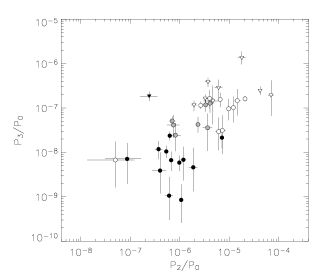
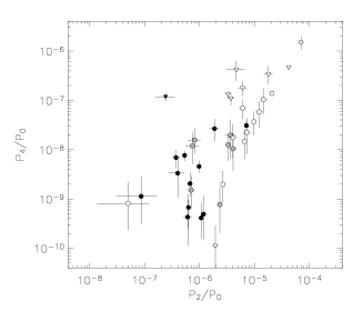
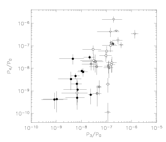
Figure 3: Power ratios for the 38 BCS clusters in the sample using a 0.5 Mpc aperture. Filled black, grey, and empty symbols denote clusters with strong cool cores ($t_{c}<2$ Gyr), weak cool cores ($t_{c}=2$–10 Gyr), and no obvious cool cores ($t_{c}>10$ Gyr), respectively. Circles denote morphologically regular clusters, while triangles denote double-peaked or disturbed clusters. A2294 (open circle in the lower left of the first two panels) is again an exception, being a very compact cluster without a cool core.

Table 3: Power Ratios for the Cool Core Sample.

(1)	(2)	(3)	(4)
Cluster	$P_{2}/P_{0}$	$P_{3}/P_{0}$	$P_{4}/P_{0}$
A68	$(1.21^{+0.17}_{-0.14})\times 10^{-5}$	$(1.02^{+0.80}_{-0.55})\times 10^{-7}$	$(5.80^{+3.94}_{-2.99})\times 10^{-8}$
A115a	$(2.40^{+1.12}_{-0.83})\times 10^{-7}$	$(1.86^{+0.48}_{-0.41})\times 10^{-7}$	$(1.18^{+0.24}_{-0.21})\times 10^{-7}$
A115b	$(3.72^{+0.52}_{-0.51})\times 10^{-6}$	$(3.87^{+0.91}_{-0.91})\times 10^{-7}$	$(1.09^{+0.34}_{-0.30})\times 10^{-7}$
A267	$(7.23^{+1.17}_{-1.11})\times 10^{-6}$	$(3.14^{+3.75}_{-2.22})\times 10^{-8}$	$(2.25^{+2.09}_{-1.44})\times 10^{-8}$
A520	$(6.08^{+1.14}_{-1.04})\times 10^{-6}$	$(2.88^{+1.47}_{-1.18})\times 10^{-7}$	$(1.76^{+0.65}_{-0.56})\times 10^{-7}$
A586	$(8.18^{+2.25}_{-2.10})\times 10^{-7}$	$(2.45^{+2.17}_{-1.39})\times 10^{-8}$	$(1.56^{+1.18}_{-0.74})\times 10^{-8}$
A665	$(3.27^{+0.32}_{-0.27})\times 10^{-6}$	$(1.64^{+0.35}_{-0.33})\times 10^{-7}$	$(1.33^{+0.21}_{-0.20})\times 10^{-7}$
A697	$(6.55^{+0.71}_{-0.69})\times 10^{-6}$	$(1.56^{+0.64}_{-0.51})\times 10^{-7}$	$(1.47^{+1.12}_{-0.83})\times 10^{-8}$
A750	$(2.33^{+0.28}_{-0.25})\times 10^{-6}$	$(4.25^{+2.03}_{-1.47})\times 10^{-8}$	$(7.68^{+9.99}_{-5.63})\times 10^{-10}$
A773	$(6.11^{+0.87}_{-0.83})\times 10^{-6}$	$(2.94^{+3.19}_{-1.83})\times 10^{-8}$	$(6.97^{+3.29}_{-2.78})\times 10^{-8}$
A781	$(4.67^{+1.99}_{-1.65})\times 10^{-6}$	$(1.44^{+1.78}_{-1.01})\times 10^{-7}$	$(4.18^{+2.14}_{-1.71})\times 10^{-7}$
A963	$(7.00^{+1.13}_{-0.93})\times 10^{-7}$	$(5.11^{+1.36}_{-1.25})\times 10^{-8}$	$(1.51^{+1.41}_{-0.87})\times 10^{-9}$
A1204	$(3.72^{+0.69}_{-0.59})\times 10^{-7}$	$(1.18^{+0.61}_{-0.47})\times 10^{-8}$	$(6.91^{+2.97}_{-2.64})\times 10^{-9}$
A1423	$(3.65^{+0.84}_{-0.75})\times 10^{-6}$	$(3.59^{+3.93}_{-2.51})\times 10^{-8}$	$(1.96^{+2.11}_{-1.31})\times 10^{-8}$
A1682	$(1.79^{+0.34}_{-0.30})\times 10^{-5}$	$(1.36^{+0.51}_{-0.39})\times 10^{-6}$	$(3.37^{+1.60}_{-1.24})\times 10^{-7}$
A1758a	$(4.20^{+0.16}_{-0.13})\times 10^{-5}$	$(2.46^{+0.58}_{-0.50})\times 10^{-7}$	$(4.66^{+0.56}_{-0.45})\times 10^{-7}$
A1763	$(9.74^{+0.98}_{-0.96})\times 10^{-6}$	$(9.63^{+6.42}_{-4.36})\times 10^{-8}$	$(3.67^{+2.25}_{-1.69})\times 10^{-8}$
A1835	$(6.26^{+0.51}_{-0.55})\times 10^{-7}$	$(2.38^{+0.56}_{-0.51})\times 10^{-8}$	$(6.72^{+5.69}_{-4.20})\times 10^{-10}$
A1914	$(1.94^{+0.24}_{-0.22})\times 10^{-6}$	$(1.17^{+0.29}_{-0.31})\times 10^{-7}$	$(1.12^{+1.79}_{-0.77})\times 10^{-10}$
A2111	$(1.45^{+0.25}_{-0.19})\times 10^{-5}$	$(1.47^{+1.19}_{-0.79})\times 10^{-7}$	$(1.04^{+0.68}_{-0.51})\times 10^{-7}$
A2204	$(5.32^{+0.48}_{-0.52})\times 10^{-7}$	$(1.05^{+0.37}_{-0.30})\times 10^{-8}$	$(7.64^{+1.87}_{-1.83})\times 10^{-9}$
A2218	$(2.65^{+0.20}_{-0.19})\times 10^{-6}$	$(1.15^{+0.24}_{-0.19})\times 10^{-7}$	$(1.98^{+1.73}_{-1.14})\times 10^{-9}$
A2219	$(2.08^{+0.06}_{-0.05})\times 10^{-5}$	$(1.61^{+0.24}_{-0.22})\times 10^{-7}$	$(1.39^{+0.14}_{-0.13})\times 10^{-7}$
A2259	$(4.08^{+0.70}_{-0.65})\times 10^{-6}$	$(1.28^{+0.58}_{-0.49})\times 10^{-7}$	$(1.04^{+1.15}_{-0.67})\times 10^{-8}$
A2261	$(7.42^{+2.42}_{-1.94})\times 10^{-7}$	$(4.14^{+2.76}_{-2.02})\times 10^{-8}$	$(1.19^{+1.04}_{-0.68})\times 10^{-8}$
A2294	$(4.96^{+7.17}_{-3.63})\times 10^{-8}$	$(6.76^{+1.08}_{-0.51})\times 10^{-9}$	$(8.12^{+1.38}_{-0.57})\times 10^{-10}$
A2390	$(7.12^{+0.39}_{-0.37})\times 10^{-6}$	$(2.15^{+1.23}_{-0.91})\times 10^{-8}$	$(3.09^{+0.83}_{-0.72})\times 10^{-8}$
Hercules A	$(1.18^{+0.14}_{-0.14})\times 10^{-6}$	$(6.83^{+6.67}_{-4.49})\times 10^{-9}$	$(4.91^{+6.63}_{-3.46})\times 10^{-10}$
RXJ0439.0+0520	$(8.61^{+7.93}_{-5.52})\times 10^{-8}$	$(7.13^{+9.24}_{-5.19})\times 10^{-9}$	$(1.13^{+1.73}_{-0.82})\times 10^{-9}$
RXJ0439.0+0715	$(3.32^{+0.41}_{-0.41})\times 10^{-6}$	$(1.18^{+0.42}_{-0.35})\times 10^{-7}$	$(1.25^{+0.83}_{-0.66})\times 10^{-8}$
RXJ1532.9+3021	$(6.07^{+1.18}_{-1.07})\times 10^{-7}$	$(1.06^{+1.74}_{-0.75})\times 10^{-9}$	$(4.28^{+5.31}_{-3.17})\times 10^{-10}$
RXJ1720.1+2638	$(9.77^{+0.62}_{-0.61})\times 10^{-7}$	$(5.89^{+2.61}_{-2.11})\times 10^{-9}$	$(4.57^{+1.43}_{-1.21})\times 10^{-9}$
RXJ2129.6+0005	$(1.87^{+0.39}_{-0.34})\times 10^{-6}$	$(4.61^{+8.10}_{-3.29})\times 10^{-9}$	$(2.66^{+1.52}_{-1.17})\times 10^{-8}$
Z1953	$(4.02^{+0.79}_{-0.65})\times 10^{-6}$	$(1.64^{+0.91}_{-0.66})\times 10^{-7}$	$(1.77^{+1.49}_{-1.11})\times 10^{-8}$
Z2701	$(1.07^{+0.08}_{-0.09})\times 10^{-6}$	$(8.51^{+10.6}_{-0.59})\times 10^{-10}$	$(4.13^{+4.12}_{-2.57})\times 10^{-10}$
Z3146	$(6.68^{+0.71}_{-0.69})\times 10^{-7}$	$(6.68^{+3.75}_{-2.86})\times 10^{-9}$	$(2.05^{+1.46}_{-0.91})\times 10^{-9}$
Z5247	$(7.01^{+0.93}_{-0.92})\times 10^{-5}$	$(1.94^{+2.28}_{-1.27})\times 10^{-7}$	$(1.49^{+0.51}_{-0.41})\times 10^{-6}$
Z7160	$(3.99^{+1.36}_{-1.25})\times 10^{-7}$	$(3.89^{+6.16}_{-2.70})\times 10^{-9}$	$(3.33^{+3.74}_{-2.25})\times 10^{-9}$

Col. 1: Cluster name. Alternate names are given in brackets. Cols. 2–4: Power ratios as determined in Sect. 3.2 for an aperture of 0.5 Mpc.

3.3 Spectral Analysis

Spectral analysis of the clusters was performed following two methods. For simplicity, X-ray spectral analysis in both cases was always performed only on the first entry in Table 1 (typically the longest observation) and data were masked out beyond intrinsic radii of 0.5 Mpc to simplify and speed up analyses.

In the first method, we divided the data into several regions using a “contour binning” method Sanders et al., 2005; 2005b, in preparation such that the signal-to-noise was 20–40 per region depending on the quality of the data. The algorithm defines regions with a signal-to-noise greater than a threshold by growing bins in the direction on a smoothed map which has a value closest to the mean value of those pixels already binned. This technique defines bins which are matched to the surface brightness distribution of the object. X-ray spectra were extracted for each region and fit in XSPEC with a single-temperature MEKAL model absorbed by a PHABS model. The temperature in each region was allowed to vary between 0.1–20 keV, while the absorption was fixed at the Galactic value along the line of sight (taken from Ebeling et al., 1998), the abundance was fixed to 30 per cent of solar, and the redshift was set to its appropriate value for each cluster. The results of this spectral analysis were combined together to form the projected temperature maps shown in Figure 2. The projected temperature maps complement the colour images in terms of identifying clusters with strong cool cores, but are particularly useful for revealing weak cool cores and further substructure not readily apparent from the images alone.

In the second method, we split the data into no more than 10 concentric circular annuli again such that the signal-to-noise was at least 20 per region, but often much higher depending on the quality of the data. X-ray spectra were extracted for each region and these regions were fit simultaneously in XSPEC with a PROJCT model, adopting absorbed (PHABS) single-temperature MEKAL models for each annular bin (i.e., a model identical to that used in the first method). Using these annular spectral fits, we derived deprojected radial temperature, density, cooling time, and mass deposition rate profiles.

4 Discussion

As found in Sections 3.1 and 3.2, the majority of the clusters have relatively regular morphologies and generally appear to be relaxed. From a visual inspection of the 38 BCS clusters, we find five that are obviously double-peaked and four more that have disturbed morphologies indicative of merging (see Table 2. The temperature maps in a handful of clusters hint at mild additional substructure within 0.5 Mpc. We note that our assumption of spherical symmetry does little to account for clusters with double-peaked or merging morphologies, which appear to make up $\approx 25$ per cent of the sample. In these cases, our radial profiles simply serve as a proxy and are likely to overestimate the real temperature and underestimate the real central cooling time. Thus we caveat that cooling times for disturbed clusters should be regarded as likely lower limits. We still provide this analysis since it may be useful to have some point of reference for comparison to lower-resolution nearby clusters observed with, e.g., ROSAT or high-redshift clusters observed with XMM-Newton or Chandra, where statistics are generally poorer and mergers less obvious.

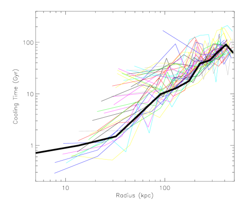
Figure 4: Radial cooling time profiles for each of the 38 BCS clusters in the sample (denoted by the different grey/colour lines, for paper/online publishing respectively). There appears to be a lower bound to the cooling profiles. The thick black line, which traces this lower bound, denotes the average cooling profile for the clusters with a central cooling time less than 2 Gyr.

4.1 Cooling Time Profiles

We have measured the cooling time profiles for all of the clusters in our sample, as shown in Figure 4. While the cooling times in the central bin differ by a few orders in magnitude, we note that there appears to be a prominent, apparently universal lower bound to all of the cooling profiles. The average cooling time profile for the 13 clusters with a central cooling time less than 2 Gyr (thick black line) indicates that there is little difference in the lower bounds for a set of clusters with widely ranging physical characteristics (i.e., temperatures, densities, entropies). While we might expect some sort of boundary given the general nature of how gas cools in clusters, it is physically unclear why a universal boundary that takes the form $t_{c}\propto r^{1.3-1.5}$ (depending on whether one imposes an inner cutoff) would exist. Similarly, Voigt & Fabian (2004) find a very small dispersion in cooling time profiles among their sample of 16 clusters with strong cool cores, with $t_{c}\propto r^{1.3}$.

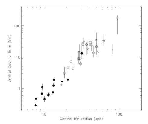
Figure 5: Plot of the central cooling time for the inner radial bin for the 38 BCS clusters in the sample. Filled black, empty, and filled grey symbols denote clusters with detected, undetected, and unobserved H$\alpha$ line emission, respectively (Crawford et al., 1999). Circles denote morphologically regular clusters, while triangles denote double-peaked or disturbed clusters. There is a strong correspondence between low cooling time and detection of H$\alpha$ line emission. The one exception is A2294.

The cooling times for the innermost radial bin are shown in Figure 5 for each cluster. Unfortunately in physical units, the innermost radial bin is both a function of the cluster distance and the overall signal-to-noise of the observation (which in turn depends on whether a cluster exhibits a cool core); hence the apparent correlation in Figure 5. Importantly, the spatial resolution of Chandra is a factor of several smaller than the typical innermost radius adopted (i.e., 0$\aas@@fstack{\prime\prime}$5 corresponds to 1–3 kpc), so any failure to detect a significant cool core in the BCS sample is not due to any limitation on spatial resolution. Also note that because we use the cluster centroid rather than the surface brightness peak, the cooling times inside a few tens of kpc could be biased upward by at most a factor of $\sim$2–3. Alternatively, the central cooling times should be considered upper limits because the strength of cooling depends strongly on the radius at which it is measured, and thus on the signal-to-noise of the observation.

From our determination of cooling times for the innermost radial bin, we find that at least 20 of 38 (53 per cent) BCS clusters in the Chandra sample have central cooling times $<10$ Gyr (mild cool cores) and at least 13 of 38 (34 per cent) have $<2$ Gyr (strong cool cores). To test for any evolution, we compare the cumulative cooling time fractions from the BCS sample to those found for the nearby B55 sample of Peres et al. (1998), who provide cooling times for both the innermost radial bin and 180 kpc (originally 250 kpc in their cosmology). At first glance, the fraction of cool core clusters in our sample as measured from the innermost radial bin would appear to be markedly different from those in the B55 sample (see left plot in Figure 6), implying substantial evolution in the cores of X-ray bright clusters out to $z\sim 0.4$. However, we must exercise caution here, since a direct comparison between the two samples in this manner is problematic. Importantly, the innermost radial bins span a large range in both samples and are significantly smaller in the B55; thus comparing these quantities is not likely to provide a useful yardstick for cooling. Additionally, we note that Peres et al. (1998) measured their cooling times using the surface brightness peak rather than the centroid, so there may be a slight systematic difference between the calculated cooling times for a small fraction of clusters. A final consideration is that the ROSAT observations of the fainter or more distant clusters in the B55 sample may fail to adequately resolve potential cool cores due to limited spatial resolution.

Given the above problems, we instead choose to compare cooling times for the two samples at a fixed intrinsic radius where cooling is still important. Since a large fraction of both samples have innermost radial bins close to or smaller than 50 kpc, this value seems like a sensible radius to use. At 50 kpc, we find that at least 21 of 38 (55 per cent) BCS clusters in the Chandra sample have central cooling times $<10$ Gyr (mild cool cores) and at least 8 of 38 (21 per cent) have $<2$ Gyr (strong cool cores). Because the B55 sample lacks published cooling time profiles, we must interpolate cooling times at 50 kpc. For this purpose, we adopt as an interpolation template the average cooling profile found in Figure 4 for clusters with $t_{c}<2$ Gyr. Comparisons at 50 kpc (middle), as well as at 180 kpc (right), are shown in Figure 6. The apparent differences in the cooling time fractions measured using the innermost radial bin have now all but vanished, demonstrating that there is no detectable evolution in the cool core fraction of clusters out to $z\sim 0.4$. Note that the small discrepancies for short cooling times may be due to our assumed interpolation template. Also note that the fraction of cool cores in either sample has no obvious X-ray luminosity dependence.

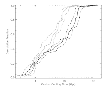
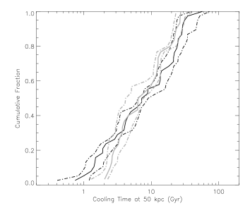
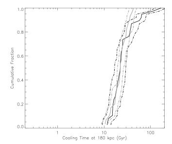
Figure 6: Comparison of the cumulative fraction of cooling times (left: central bin; middle: at 50 kpc; right: at 180 kpc) for the 38 BCS clusters in the sample (black) and the B55 sample of Peres et al. (grey; 1998). The dash-dotted lines denote the 1 $\sigma$ error bars. The large apparent difference seen in the cumulative fraction measured for the central bin disappears when comparisons are made at fixed intrinsic radii.

Let us consider the evolution of a cluster core hosting a cooling flow. First assume that it is isolated with no heating, so that radiative cooling proceeds to drop the gas temperature. Approximating the situation locally as a constant pressure flow, then the cooling time at 50 kpc will decrease by approximately the mean time difference between the samples. The mean redshift of the B55 sample is 0.056 and of the 38 BCS clusters is 0.22, so this difference in our adopted cosmology is about 1.8 Gyr. It is clear from Fig. 6 that this is not occurring since at the 50 per cent level the curves are consistent with each other. Second, we consider the effect of the continual accretion of subclusters by a cluster (e.g., Rowley, Thomas, & Kay, 2004), so that the cool central region undergo adiabatic compression which, for bremsstrahlung cooling appropriate here, varies as $T^{-1}$. This again reduces as time proceeds. Weak to moderate shocks also reduce the cooling time. What is needed is a non-gravitational heat source which offsets the effects of radiative cooling. The similarity between the cumulative curves at 50 kpc for the B55 and BCS samples demonstrates that the heating invoked to balance radiative cooling required to explain the detailed temperature profiles of the clusters must have been in place before the redshift of the BCS. More distant samples are required to determine just when the heating/cooling balance was established.

4.2 Ubiquity of a Cooling “Floor”

As noted in $\S$ 1, the central temperatures in clusters are found to generally drop by less than a factor of $\sim$3–4 with very little cooler gas (e.g., Peterson et al., 2001; Tamura et al., 2001; Peterson et al., 2003; Kaastra et al., 2004). This cooling “floor” is thought to be due to some form of heating (e.g., from an active galactic nucleus, conduction). Figure 7 compares the temperature drop — taken to be ratio between the central bin temperature and the average temperature outside of 180 kpc — to both the 0.5 Mpc power ratios and central cooling times (right) for the 38 BCS clusters in the sample. A similar cooling floor (i.e., a temperature drop of no more than $\approx 3$–4) exists for our cluster sample, and does not appear to correlate with either the strength of the cool core or its general morphology. Interestingly, three of the four lowest temperature drop clusters are merging clusters; inspection of the temperature maps for these clusters indicates that their large temperature ratios are in part likely due to shocks in the outer regions of those clusters. In general, we find that the disturbed clusters in our sample, which all have high $P_{3}/P_{0}$ values, span the entire range of observed temperature ratios, presumably due to the varied merger histories and ages of these clusters.

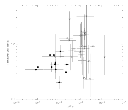
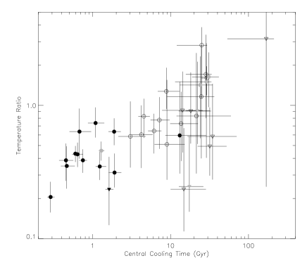
Figure 7: Plot of the ratio between the central bin temperature and the average temperature outside of 180 kpc versus 0.5 Mpc power ratios (left) and central cooling times (right) for the 38 BCS clusters in the sample. Left: Filled black, grey, and empty symbols denote clusters with strong cool cores ($t_{c}<2$ Gyr), weak cool cores ($t_{c}=2$–10 Gyr), and no obvious cool cores ($t_{c}>10$ Gyr), respectively. Right: Filled black, empty, and filled grey symbols denote clusters with detected, undetected, and unobserved H$\alpha$ line emission, respectively (Crawford et al., 1999). Circles denote morphologically regular clusters, while triangles denote double-peaked or disturbed clusters.

4.3 Cooling Time vs. H$\alpha$

A significant fraction of clusters with cool cores have also been shown to exhibit signs of filamentary H$\alpha$ line emission. Since nearly all of the clusters in our sample have H$\alpha$ observations (Crawford et al., 1999), we can examine how useful H$\alpha$ emission is as an indicator of cool cores and cluster morphological properties. Figure 5 demonstrates that 13 of the 38 clusters in the sample show evidence for H$\alpha$ line emission and all but one of these are among the clusters with the very shortest central cooling times. This result strengthens the correlation found by Peres et al. (1998) for relatively nearby clusters. Interestingly, there are another three clusters among the 18 not observed by Chandra that also show evidence for H$\alpha$ line emission. If the H$\alpha$-detected fraction traces the overall cluster population, this would suggest that $\sim$15–20 per cent of the unobserved sources are likely to have strong cool cores and that we might expect a similar overall cool core distribution (i.e., both strong and moderate) among the unobserved clusters as found for the sample sources.

The observed H$\alpha$ and star formation rates requires the mass of H$\alpha$-emitting gas typically to be only a few to a few tens of $M_{\odot}$ yr^-1, whereas classical cooling flows in the observed clusters would require many hundreds of $M_{\odot}$ yr^-1. Thus the presence of H$\alpha$ could imply continuous cooling below the “floor” at a rate of up to a few tens of $M_{\odot}$ yr^-1. Or alternatively, it could imply the presence of conditions necessary for long-lived H$\alpha$.

4.4 Comparison to Power Ratios

A large number of higher redshift clusters have now been found. As these sources are less likely to have the signal-to-noise or spatial resolution to unequivocally detect any potential cool cores, it is instructive to compare our cool core estimates and H$\alpha$ detections for the BCS clusters with their power ratios (which can be measured more reliably under the above conditions). Indeed, Figure 3 demonstrates that the power ratios provide a quantitive assessment of basic morphological trends and can be used as a proxy for central cooling times. Figure 8 bears out this relationship better, showing the strongest correlation between $P_{3}/P_{0}$ versus $t_{\rm cool}$. As expected (e.g., Buote & Tsai, 1996), the more symmetric, compact clusters generally have stronger cool cores and a higher likelihood of H$\alpha$ line detections.

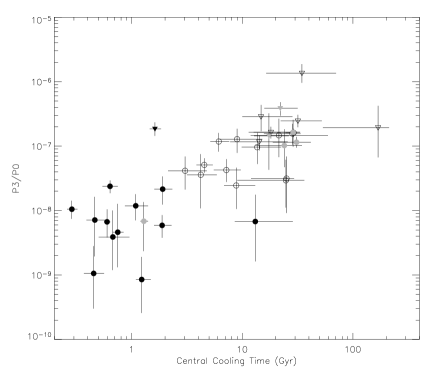
Figure 8: Plot of the $P_{3}/P_{0}$ power ratios and central cooling times for the 38 BCS clusters in the sample. Filled black, empty, and filled grey symbols denote clusters with detected, undetected, and unobserved H$\alpha$ line emission, respectively (Crawford et al., 1999). Circles denote morphologically regular clusters, while triangles denote double-peaked or disturbed clusters.

5 Conclusions

Using a sample of 38 luminous BCS clusters at $z=0.15$–0.4, we find that cool cores still appear to be common at moderate redshift. At 50 kpc, at least 55 per cent of the clusters in our sample possess mild cool cores ($t_{\rm cool}<10$ Gyr) and within the central bin at least 34 per cent possess strong cool cores ($t_{\rm cool}<2$ Gyr). We find that a cooling floor exists for our moderate redshift sample, similar to that found for many nearby clusters, such that the ratio of central to outer temperatures rarely increases above a factor of $\approx$ 3–4. Moreover, comparing the central cooling times to catalogues of central H$\alpha$ emission in BCS clusters, we find a strong correspondence between the detection of H$\alpha$ and short central cooling times. We also find a correlation between the central cooling time and cluster power ratios, indicating that crude morphological measures are a proxy for more rigorous analysis in the face of limited signal-to-noise data.

Comparing our moderate redshift BCS sample to the local B55 sample ($z<0.15$), we find no evidence for any significant evolution in the cumulative cooling time fractions at both 50 kpc and 180 kpc. This suggests that cool cores are already well-developed even at moderate redshifts and, as a consequence, are quite likely to be robust against a wide variety of merger scenarios. It also implies that any additional cooling our sample of clusters underwent over the last $\sim$2–3 Gyr must be balanced by some form of heating. Thus, balanced heating and cooling mechanisms are likely to have already stabilised or been frozen in by this epoch.

Looking toward the future, it will be instructive to analyse Chandra and XMM-Newton observations for a sample of local clusters (such as the B55 sample) in a manner similar to that done here for the BCS sample, so we can perform a more complete and rigorous comparison of the two samples. Further work is also needed to understand when the onset of cool cores occurs. The high fraction of cooling core clusters observed here needs to be tied to the relative dearth of such clusters at the highest redshifts ($z\sim 1$). Another issue is to determine when and how the heating process, which leads to the nearly ubiquitous temperature plateau of a factor of 3–4, occurs. This heating process appears to already be in place for the clusters in our sample, so again we must look to higher redshift samples for clues.

6 Acknowledgements

FEB and RMJ acknowledge support from PPARC. ACF and SWA thank the Royal Society for support.

References

- Allen & Fabian (1997) Allen, S. W. & Fabian, A. C. 1997, MNRAS, 286, 583
- Allen et al. (2001) Allen, S. W., Fabian, A. C., Johnstone, R. M., Arnaud, K. A., & Nulsen, P. E. J. 2001, MNRAS, 322, 589
- Buote & Tsai (1996) Buote, D. A. & Tsai, J. C. 1996, ApJ, 458, 27
- Crawford et al. (1999) Crawford, C. S., Allen, S. W., Ebeling, H., Edge, A. C., & Fabian, A. C. 1999, MNRAS, 306, 857
- Ebeling et al. (1998) Ebeling, H., Edge, A. C., Bohringer, H., Allen, S. W., Crawford, C. S., Fabian, A. C., Voges, W., & Huchra, J. P. 1998, MNRAS, 301, 881
- Ebeling et al. (2000) Ebeling, H., Edge, A. C., Allen, S. W., Crawford, C. S., Fabian, A. C., & Huchra, J. P. 2000, MNRAS, 318, 333
- Edge, Stewart, & Fabian (1992) Edge, A. C., Stewart, G. C., & Fabian, A. C. 1992, MNRAS, 258, 177
- Fabian (1994) Fabian, A. C. 1994, ARA&A, 32, 277
- Gómez, Loken, Roettiger, & Burns (2002) Gómez, P. L., Loken, C., Roettiger, K., & Burns, J. O. 2002, ApJ, 569, 122
- Jerius et al. (2000) Jerius, D., Donnelly, R. H., Tibbetts, M. S., Edgar, R. J., Gaetz, T. J., Schwartz, D. A., Van Speybroeck, L. P., & Zhao, P. 2000, Proc. SPIE Vol. 4012, 17
- Kaastra et al. (2004) Kaastra, J. S., et al. 2004, A&A, 413, 415
- Lupton et al. (2004) Lupton, R., Blanton, M. R., Fekete, G., Hogg, D. W., O’Mullane, W., Szalay, A., & Wherry, N. 2004, PASP, 116, 133
- McGlynn & Fabian (1984) McGlynn, T. A. & Fabian, A. C. 1984, MNRAS, 208, 709
- Peres et al. (1998) Peres, C. B., Fabian, A. C., Edge, A. C., Allen, S. W., Johnstone, R. M., & White, D. A. 1998, MNRAS, 298, 416
- Peterson et al. (2001) Peterson, J. R., et al. 2001, A&A, 365, L104
- Peterson et al. (2003) Peterson, J. R., Kahn, S. M., Paerels, F. B. S., Kaastra, J. S., Tamura, T., Bleeker, J. A. M., Ferrigno, C., & Jernigan, J. G. 2003, ApJ, 590, 207
- Ritchie & Thomas (2002) Ritchie, B. W. & Thomas, P. A. 2002, MNRAS, 329, 675
- Rowley, Thomas, & Kay (2004) Rowley, D. R., Thomas, P. A., & Kay, S. T. 2004, MNRAS, 352, 508
- Sanders et al. (2005) Sanders, J. S., Fabian, A. C., & Taylor, G. B. 2005, MNRAS, 356, 1022
- Tamura et al. (2001) Tamura, T., et al. 2001, A&A, 365, L87
- Townsley et al. (2002) Townsley, L. K., Broos, P. S., Nousek, J. A., & Garmire, G. P. 2002, Nuclear Instruments and Methods in Physics Research A, 486, 751
- Voigt & Fabian (2004) Voigt, L. M. & Fabian, A. C. 2004, MNRAS, 347, 1130