Exploring Cosmological Expansion Parametrizations with the Gold SnIa Dataset
Abstract
We use the SnIa Gold dataset to compare LCDM with 10 representative parametrizations of the recent Hubble expansion history . For the comparison we use two statistical tests; the usual and a statistic we call the p-test which depends on both the value of and the number of the parametrization parameters. The p-test measures the confidence level to which the parameter values corresponding to LCDM are excluded from the viewpoint of the parametrization tested. For example, for a linear equation of state parametrization the LCDM parameter values (, ) are excluded at 75% confidence level. We use a flat prior and . All parametrizations tested are consistent with the Gold dataset at their best fit. According to both statistical tests, the worst fits among the 10 parametrizations, correspond to the Chaplygin gas, the brane world and the Cardassian parametrizations. The best fit is achieved by oscillating parametrizations which can exclude the parameter values corresponding to LCDM at 85% confidence level. Even though this level of significance does not provide a statistically significant exclusion of LCDM (it is less than ) and does not by itself constitute conclusive evidence for oscillations in the cosmological expansion, when combined with similar independent recent evidence for oscillations coming from the CMB and matter power spectra it becomes an issue worth of further investigation.
I Introduction
Converging observational evidence that appeared during the past decade has indicated that we live in a spatially flat universe with low matter density that is currently undergoing accelerated cosmic expansion Riess:2004nr ; Spergel:2003cb ; Readhead:2004gy ; Goldstein:2002gf ; Rebolo:2004vp ; Tegmark:2003ud ; Hawkins:2002sg . This accelerating expansion has been attributed to a dark energy Sahni:2004ai component with negative pressure which can induce repulsive gravity and thus cause accelerated expansion.
The simplest and most obvious candidate for this dark energy is the cosmological constant Sahni:1999gb with equation of state . Such a model predicts an expansion history of the universe which is described by an expansion rate as a function of the redshift given by
| (1) |
where flatness has been imposed and is the single free parameter of this simplest data consistent parametrization (LCDM).
The most sensitive observational probe for testing this type of parametrizations comes from distant standard candles like type Ia supernovae (SnIa). These make it possible to start seeing the varied effects of the universe’s expansion history. The most updated and reliable compilation of SnIa is the Gold dataset recently relased by Riess et al. Riess:2004nr . The authors have compiled a catalog containing 157 SnIa with in the range and visual absorption . The distance modulus of each object has been evaluated by using a set of calibrated methods so that the sample is homogenous in the sense that all the SNeIa have been re-analyzed using the same technique. Thus the resulting Hubble diagram is indeed reliable and accurate. Even though LCDM provides the simplest parametrization consistent with the Gold dataset it has two disadvantages which motivate the search for other models:
-
•
It requires extreme fine tuning of the value of the cosmological constant (coincidence problem).
-
•
It does not provide the best possible fit to the Gold dataset.
In an effort to address these disadvantages three approaches have been followed
-
•
Assume the existence of a homogeneous time dependent scalar field whose dynamics is determined by a specially designed potential so that its energy comes to dominate at present and its negative pressure plays the role of dark energy. Such fields could either have if the sign of the kinetic term is positive (quintessence quintess ) or if the sign of the kinetic term is negative (phantom fields phantom ).
-
•
Consider extensions of general relativity modgrav ; boisseau ; Perivolaropoulos:2003we ; Perivolaropoulos:2002pn ; Alam:2002dv (motivated eg by extra dimensions) which can lead to an accelerating expansion without any modification of the energy momentum tensor.
-
•
Examine arbitrary parametrizations phant-obs2 ; Nesseris:2004wj of the expansion history and focus on maximizing the quality of fit to the Gold dataset.
The problem with the first two approaches which exhibit some physical motivation is that despite their increased number of parameters they very rarely exceed the quality of fit of LCDM. This is not the case for the third approach. Parametrizations which are not constrained to emerge from currently known physical theories provide significantly better fits to the Gold dataset than LCDM. For example it is very hard Vikman:2004dc to construct a physically motivated model predicting an evolution of the dark energy equation of state that crosses the line (phantom divide line). Yet the fit to the Gold dataset improves significantly if such crossing is allowed. The origin of this problem could either be statistical or physical. In the former case we are dealing with a statistical fluctuation of the data and upcoming more detailed datasets will become more consistent with some of the current theories (either minimally coupled scalar fields or modified gravity). In the later case however, if eg the crossing is verified by more detailed data, new theories will have to be constructed. Theoretical attempts in that direction have already started developing using either less physically motivated approaches involving combinations of scalar fields with positive and negative kinetic terms Wei:2005nw ; Hu:2004kh or reconstruction of scalar tensor theories of gravity boisseau ; Perivolaropoulos:2005yv .
In an effort to forecast and support this development it is important to extract the maximal information from the Gold dataset. In particular we wish to address the following question: ‘Given the number of parameters what is an arbitrary (flat and low matter density) parametrization that provides the best fit to the Gold dataset?’ Previous studies attempting to address this type of questions Nesseris:2004wj ; phant-obs2 have either been based Nesseris:2004wj on earlier less reliable datasets Tonry:2003zg ; Barris:2003dq or have not been as extensive in the search of parametrization space phant-obs2 . Here we show that a careful and extensive search of parametrization space can reveal interesting new features of the expansion history hidden in the Gold dataset.
We continue and extend previous work by two of us Nesseris:2004wj and evaluate the quality of fit to the Gold dataset for 10 representative parametrizations of . They include physically motivated parametrizations like brane world Alam:2002dv , Chaplygin gas (first considered in Kamenshchik:2001cp , see also Chimento:2003ta ; Fabris:2001tm ) and Cardassian cosmology, Freese:2005ff as well as arbitrary parametrizations like a linear fit to the equation of state ().
The parametrizations compared have a different number of parameters and therefore their comparison on the basis of how low a they achieve would be biased towards parametrizations with larger number of parameters. The reduced ( per degree of freedom) is an improved statistic in that it has some weak dependence on the number of parameters. We propose however an alternative statistic, we call ‘p-test’ which avoids the above bias and is more appropriate for the comparison of parametrizations with different number of parameters. This statistic along with the general method used for evaluating the quality of fit to the Gold dataset of the parametrizations considered is described in the next section. In section III we present our results for the best fits and discuss their implications and common features.
II Fitting Parametrizations to the Gold dataset
Given a parametrization depending on parameters we can obtain the corresponding Hubble free luminosity distance
| (2) |
Using the maximum likelihood technique press92 we can find the goodness of fit to the corresponding observed coming from the SnIa of the Gold dataset Riess:2004nr . The observational data of the gold dataset are presented as the apparent magnitudes of the SnIa with the corresponding redshifts and errors . The apparent magnitude is connected to as
| (3) |
where is the magnitude zero point offset and depends on the absolute magnitude and on the present Hubble parameter as
| (4) |
The goodness of fit corresponding to any set of parameters is determined by the probability distribution of i.e.
| (5) |
where
| (6) |
and is a normalization factor. If prior information is known on some of the parameters then we can either fix the known parameters using the prior information or ‘marginalize’, i.e. average the probability distribution (5) around the known value of the parameters with an appropriate ‘prior’ probability distribution. The parameters that minimize the expression (6) are the most probable parameter values (the ’best fit’) and the corresponding gives an indication of the quality of fit for the given parametrization: the smaller is, the better the parametrization.
The minimization with respect to the parameter can be made trivially by expanding sfay the of equation (6) with respect to as
| (7) |
where
| (8) |
Equation (7) has a minimum for at
| (9) |
Thus instead of minimizing we can minimize which is independent of . Obviously . Alternatively we could have marginalized over the nuisance parameter thus obtaining Nesseris:2004wj ; Perivolaropoulos:2004yr ; DiPietro:2002cz
| (10) |
to be minimized with respect to . In our analysis we consider the of equation (9) which is already minimized with respect to . In what follows we omit the symbol tilde () for simplicity.
Clearly the value of depends on the parametrization used, and it can decrease arbitrarily close to 0 for large enough number of parameters . Therefore, the value of by itself is not a particularly useful measure of the quality of a given parametrization. It is biased toward parametrizations with larger number of parameters and is therefore useful only in comparing parametrizations with the same number of parameters . Notice however that the reduced ( per degree of freedom) has some weak dependence on the number of parameters and can be an alternative when comparing the quality of fit of parametrizations with different number of parameters.
How can we compare parametrizations with different number of parameters in a more efficient way? This can be achieved by the following procedure: Consider two parametrizations of the expansion history with different number of parameters and and assume that for the parameter values and both parametrizations reduce to a common form eg LCDM i.e.
| (11) | |||||
Let also and be the minimum values of for each parametrization and the value of corresponding to LCDM. Since has a single parameter () which is constrained by prior information (other observations) it is natural to expect that and will be smaller than . Define also , , and . Now and are random variables that obey a probability distribution with and degrees of freedom respectively. Therefore the probability that does not exceed the value is
| (12) | |||||
and similarly for . In eq. (12) is the incomplete function. For and we find corresponding to as expected from well known tables press92 .
Therefore expresses the probability that given the parameter parametrization , the true values of parameters produce a that is less than the value of corresponding to LCDM and therefore LCDM is not realized in nature. In other words it is the confidence level to which LCDM is excluded, from the viewpoint of the parametrization . It is easy to see that increases with but decreases with i.e. a parametrization with many parameters has more difficulty to exclude LCDM unless it can provide a very low (large ). Thus provides a quantitative measure of the quality of a given parametrization which allows comparison with a different parametrization . We call this measure ‘p-test’ and it will be used in what follows to compare the quality of the parametrizations considered.
Another way of comparison of the cosmological models is by using Bayessian theory. In simple terms this is done by forming the so-called Bayes factorJohn:2002gg , where
| (13) |
and denotes the probability (called likelihood for the model ) to obtain the data D if the model is the true one. Generally, is defined as:
| (14) |
for models with one free parameter and where is the prior probability for the parameter . Also, is the likelihood for the parameter in the model and
| (15) |
In the case that has flat prior probabilities, that is we have no prior information on besides that it lies in some range then and
| (16) |
Of course, all this can be generalized for models having more than one parameters.
The interpretation of the Bayes factor is thatJohn:2002gg when there is evidence against when compared with , but it is only worth a bare mention. When the evidence against is definite but not strong. For the evidence is strong and for it is very strong.
In the next section we will use the Bayes factor to compare various parametrizations to LCDM.
III Results-Discussion
In this section we utilize the p-test to rank 10 representative parametrizations of . The comparison of the parametrizations considered is shown in Table I. This is a representative sample among the many more parametrizations we considered but we do not present here for clarity reasons. The rank in Table I is according to the p-test statistic indicated in the third column. A similar rank is obtained using the which is also sensitive to the number of parameters and shown in the last column of Table I. Notice however that the rank according to (shown on the fourth column of Table I) which is insensitive to the number of parameters is somewhat different.
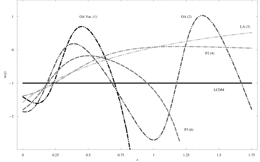
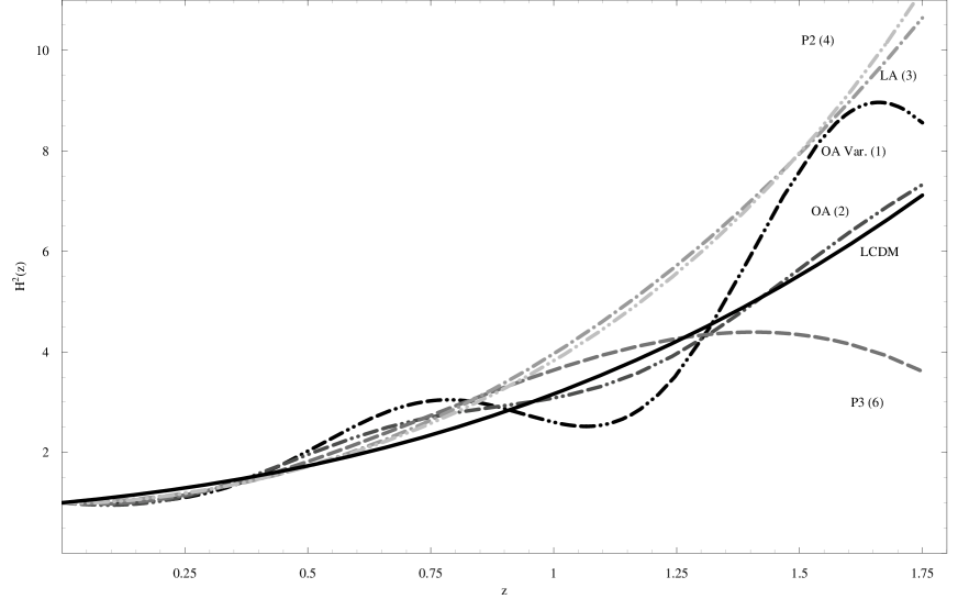
The model name initials of the first column correspond to the following: ‘OA Var (1)’ is an oscillating ansatz with amplitude decreasing with time like . ‘OA (2)’ is a similar ansatz but with constant oscillation amplitude. ‘LA (3)’ is an ansatz used by Linder Linder:2002dt (but proposed earlier in Chevallier:2000qy ) and is derived from an equation of state parameter of the form
| (17) |
interpolating between two constant values of . ‘P2’ is a quadratic polynomial of also discussed in Ref. Alam:2004jy . ‘Linear’ is an ansatz derived by demanding a linear form of the equation of state
| (18) |
‘P3’ is a cubic polynomial of . Here we present the deeper minimum of for P3 which shows oscillating behavior. We have found another minimum less deep which is very similar to the minimum of P2. ‘CA’ is an ansatz based on the generalized cardassian cosmology Freese:2005ff . ‘Quiess’ corresponds to dark energy with constant equation of state . ‘MCG’ is a modified form Chimento:2003ta of the Chaplygin gas Fabris:2001tm . We have tested several variants of this ansatz but they all have a fit that is marginally distinguishable from LCDM. ‘Brane2’ is an ansatz motivated from brane world cosmology Alam:2002dv . It appears in two variants which involve a change of sign in the square root appearing in but we find no significant difference in the quality of fit between the two variants (‘Brane1’ and ‘Brane2’); they are both practically indistinguishable from LCDM.
| Model | , () | p-test | Best fit parameters | ||
|---|---|---|---|---|---|
| OA Var. (1) | 0.85 | 171.733 | 1.115 | ||
| , | |||||
| OA (2) | 0.81 | 172.368 | 1.119 | ||
| LA (3) | 0.79 | 173.928 | 1.122 | ||
| P2 (4) | 0.78 | 174.207 | 1.124 | ||
| Linear (5) | 0.75 | 174.365 | 1.125 | ||
| P3 (6) | 0.74 | 173.155 | 1.124 | ||
| CA (7) | 0.50 | 175.758 | 1.134 | ||
| Quiess (8) | 0.15 | 177.091 | 1.135 | ||
| GCG (9) | 0.031 | 177.064 | 1.142 | ||
| Brane 2 (10) | 0.027 | 177.071 | 1.142 | ||
| LCDM | - | 177.072 | 1.135 |
In all cases we have assumed priors corresponding to flatness and . For a prior we have found no significant changes in the results of Table I. The following are noteworthy features of Table I:
-
•
The ansatz giving the best fit to the Gold dataset is an oscillating parametrization where the amplitude of the oscillations decreases like the third power of the scale factor. This type of decreasing amplitude oscillations can be induced by an oscillating scalar field minimally or non-minimally coupled (e.g. the radion Perivolaropoulos:2003we ; Perivolaropoulos:2002pn ). With respect to this parametrization the simplest data consistent parametrization (LCDM) is excluded at the confidence level. This level of significance is clearly not enough to disfavor LCDM but it may provide a hint for interesting better fits to the data.
-
•
The cubic polynomial parametrization P3 which provides a fairly good fit to the Gold dataset (the third best ) also shows indications of oscillations at its best fit despite the fact that no oscillating functions are built in the parametrization. We have seen a similar behavior in other power law parametrizations even though we have not included those in Table I to avoid confusion.
-
•
Physically motivated parametrizations like the Chaplygin gas, brane-world models and Cardassian cosmology provide marginally better fits than LCDM and are disfavored by our test due to their larger number of parameters compared to LCDM.
-
•
Parametrizations that allow and crossing of the phantom divide line produce significantly better fits to the Gold dataset.
In Table II, we consider the same parametrizations, as in Table I, but now we have marginalized over . We have used uniform marginalization in the range . We also show the Bayes factor for each model against LCDM, calculated with the techniques described in the previous section and assuming uniform probability distribution of the parameters within their range.
Also, as expected, after marginalizing over , the error bars of the best-fit parameters have increased. For example, for the P2 model, in the case of the prior, we found and , but after marginalizing and . In the same fashion, for the LA model we found in the first case and and in the latter and .
In Figs 1 and 2 we show the best fit and for 6 representative parametrizations of Table I.
Our result for the improved fit of oscillating parametrizations is consistent with a previous finding by two of us Nesseris:2004wj using an earlier SnIa dataset Tonry:2003zg ; Barris:2003dq . Clearly, even though LCDM is disfavored at the 85% confidence level with respect to the oscillating parametrization this is not enough to offer conclusive evidence for the existence of oscillations in the cosmological expansion.
| Model | Bayes Factor | |||
|---|---|---|---|---|
| OA Var. (1) | 9.03 | 176.442 | 1.146 | |
| OA (2) | 2.56 | 177.029 | 1.150 | |
| LA (3) | 2.63 | 178.676 | 1.153 | |
| P2 (4) | - | 178.874 | 1.154 | |
| Linear (5) | 2.50 | 179.173 | 1.156 | |
| P3 (6) | 3.68 | 177.859 | 1.155 | |
| CA (7) | 0.78 | 182.308 | 1.176 | |
| Quiess (8) | 0.98 | 181.614 | 1.164 | |
| GCG (9) | 1.26 | 181.394 | 1.177 | |
| Brane 2 (10) | - | 182.326 | 1.176 | |
| LCDM | 1 | 182.326 | 1.161 |
However, it is recently becoming clear that the possibility of cosmological expansion oscillations is favored by a number of independent additional factors, observational and theoretical. The theoretical factors include the following:
-
1.
The eternal acceleration predicted by LCDM and by most other parametrizations creates problems in string theory where asymptotic flatness of space-time is required 1 . Theoretical models (using eg special quintessence potentials or generalizations of the Einstein action and extra dimensions Collins:2001ic ) have been proposed Rubano:2003er to cure this problem by cosmological expansion oscillations. Unfortunately, these modelsRubano:2003er do not predict crossing of the as indicated by the data because they are based on minimally coupled scalar fields.
-
2.
A periodic expansion rate of the universe could resolve the cosmic coincidence problem. In an oscillating expansion setup, the present period of acceleration would be nothing surprising; it would merely be one of the many other accelerating periods that also occurred in the past Dodelson:2001fq ; 2 .
-
3.
Models with extra dimensions require a mechanism to stabilize the size of extra dimensions (the radion field). However, since the radion field also couples to the redshifting matter density (it behaves like a Brans-Dicke scalar) its equilibrium point is slowly shifting with time and radion oscillations are generically excited. The energy density of these oscillations is dropping approximately like the third power of the scale factor Perivolaropoulos:2002pn . It is exactly this power that gives the best fit of the SnIa data! The constraints imposed on such low frequency oscillations by local gravity tests can be relaxed by taking into account the increased average matter density in the neighborhood of the solar system which can significantly increase the local effective mass of the radion Brax:2004ym .
The observational factors favoring oscillating expansion include the following:
-
1.
Superimposed oscillations Martin:2004yi or glitches Hunt:2004vt in the CMB multipole moments can improve the fit to the first year Wilkinson Microwave Anisotropies Probe (WMAP) data. The corresponding drop in the for superposed oscillations was found to be which is statistically significant Martin:2004yi . These oscillations were attributed to new physics taking place at the inflationary phase reflecting on the produced fluctuations power spectrum. However, small amplitude oscillations of the cosmological expansion could also induce similar effects with remnants in the present day expansion rate.
-
2.
The 128 Mpc periodicity in the galaxy redshift distribution was first observed in pencil redshift surveys and confirmed more recently by large scale redshift surveys Bajan:2003yv ; Broadhurst:1990be ; Einasto:1997md ; a8 . This periodic distribution could either be attributed to specific features of the matter spectrum (coming eg from the acoustic oscillations Eisenstein:2005su at recombination or from exotic physics), or to oscillating cosmological expansion a11 ; a13a . Even though the origin of this periodicity remains an unresolved issue it should be pointed out that a recent study has indicated that the probability that such periodicity emerges statistically in a LCDM cosmology is less than 0.1% Gonzalez:2000qy ; Yoshida:2000zq .
In conclusion, we have performed an extensive comparative study in parametrization space and have evaluated the quality of fit of several parametrizations to the Gold dataset. In comparing the quality of fit we have used two statistics: the value of at its minimum () which is independent of the parametrization number of parameters and the p-test () which evaluates the quality of fit with respect to LCDM and depends on both and the number of parametrization parameters . According to both statistics the best fit to the Gold dataset is achieved by an oscillating parametrization with oscillating amplitude decreasing like the inverse cubic power of the scale factor. Even a cubic polynomial parametrization is showing oscillating behavior at best fit. We stress however that the statistical significance of the improved fit of oscillating and other parametrizations we found is at less than level and is therefore not enough to exclude the LCDM parametrization. It does provide however a hint towards parametrizations that are clearly more probable than LCDM to be realized in nature on the basis of the Gold dataset.
We have also briefly reviewed the theoretical and observational evidence that has been accumulating during the recent years in support of such oscillations. The particular type of oscillations that are providing the best fit to the equation of state exhibit crossings of the divide line. These crossings can not be reproduced in any single field quintessence or phantom model and probably require non-minimally coupled theories for their physical interpretation.
The mathematica file with the numerical analysis of the paper can be found at http://leandros.physics.uoi.gr/goldfit.htm
Acknowledgements
The work of S.N. and L.P. was supported by the program PYTHAGORAS-1 of the Operational Program for Education and Initial Vocational Training of the Hellenic Ministry of Education under the Community Support Framework and the European Social Fund. The work of R.L. was supported by the Spanish Ministry of Education and Culture through research grant FIS2004-01626. We would also like to thank S. P. Lee for pointing out some typographic errors on the manuscript.
References
- (1) A. G. Riess et al. [Supernova Search Team Collaboration], Astrophys. J. 607, 665 (2004).
- (2) D. N. Spergel et al. [WMAP Collaboration], Astrophys. J. Suppl. 148, 175 (2003).
- (3) A. C. S. Readhead et al., Astrophys. J. 609, 498 (2004).
- (4) J. H. Goldstein et al., Astrophys. J. 599, 773 (2003) [arXiv:astro-ph/0212517].
- (5) R. Rebolo et al., MNRAS 353 747R (2004), arXiv:astro-ph/0402466.
- (6) M. Tegmark et al. [SDSS Collaboration], Phys. Rev. D 69, 103501 (2004).
- (7) E. Hawkins et al., Mon. Not. Roy. Astron. Soc. 346, 78 (2003).
- (8) V. Sahni, arXiv:astro-ph/0403324; D. Huterer and M. S. Turner, Phys. Rev. D 64, 123527 (2001) [arXiv:astro-ph/0012510]; R. Bean and A. Melchiorri, Phys. Rev. D 65, 041302 (2002) [arXiv:astro-ph/0110472].
- (9) V. Sahni and A. A. Starobinsky, Int. J. Mod. Phys. D 9, 373 (2000) [arXiv:astro-ph/9904398]; S. M. Carroll, Living Rev. Rel. 4, 1 (2001) [arXiv:astro-ph/0004075]; P. J. E. Peebles and B. Ratra, Rev. Mod. Phys. 75, 559 (2003) [arXiv:astro-ph/0207347]; T. Padmanabhan, Phys. Rept. 380, 235 (2003) [arXiv:hep-th/0212290].
- (10) B. Ratra and P.J.E. Peebles, Phys. Rev. D37, 3406 (1988); Rev. Mod. Phys. 75, 559 (2003) [arXiv:astro-ph/0207347]; C. Wetterich, Nucl. Phys. B 302, 668(1988); P.G.Ferreira and M. Joyce, Phys. Rev. D.58,023503(1998); P.Brax and J.Martin, Phys. Rev. D.61,103502(2000); L.A. Urena-Lopez and T. Matos, Phys. Rev. D.62,081302(2000); T.Barreiro, E.J.Copeland and N. J. Nunes, Phys. Rev. D.61,127301 (2000); D.Wands, E. J. Copeland and A. R. Liddle, Phys. Rev. D. 57, 4686 (1998); A. R. Liddle and R. J. Scherrer, Phys. Rev. D 59, 023509 (1998); R. R. Caldwell, R. Dave and P. Steinhardt, Phys. Rev. Lett 80, 1582 (1998); I. Zlatev, L. Wang and P. Steinhardt, Phys. Rev. Lett. 82, 896 (1999); S. Dodelson, M. Kaplinghat and E. Stewart, Phys. Rev. Lett. 85, 5276(2000); V. B. Johri, Phys. Rev. D.63,103504(2001); V. B. Johri, Class. Quant. Grav.19,5959 (2002); V. Sahni and L. Wang, Phys. Rev. D.62, 103517 (2000); M. Axenides and K. Dimopoulos, JCAP 0407, 010 (2004)[arXiv:hep-ph/0401238]; M. Doran and J. Jaeckel Phys. Rev. D 66, 043519 (2002) [arXiv:astro-ph/0203018]; B. A. Bassett, P. S. Corasaniti and M. Kunz,Astrophys. J. 617, L1 (2004) [arXiv:astro-ph/0407364].
- (11) R. R. Caldwell, Phys. Lett. B 545, 23 (2002) [arXiv:astro-ph/9908168]; P. F. Gonzalez-Diaz, Phys. Lett. B 586, 1 (2004) [arXiv:astro-ph/0312579]; P. Singh, M. Sami and N. Dadhich, Phys. Rev. D 68, 023522 (2003) [arXiv:hep-th/0305110]. G. Calcagni, arXiv:gr-qc/0410111; V. B. Johri, Phys. Rev. D 70, 041303 (2004) [arXiv:astro-ph/0311293]; V. K. Onemli and R. P. Woodard, Class. Quant. Grav.19, 4607 (2000); S. Hannestad and E. Mortsell, Phys. Rev. D66,063508(2002); S. M. Carroll, M. Hoffman and M. Trodden, Phys. Rev. D 68, 023509 (2003) [arXiv:astro-ph/0301273]; P. H. Frampton, hep-th/0302007; P. F. Gonzalez-Diaz and C. L. Siguenza, Nucl. Phys. B 697, 363 (2004) [arXiv:astro-ph/0407421]; G.W.Gibbons, hep-th/0302199;B.Mcinnes, astro-ph/0210321; L. P. Chimento and R. Lazkoz, Phys. Rev. Lett. 91, 211301 (2003)[arXiv:gr-qc/0307111]; H. Stefancic,Phys. Lett. B 586, 5 (2004) [arXiv:astro-ph/0310904]; H. Stefancic,Eur. Phys. J. C 36, 523 (2004) [arXiv:astro-ph/0312484]; P. F. Gonzalez-Diaz, Phys. Rev. D 69, 063522 (2004)[arXiv:hep-th/0401082]; V. K. Onemli and R. P. Woodard, Phys. Rev. D 70, 107301 (2004) [arXiv:gr-qc/0406098]; T. Brunier, V. K. Onemli and R. P. Woodard, Class. Quant. Grav. 22, 59 (2005) [arXiv:gr-qc/0408080]; E. Elizalde, S. Nojiri and S. D. Odintsov, Phys. Rev. D 70, 043539 (2004) [arXiv:hep-th/0405034]; S. Nojiri and S. D. Odintsov, Phys. Lett. B 571, 1 (2003) [arXiv:hep-th/0306212]; S. Nojiri and S. D. Odintsov, Phys. Lett. B 562, 147 (2003) [arXiv:hep-th/0303117]; I. Brevik, S. Nojiri, S. D. Odintsov and L. Vanzo, Phys. Rev. D 70, 043520 (2004) [arXiv:hep-th/0401073].
- (12) C. Deffayet, G. Dvali and G. Gabadadze, Phys. Rev. D65, 044023 (2002); J. S. Alcaniz, Phys. Rev. D 65, 123514 (2002). astro-ph/0202492; E. V. Linder, Phys. Rev. Lett. 90, 091301 (2003); L. Perivolaropoulos, Phys. Rev. D 67, 123516 (2003) [arXiv:hep-ph/0301237]; D.F.Torres, Phys. Rev. D66,043522(2002).
- (13) B. Boisseau, G. Esposito-Farese, D. Polarski and A. A. Starobinsky, Phys. Rev. Lett. 85, 2236 (2000)[arXiv:gr-qc/0001066].
- (14) L. Perivolaropoulos, Phys. Rev. D 67, 123516 (2003) [arXiv:hep-ph/0301237].
- (15) L. Perivolaropoulos and C. Sourdis, Phys. Rev. D 66, 084018 (2002) [arXiv:hep-ph/0204155].
- (16) V. Sahni and Y. Shtanov, JCAP 0311, 014 (2003) [arXiv:astro-ph/0202346]; U. Alam and V. Sahni, arXiv:astro-ph/0209443.
- (17) U. Alam, V. Sahni, T. D. Saini and A. A. Starobinsky, Mon. Not. Roy. Astron. Soc. 354, 275 (2004) [arXiv:astro-ph/0311364]; T. R. Choudhury and T. Padmanabhan, Astron. Astrophys. 429, 807 (2005) astro-ph/0311622; Y. Wang and P. Mukherjee, Astrophys. J. 606, 654 (2004) [arXiv:astro-ph/0312192]; D. Huterer and A. Cooray, Phys. Rev. D 71, 023506 (2005); R. A. Daly and S. G. Djorgovski, Astrophys. J. 597, 9 (2003) [arXiv:astro-ph/0305197]; J. S. Alcaniz, Phys. Rev. D69, 083521 (2004) astro-ph/0312424; J. A. S. Lima, J. V. Cunha and J. S. Alcaniz, Phys. Rev. D 68, 023510 (2003) [arXiv:astro-ph/0303388]; A. Upadhye, M. Ishak and P. J. Steinhardt, Phys. Rev. D 72, 063501 (2005), arXiv:astro-ph/0411803; D. A. Dicus and W. W. Repko, Phys. Rev. D 70, 083527 (2004) [arXiv:astro-ph/0407094]; Y. G. Gong, Class. Quant. Grav. 22, 2121 (2005), arXiv:astro-ph/0405446.
- (18) S. Nesseris and L. Perivolaropoulos, Phys. Rev. D 70, 043531 (2004) [arXiv:astro-ph/0401556].
- (19) A. Vikman, Phys. Rev. D 71, 023515 (2005) [arXiv:astro-ph/0407107].
- (20) Z. K. Guo, Y. S. Piao, X. M. Zhang and Y. Z. Zhang, arXiv:astro-ph/0410654; B. Feng, X. L. Wang and X. M. Zhang, Phys. Lett. B 607, 35 (2005) [arXiv:astro-ph/0404224]; B. Feng, M. Li, Y. S. Piao and X. Zhang, arXiv:astro-ph/0407432; X. F. Zhang, H. Li, Y. S. Piao and X. M. Zhang, arXiv:astro-ph/0501652; H. Wei and R. G. Cai, arXiv:hep-th/0501160.
- (21) W. Hu, Phys. Rev. D 71, 047301 (2005) [arXiv:astro-ph/0410680].
- (22) L. Perivolaropoulos, JCAP 10, 001 (2005), arXiv:astro-ph/0504582.
- (23) J. L. Tonry et al., Astrophys. J. 594, 1 (2003) [arXiv:astro-ph/0305008].
- (24) B. J. Barris et al., Astrophys. J. 602, 571 (2004) [arXiv:astro-ph/0310843].
- (25) A. Y. Kamenshchik, U. Moschella and V. Pasquier, Phys. Lett. B 511, 265 (2001) [arXiv:gr-qc/0103004].
- (26) L. P. Chimento, Phys. Rev. D 69 (2004) 123517 [arXiv:astro-ph/0311613].
- (27) J. C. Fabris, S. V. B. Goncalves and P. E. de Souza, Gen. Rel. Grav. 34, 53 (2002) [arXiv:gr-qc/0103083]; N. Bilic, G. B. Tupper and R. D. Viollier, Phys. Lett. B 535, 17 (2002) [arXiv:astro-ph/0111325]; A. Dev, D. Jain and J. S. Alcaniz, Phys. Rev. D 67, 023515 (2003) [arXiv:astro-ph/0209379]; M. Makler, S. Quinet de Oliveira and I. Waga, Phys. Lett. B 555, 1 (2003) [arXiv:astro-ph/0209486]; R. Bean and O. Dore, Phys. Rev. D 68, 023515 (2003) [arXiv:astro-ph/0301308]; L. P. Chimento and R. Lazkoz, Phys. Lett. B 615, 146 (2005), arXiv:astro-ph/0411068; D. J. Liu and X. Z. Li, Chin. Phys. Lett. 22, 1600 (2005), arXiv:astro-ph/0501115.
- (28) K. Freese, New Astron. Rev. 49, 103 (2005), arXiv:astro-ph/0501675; Z. H. Zhu and M. K. Fujimoto, Astrophys. J. 585, 52 (2003) [arXiv:astro-ph/0303021]; J. M. Cline and J. Vinet, Phys. Rev. D 68, 025015 (2003) [arXiv:hep-ph/0211284]; K. Freese, Nucl. Phys. Proc. Suppl. 124, 50 (2003) [arXiv:hep-ph/0208264]; K. Freese and M. Lewis, Phys. Lett. B 540, 1 (2002) [arXiv:astro-ph/0201229].
- (29) W. H. Press et. al., ‘Numerical Recipes’, Cambridge University Press (1994).
- (30) S. Fay, private communication.
- (31) L. Perivolaropoulos, Phys. Rev. D 71, 063503 (2005) [arXiv:astro-ph/0412308].
- (32) E. Di Pietro and J. F. Claeskens, Mon. Not. Roy. Astron. Soc. 341, 1299 (2003) [arXiv:astro-ph/0207332].
- (33) M. V. John and J. V. Narlikar, Phys. Rev. D 65, 043506 (2002) [arXiv:astro-ph/0111122].
- (34) E. V. Linder, Phys. Rev. D 68, 083503 (2003) [arXiv:astro-ph/0212301].
- (35) M. Chevallier and D. Polarski, Int. J. Mod. Phys. D 10, 213 (2001) [arXiv:gr-qc/0009008].
- (36) U. Alam, V. Sahni and A. A. Starobinsky, JCAP 0406, 008 (2004) [arXiv:astro-ph/0403687].
- (37) S. Hellerman, N. Kaloper, and L. Susskind, J. High Energy Phys. 0106, 003 (2001).
- (38) H. Collins and B. Holdom, Phys. Rev. D 65, 124014 (2002) [arXiv:hep-ph/0110322].
- (39) C. Rubano, P. Scudellaro, E. Piedipalumbo and S. Capozziello, Phys. Rev. D 68, 123501 (2003) [arXiv:astro-ph/0311535].
- (40) G. Barenboim, O. Mena and C. Quigg, Phys. Rev. D 71, 063533 (2005) [arXiv:astro-ph/0412010]; G. Barenboim, O. M. Requejo and C. Quigg, arXiv:astro-ph/0510178.
- (41) S. Dodelson, M. Kaplinghat and E. Stewart, Phys. Rev. Lett. 85, 5276 (2000) [arXiv:astro-ph/0002360].
- (42) P. Brax, C. van de Bruck and A. C. Davis, JCAP 0411, 004 (2004) [arXiv:astro-ph/0408464].
- (43) J. Martin and C. Ringeval, JCAP 0501, 007 (2005) [arXiv:hep-ph/0405249]; J. Martin and C. Ringeval, Phys. Rev. D 69, 127303 (2004); J. Martin and C. Ringeval, Phys. Rev. D 69, 083515 (2004) [arXiv:astro-ph/0310382].
- (44) P. Hunt and S. Sarkar, Phys. Rev. D 70, 103518 (2004) [arXiv:astro-ph/0408138].
- (45) K. Bajan, M. Biernacka, P. Flin, W. Godlowski, V. Pervushin and A. Zorin, Spacetime and Substance.4:225-228,2003, arXiv:astro-ph/0408551.
- (46) T. J. Broadhurst, R. S. Ellis, D. C. Koo and A. S. Szalay, Nature 343, 726 (1990).
- (47) J. Einasto et al., Nature 385, 139 (1997). arXiv:astro-ph/9701018.
- (48) R. Kirshner, Nature, 385, 122 (1997).
- (49) D. J. Eisenstein et al., arXiv:astro-ph/0501171.
- (50) M. Morikawa, , ApJ, 362, L37 (1990).
- (51) H. Quevedo, M. Salgado, D. Sudarsky, GRG, 31, 767 (1999).
- (52) J. A. Gonzalez, H. Quevedo, M. Salgado and D. Sudarsky, Astron. Astrophys. 362, 835 (2000) [arXiv:astro-ph/0010437].
- (53) N. Yoshida et al. [The VIRGO Collaboration], Mon. Not. Roy. Astron. Soc. 325, 803 (2001) [arXiv:astro-ph/0011212].